Article

Coordination of Multiple Biomimetic Autonomous Underwater Vehicles Using Strategies Based on the Schooling Behaviour of Fish

by
Jonathan McColgan
* and
Euan W. McGookin
Division of Aerospace Sciences, School of Engineering, University of Glasgow, Glasgow G12 8QQ, UK
*
Author to whom correspondence should be addressed.
Robotics 2016, 5(1), 2; https://doi.org/10.3390/robotics5010002
Submission received: 13 November 2015 / Revised: 21 December 2015 / Accepted: 28 December 2015 / Published: 13 January 2016
(This article belongs to the Special Issue Underwater Robotics)

Abstract

:
Biomimetic Autonomous Underwater Vehicles (BAUVs) are Autonomous Underwater Vehicles (AUVs) that employ similar propulsion and steering principles as real fish. While the real life applicability of these vehicles has yet to be fully investigated, laboratory investigations have demonstrated that at low speeds, the propulsive mechanism of these vehicles is more efficient when compared with propeller based AUVs. Furthermore, these vehicles have also demonstrated superior manoeuvrability characteristics when compared with conventional AUVs and Underwater Glider Systems (UGSs). Further performance benefits can be achieved through coordination of multiple BAUVs swimming in formation. In this study, the coordination strategy is based on the schooling behaviour of fish, which is a decentralized approach that allows multiple AUVs to be self-organizing. Such a strategy can be effectively utilized for large spatiotemporal data collection for oceanic monitoring and surveillance purposes. A validated mathematical model of the BAUV developed at the University of Glasgow, RoboSalmon, is used to represent the agents within a school formation. The performance of the coordination algorithm is assessed through simulation where system identification techniques are employed to improve simulation run time while ensuring accuracy is maintained. The simulation results demonstrate the effectiveness of implementing coordination algorithms based on the behavioural mechanisms of fish to allow a group of BAUVs to be considered self-organizing.

1. Introduction

Approximately 71% of the Earth’s surface is comprised of water [1], yet it is estimated that as much as 95% of this vast resource remains unexplored to a similar resolution that is available for the surface of the moon [2]. Although essential to all known life, the salt water medium which makes up the Earth’s oceans, and affects global climate and weather patterns also provides a hostile environment for exploration [3]. In particular, the oceans present a hazardous environment for the safe and successful operation of a group of underwater vehicles known as Autonomous Underwater Vehicles (AUVs). Unlike other autonomous platforms (e.g., Unmanned Aerial Vehicles (UAVs) and Unmanned Surface Vehicles (USVs)), AUVs are operated in an environment where access to accurate positional data and a reliable communication medium is severely limited. Nonetheless, AUVs have evolved from research platforms used exclusively by academic institutions in the 1950s through to the present day where these highly autonomous systems are used within the oil and gas industry for pipeline inspection [4] as well as being utilized for search and recovery missions [5], maritime surveillance [6], and sampling previously unexplored regions of the Earth such as under the Arctic ice pack [7].
However, as a result of AUVs being untethered, the power available to these vehicles is finite and as such, their range and endurance is limited [8]. While it is now common for AUV mission endurance to be measured in days, the operation of a single vehicle for large spatiotemporal data collection operations, such as oil plume tracking [9], is inadequate. Therefore, the only way to satisfy this requirement is to operate a groups of AUVs within a multi-vehicle deployment which has been proven to improve the efficiency of current missions as described in [10,11].
Despite the improved efficiencies offered by multi-vehicle coordination, the difficulties associated with the underwater environment present a number of substantial technological barriers which must be overcome before fully autonomous multi-vehicle coordination is realized. At present, the greatest of these challenges is establishing a suitable communication strategy among the vehicles which is tolerant to the limitations of the underwater acoustic communication channel [3,12]. Nevertheless, a number of sea-trials have been completed since the start of the 21st century that have demonstrated not only the feasibility of operating multiple AUVs within a group structure but also the advantages of doing so [10,11].
While the trials discussed above are essential to the realization of a self-coordinating group of AUVs, the costs associated with completing such trials do not present an economically viable method to develop, test and analyse the various potential coordination algorithms associated with the deployment of a group of AUVs. Instead, extensive testing and optimization of the algorithms can be completed in a more time efficient manner using mathematical modelling and simulation techniques [13].
Mathematical modelling involves representing the dynamics and kinematics of a vehicle through a serious of differential equations that when integrated, simulate the motion of that particular vehicle. When used correctly, mathematical modelling provides a powerful tool through all phases of the design process. Therefore, this paper uses mathematical modelling techniques to accurately represent the dynamics of a particular type of AUV known as RoboSalmon, which has been designed, built and tested at the University of Glasgow [14].
RoboSalmon is classed as a Biomimetic Autonomous Underwater Vehicle (BAUV). These vehicles adopt the same propulsion and steering mechanisms as real fish [14,15,16,17,18] and in doing so, their propulsive mechanism has been found to be more efficient at low speeds when compared with traditional propeller based AUVs [19] but also poses far greater manoeuvrability characteristics [20]. As a result, BAUVs are more suited to operating in confined environments and therefore make an ideal candidate vehicle for assessing the feasibility of coordinating multiple vehicles in close proximity to one another.
However, in order for a group of vehicles to complete the large scale spatiotemporal data collection missions discussed above, it is apparent that the vehicles must be able to coordinate themselves to ensure the given survey area is mapped efficiently. To achieve this, the coordination algorithms must ensure that all vehicles within the group are spaced appropriately, move with a common heading angle while avoiding collisions between neighbouring vehicles.
One particular coordination strategy that satisfies the above criteria is related to the behavioural mechanism utilized by fish within large school structures. This mechanism enforces a number of behavioural zones around each fish, which, depending on the distance to its nearest neighbours, results in the fish manoeuvring in an attractive, orientating or repulsive manner [21,22,23].
Therefore, it is the aim of this paper to demonstrate that coordination algorithms based on the behavioural mechanisms of fish provides a suitable and easily adaptive method to allow a group BAUVs to be considered self-coordinating. Furthermore, the work presented in this paper shows the benefits of employing reduced fidelity versions of the current validated mathematical model of RoboSalmon for multi-vehicle coordination studies [20].
This study is presented in this paper in the following manner. Section 2 briefly describes the RoboSalmon vehicle and compares it with the other types of Unmanned Underwater Vehicles. It then discusses in detail the current mathematical model of RoboSalmon, its run time performance and methodologies implemented to improve its run time. Results from the validation process are presented in order to ensure that the reduced fidelity models still accurately represent the dynamics of the RoboSalmon vehicle. Section 3 will describe the implementation of the coordination algorithms discussed above with the inclusion of realistic communication constraints. Section 4 presents the results from the simulations involving the coordination algorithms and finally, Section 5 presents the conclusions of the work completed in this paper.

2. RoboSalmon—Biomimetic Autonomous Underwater Vehicle (BAUV)

2.1. Vehicle Design

The design of the RoboSalmon vehicle is based on the North Atlantic Salmon (see Figure 1a). This particular species of fish is considered to be of subcarangiform which means that 50%–60% of its body is used to generate the propulsive wave required to generate the body’s motion [16]. Therefore, in order to mimic this particular type of locomotion, the RoboSalmon vehicle (Figure 1b) is composed of two sections: a forward rigid body section and a fully actuated segmented tail section, which allows the swimming gait of the North Atlantic Salmon to be replicated.
Figure 1. RoboSalmon BAUV designed and built at the University of Glasgow [20]: (a) RoboSalmon vehicle; and (b) Schematic diagram. Reproduced with permission from Naddi Mazlan, PhD Thesis [20].
Robotics 05 00002 g001
In order to assess RoboSalmon’s performance against that of other Unmanned Underwater Vehicles (UUVs), a number of performance parameters are presented in Table 1 for comparison purposes. The data contained within Table 1 can be obtained from [20,24,25,26,27,28].
Table 1. Typical performance parameters for the various classes of UUVs.
Class of AUVVehicle NameVehicle Length (m)Surge Velocity (m/s)Turning Radius (m)
AUVIver2-5801.62.064
Bluefin-9M2.52.572.63
UGSSLOCUM1.520.27
Spray20.2630
BAUVRoboSalmon0.90.140.6
BioSwimmer1.522.571
As presented in Table 1, for vehicles of similar length the manoeuvrability characteristics of BAUVs are superior to those achievable using AUVs and UGS which would suggest that these vehicles are particularly suited to operating within confined environments [29]. The following section describes in detail the current validated mathematical model of the RoboSalmon vehicle.

2.2. Mathematical Model

As shown in Figure 2, the mathematical model of RoboSalmon can be separated into three subsystems: Tail Actuator Dynamics, Vehicle Dynamics and finally, the vehicle’s Guidance System.
Figure 2. Mathematical model structure.
Robotics 05 00002 g002
The values within each subsystem of Figure 2 demonstrate the various rates at which functionality is evaluated within the model, ranging from 1000 Hz down to a single hertz. As a result, the mathematical model is able to evaluate the fast dynamics with smaller time constants while the slower dynamic sections are evaluated with larger time constants. This methodology, known as multi-rate simulation, improves the computational efficiency of the model without sacrificing numerical accuracy. Finally, each of the subsystem presented in Figure 2 are described in more detail in the following sections.

2.2.1. Tail Actuator Dynamics

As mentioned previously, the purpose of the fully actuated tail section of the vehicle is to replicate the swimming gait of the Atlantic salmon. It achieves this through the combined motion of ten, individually controlled revolute joints attached to a replica caudal fin. The structure of the system used to control this motion of each motor within the mathematical model is presented below in Figure 3.
Figure 3. Structure of tail actuator system within mathematical model.
Robotics 05 00002 g003
Figure 3 demonstrates that the input for each motor, j, is a user defined step angle. These angles are defined in terms of replicating the swimming gait of the actual fish [14]. They are chosen such that the resultant motion of the tail is an approximation of the travelling wave equation which Lighthill suggested replicates the undulatory nature of fish locomotion [30].
As shown in Figure 3, for each motor, i, the defined step angles are compared with the motor’s present angular position to produce an error angle, Δ θ j which is the input to the control system. The control system is a standard PID controller which can be represented by the following equation:
V j = K p Δ θ j + K i Δ θ j d t +   K d d Δ θ j d t
where Δ θ represents the aforementioned comparison error between the required and demanded motor angle and V j represents the required voltage from each motor to achieve the desired step angle. K p ,   K i and K d are the proportional, integral and derivative gains, respectively, which are tuned to produce the required response. The voltage, Vj generated by the controller for each motor is applied as an input to the mathematical model of the motors which can be represented by the following differential equations:
L d i j d t + R i j = V j K t d θ j d t
J d 2 θ j d t 2 + b d θ j d t = K t i j
where L is the motor inductance, i is the current, R is the resistance, V is the voltage applied (evaluated using Equation (1)), d θ d t   and d 2 θ d t 2   are the motor angular velocities and accelerations, respectively, J is the moment of inertia, b is a damping constant, K e is a motor constant, and K t is the torque coefficient.
Equations (2) and (3) are rearranged and numerically integrated to evaluate the updated angular displacement,   θ , for each motor based on the applied voltage evaluated using Equation (1). As the simulation continuous, the values for these angular displacements should begin to be approximate the defined step angles described previously to ensure that the swimming gait of Atlantic salmon is replicated as accurately as possible.

2.2.2. Vehicle Dynamics and Guidance System

The dynamics of the RoboSalmon vehicle can be presented in state-space form using the equation presented below which is based on the work presented in [31].
[ ν · η · ] = [ M 1 ( ( C ( ν ) + D ( ν ) + g ( η ) ν 1 ) ) J ( η ) ] [ ν η ] + [ M 1 0 ] τ
In the above equation, M represents the mass/inertia matrix, C is the Coriolis matrix, D is the damping matrix, ν is the state vector containing the Body-fixed velocities (u,v,w,p,q,r), τ is the input force/moment vector, g is the gravitational force/moment vector, η represents the Earth-fixed dynamic variables (xe,ye,zeV, ϕV, ψV) and J is the Euler transformation matrix.
The primary assumption made when modelling the RoboSalmon vehicle was to assume that the centre of gravity of the vehicle is collocated at the origin of the body axes. Furthermore, only motion in the horizontal plane is taken into consideration. Consequently, the combination of the above two factors as well as assuming that the vehicle is neutrally buoyant results in a simplified version of the 6 DoF Equations of Motion being utilised to describe the vehicle’s dynamics. The states evaluated are summarized in Table 2.
Table 2. Body-fixed and Earth-fixed parameters.
Body Fixed VelocitiesParameterEarth Fixed VariablesParameter
SurgeuX-Coordinatexe
SwayvY-Coordinateye
YawrHeading AngleψV
A thorough description and review of the functionality contained within each of the above matrices to evaluate the states presented in Table 2 is presented in [14,20].
Furthermore, the guidance system is based on a Line-of-Sight (LOS) algorithm being utilized in conjunction with a PI heading controller and again, [14,20] describe, in detail, the functionality relating to the vehicle’s Guidance System.

2.3. Model Performance

In mathematical modelling, model performance is used to analyse the quality of a model with respect to its ability to accurately represent the dynamics of the physical system [13]. Furthermore, it is widely accepted that in order to improve accuracy, the complexity of the model has to increase which in turn has the undesirable effect of increasing the simulation execution time. However, Sergent [32] suggested that a model should be developed for a specific purpose and its validity measured with respect to that purpose. This would imply that in certain circumstances, an overly complex model is not required and the fidelity of the model should be appropriate to the investigations being completed. Consequently, while the above model has been validated against hardware data, its applicability to be used to simulate multi-vehicle scenarios in a time efficient manner has yet to be established. Therefore, it is the aim of the following section to determine the model’s validity and applicability in this respect.
To allow the execution time of the model to be evaluated, ten identical simulations where performed using the MATLAB software package [33]. In each instance, 200 s worth of simulated data has been evaluated and the time taken to complete each simulation noted. An average simulation execution time of 143 s has been evaluated. This is the equivalent of one second in simulation time taking approximately 0.7 s in real time to evaluate. However, this value does not provide sufficient insight into the execution time utilized by the different elements within the model. Therefore, the MATLAB profiler tool is utilized to evaluate the execution time of each of the subsystems described in Figure 2. The results are presented in graphical form in Figure 4.
Figure 4. Percentage simulation time evaluating functionality within different subsystems.
Robotics 05 00002 g004
It is clear from Figure 4 that the vast majority of the execution time can be attributed to the Tail Actuator Dynamics section of the model. The reasons for the above findings are due to a number of factors. The first of which is the decision to evaluate the functionality within this section at a rate of 1000 Hz. Secondly, the application of a 4th Order Runge-Kutta solver to numerically integrate Equations (2) and (3) results in these equations being evaluated four times every one thousandth of a second. Finally, the fact that the tail section is comprised of 10 motor joints means that the functionality within this section is evaluated ten times. The resulting combination of these factors results in the functionality within the Tail Actuator Dynamics being evaluated 40,000 times per second. Furthermore, if the present model is utilized to simulate multi-vehicle scenarios, the number of times this functionality would have to be evaluated would increase dramatically.
Therefore, it can be concluded that the model described above, in its current form, is unsuitable for simulating multi-vehicle scenarios. The reason one can arrive at this conclusion is due to the fact that investigations into multi-vehicle cooperation are primarily concerned with the interaction between individual vehicles. These interactions can be investigated through analysis of the states presented in Table 2 and consequently the evaluation of the parameters associated with the motion of the tail (Equations (1)–(3)) is unnecessary and as shown in Figure 4, computationally expensive.
The following section describes the techniques implemented to remove the unnecessary and computationally expensive functionality of the Tail Actuator Dynamics section while still being able to accurately evaluate the motion of the caudal fin.

2.4. Model Reduction

As demonstrated above, the mathematical model of RoboSalmon is built upon established relationships between system parameters such as those presented in Equations (2) and (3). While providing the user with the greatest physical insight into the dynamics of the system, mathematical models designed in this way are well-known to produce computationally expensive simulations [13].
However, system identification techniques can be used to replace complex white-box models with simplified mathematical relationships. These simplified expressions, if evaluated appropriately, can accurately represent the dynamics of a system while producing a significant reduction in the computational effort required. This process of representing a system’s dynamics through abstract mathematical expressions is known as black-box modelling [31], which provide zero physical insight to the system.
Therefore, the following section will describe the implementation of two system identification techniques known as Artificial Neural Networks (ANNs) and Look Up Tables (LUTs) to replace the functionality contained within tail actuator dynamics section of the RoboSalmon model. Consequently, two alternative, reduced fidelity mathematical models for the RoboSalmon vehicle will be created whose structure will vary from that of the original model as shown below in Figure 5.
Figure 5. Comparison of original model structure (a) and model structure with tail actuator dynamics and tail kinematics subsystems replaced with system identification techniques (b).
Robotics 05 00002 g005
Figure 5 illustrates that within the alternative, reduced fidelity models, the system identification techniques will replace the Tail Actuator Dynamics and Tail Kinematics subsystems. Consequently, the techniques implemented must be able to replicate the motion of the caudal fin. Therefore, in order to successfully implement these system identification techniques, the evolution of the caudal fin’s position and orientation throughout the vehicle’s entire operational range has to be analysed. As shown in Figure 6, in order to complete turning manoeuvres, the centreline of the tail section has to be deflected by an angle,   δ T . If the vehicle is instructed to move to the right,   δ T is positive and conversely δ T is negative if a turn to the left is instructed, Furthermore, the magnitude of δ T can be as large as 90° in either direction and therefore for the purposes of this paper, the operational range of the vehicle can be classified in terms of,   δ T which ranges from −90° to 90°.
Figure 6. Tail centre deflection of RoboSalmon vehicle [20]. Reproduced with permission from Naddi Mazlan, PhD Thesis [20].
Robotics 05 00002 g006
In order to analyse the motion of the caudal fin, open loop simulations were completed which altered the value of δ T   to allow the motion of the caudal fin throughout its entire operational range to be analysed.
By analysing Figure 7, a number of conclusions can be made about the caudal fin’s motion. The first and perhaps most obvious is the cyclical nature of the response. This is not unexpected at all, and is in fact referred to as the Tail Beat Frequency of the vehicle which in this particular instance, is equal to 1 Hz. Secondly, it is evident that during transitioning phases, the response of the caudal fin’s position is dependable on the magnitude and sign of δ T . Finally, unlike the response of the caudal fin position, the orientation of the caudal fin remains cyclical throughout and is unaffected by the transitioning phases. Therefore, the above factors have to be taken into consideration when the LUTs are constructed and the architecture of the ANN is established as will be demonstrated in the following sections.
Figure 7. Evolution of caudal fin position and orientation for various tail centreline deflection angles within the operational range of the vehicle. (above) The tail centreline deflection angle; (middle) The evolution of the lateral position of the caudal fin due to the different tail centreline deflection angles ; (below) The evolution of the caudal fin angle.
Robotics 05 00002 g007

2.4.1. Look Up Tables

In order for a LUT to be constructed, the combination of variables which produces a unique solution to the functionality being replaced must be identified. To replace the functionality evaluating the position of the caudal fin, three variables are required: the current tail centre deflection angle, θTC, the required change in tail centreline deflection angle,   δ T and the present point in the cycle, t. As a result, the LUT can be considered a three dimensional structure where every possible combination of the above three variables produces a unique solution (and position in space).
In order to populate the above structure with the relevant values, the model described in Section 2.2.1—2.2.1 is evaluated for all possible integer combinations of the above three variables and the unique solutions indexed within a LUT. As it is unlikely that θTC and δ T will be integer values, a linear interpolation function is implemented to evaluate the caudal fin’s position for decimal values of these parameters as shown below in Equation (5).
y θ TC = y θ TC 1 + ( y θ TC + 1 y θ TC 1 ) ( x θ TC x θ TC 1 ) ( x θ T C + 1 x θ T C 1 )
where, y θ TC represents the interpolated caudal fin position relating to the decimal value of θTC, y θ TC + 1 and y θ TC 1 represent the caudal fin’s position obtained from the look up table for the maximum and minimum integer values relating to θTC.   x θ TC is the decimal value of θTC, and x θ TC + 1 and x θ TC 1 are the index values used to obtain y θ TC + 1 and y θ TC 1 from the LUT.
Furthermore, the LUT for the orientation of the caudal fin is constructed in a similar manner but is simplified as only one variable, the present point in the cycle, is required to produce a unique solution to the relevant functionality.
The above two LUTs are implemented within the mathematical model using multidimensional arrays which are evaluated 200 times per second using the inputs shown in Figure 8.
Figure 8. Input/output structure of LUTs.
Robotics 05 00002 g008
The values of θTC and δ T are evaluated at the same frequency as the Guidance System functionality (Figure 5) and t is a counter whose value ranges between one and two hundred and is reset to one every time functionality within the Guidance System is evaluated.

2.4.2. Artificial Neural Networks

An ANN can be classified as an interconnected graph of simple mathematical functions whose operation can loosely be described as mimicking the function of the brain [34,35]. Like the brain, ANN have the inherent ability to learn from the data it processes and as such, they can be considered as an ideal function approximation tool for estimating the unknown mapping between a set of inputs, X and corresponding outputs, Y. Therefore, this would appear to be an appropriate methodology to evaluate the mapping between the parameters discussed in the previous section (θTC,   δ T , t) and the caudal fin’s position.
However, in order to provide an accurate mapping, the ANN has to be supplied with training data to allow it to “learn” the specific values of the interconnecting weights (wij and wkj in Figure 9), which will produce the desired mapping. This training data were obtained from the original model and is selected specifically to ensure the entire operational range of the vehicle is included.
Figure 9. Input layer (Left, Blue); hidden layer (Middle, Red) and output layer (Right, Green) of standard artificial neural network with connections between layers represented by Arrows.
Robotics 05 00002 g009
In this study, the ANN contains two inputs, θTC and   δ T , and produces 200 outputs. The outputs represent the position of the caudal fin every 0.05 s for the unique combination of θ and δ θ . This particular structure has been chosen to reduce the number of iterations required within the training scheme of the ANN and thus decrease the time taken to train the network.
In order to allow the network to evaluate the values of the interconnecting weights, a training algorithm has to be implemented that will produce the correct outputs, Y based on the corresponding inputs, X. In the work completed in this paper, the backpropagation training algorithm is implemented which is a gradient descent algorithm that uses the difference between the “training data” and the current outputs from the neural network. The difference obtained is used to alter the values of the interconnecting weights to allow the network to produce a more accurate mapping between X and Y. Furthermore, this difference is used within a cost function to determine when network has produced a satisfactory mapping and hence the training algorithm can be stopped. The cost function implemented is the well-known Mean-Squared Error which can be represented by the following equation:
C ( w ) = 1 N k = 1 N ( Y ¯ k Y k ) 2
where, N represents the number of outputs from the network, Y ¯ k represents the value of the target data and Y k is the value obtained from the neural network for a specific set of interconnecting weights.
Before the backpropagation algorithm can begin an initial set of interconnecting weights must be supplied and in the work completed in this paper, the MATLAB rand number generator was used to produce random values between ±0.5.
The above process is repeated for the implementation of an ANN to evaluate the orientation of the caudal fin with the only difference being the reduction in the number of inputs from two to one. In this instance the input is equal to the amplitude of the caudal fin’s motion.

2.5. Validation of Mathematical Models

As the purpose of the model is to implement coordination algorithms for multi-vehicle scenarios, it is imperative that the two models produced are still able to accurately represent the dynamics of the vehicle while, at the same time, reducing the simulation execution time.
In order to ensure that the above criterion are satisfied, simulations completing the well-known open loop zigzag and turning circle manoeuvres where completed for the original model as well as the two reduced fidelity models and the results from each simulation compared. Furthermore, the simulations where designed to ensure the entire operational range of the vehicle was tested as shown in Table 3.
Table 3. Tail centre deflection angles implemented within validation simulations.
Zigzag ManoeuvreTurning Circle Manoeuvre
Tail Centreline Deflection−45° to 45°(−50, −60, −70, −80, −90, 50, 60, 70, 80, 90)°
Angles Implemented(5° Intervals)
Various techniques can be implemented to estimate the similarity between two sets of data and thus allow a determination of whether or not the two reduced fidelity models are still able to accurately represent the dynamics of the RoboSalmon vehicle. The first and simplest technique is to compare the results from the open loop manoeuvres for each simulation graphically. Although impractical to present all the results in graphical form, Figure 10 and Figure 11 demonstrate how similar the results produced from the different models are in relation to one another.
Figure 10. Comparison of the heading angle results produced from the Zigzag manoevre using the three models—original valid model, ANN model and LUT model.
Robotics 05 00002 g010
Figure 11. Comparison of the trajectories obtained from turning circle manoeuvre using the three models—original valid model, ANN model and LUT model.
Robotics 05 00002 g011
As demonstrated by the results in Figure 10 and Figure 11, visually, it is hard to ascertain the difference between the results from the various models and therefore an alternative, quantitative technique is required.
The particular quantitative technique implemented is known as the Theil’s Inequality Coefficient (TIC) [13] and is evaluated using the equation shown below:
T . I . C = 1 n i n ( X i Y i ) 2 1 n i n X i 2 + 1 n i n Y i 2
If the value produced from the above equation is close to zero, the two sets of data are considered to be very similar and conversely, if the value is close to one, then the two sets of data are considered dissimilar [18].
The value Xi within Equation (7) represents the results obtained from the original, high fidelity model and Yi represents the corresponding values obtained from the ANN and LUT models. The results produced from the implementation of Equation (7) for each of the six states for the simulations described in Table 3 are presented in Table 4.
Table 4. Average TIC Values obtained from comparison of simulations implementing zigzag and turning circle manoeuvres.
Body and Earth Fixed VariablesZigzag ManoeuvreTurning Circle Manoeuvre
Artificial Neural NetworkLook Up TableArtificial Neural NetworkLook Up Table
Surge0.00511.559E−060.00156.250E−05
Sway0.01093.084E−060.00529.893E−05
Roll0.01292.910E−060.00804.971E−06
X-Pos0.00114.117E−070.00279.170E−05
Y-Pos0.01491.560E−060.00087.719E−06
Heading Angle0.00614.534E−070.00033.697E−07
As demonstrated by the results presented in Table 4, the values obtained from the LUT and ANN models are very similar to that of the original, validated high fidelity model with the largest TIC value being equal to 0.0149 and therefore the new models produce an accurate representation of the dynamics of the RoboSalmon vehicle.
As well as being able to accurately represent the vehicles dynamics, the new models should demonstrate an improvement in run time performance. In order to measure this metric, the simulations completed to provide the validation data presented in Table 4 where repeated several times and an average simulation execution time calculated. The results are presented below in Table 5:
Table 5. Comparison of simulation execution time for the three models.
Mathematical ModelSimulation Execution Time (s)
Original110
ANN22
LUT16
As demonstrated by Table 5, the models implementing system identification techniques resulted in a drastic reduction in the simulation execution time. The ANN model is able to complete simulations 80% faster than the original model, while the LUT model is capable of completing simulations 85% faster.
The results presented above have demonstrated the successfulness of implementing system identification techniques to produce mathematical models that are not only able to accurately represent the dynamics of the RoboSalmon vehicle but also produce drastic reductions in simulation execution time. While further simplifications could be made to the model by replacing the functionality within the Vehicle Dynamics section of the model, it has been decided that this functionality should remain unchanged for two important reasons. The first reason is due to the relatively low complexity of this functionality as demonstrated in Figure 4 whereby only 9% of the total simulation time is required to evaluate the functionality within this section. Therefore, the improvement in simulation time would not be deemed acceptable compared to the inevitable reduction in the model’s ability to accurately represent the dynamics of the real RoboSalmon system. Secondly, by maintaining the aforementioned functionality, it is possible to confidently evaluate what effect varying certain design parameters will have on the manoeuvrability characteristics of the vehicle. These investigations would otherwise not be possible if the functionality representing the rigid body dynamics of the vehicle where removed.

3. Implementation of Algorithms for Multi-Vehicle Coordination

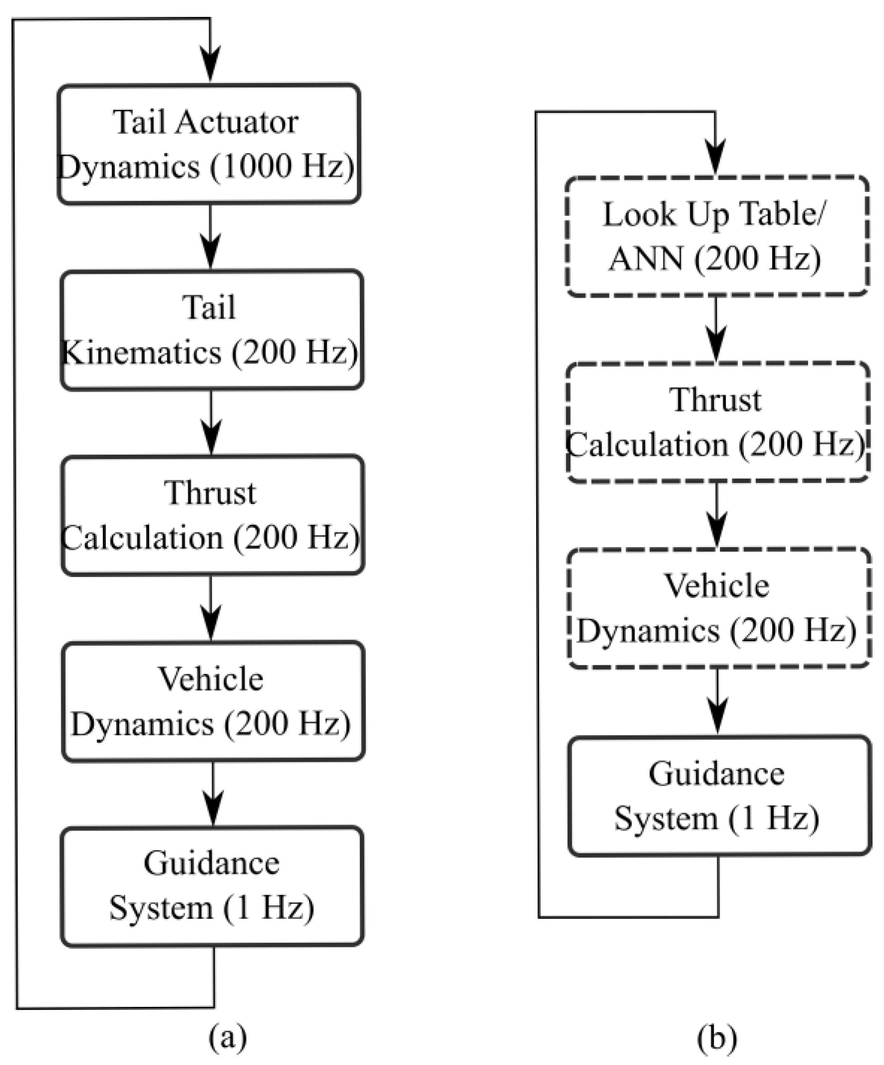
As the results in the previous section demonstrated, mathematical models implementing system identification techniques are able to complete simulations in a fraction of the time required by their corresponding high fidelity, white-box models. As a result, these models are particularly suited to completing investigations into multi-vehicle scenarios. Consequently, the following section will describe the implementation of coordination algorithms based on the behavioural mechanisms of fish to allow a group of BAUVs to be considered self-organizing. The algorithms will be implemented within the LUT and ANN models described in the previous section and a comparison between the results obtained from these models and the original high fidelity model will be made in terms of accuracy and simulation execution time.
In order to successfully operate a group of vehicles within a fully autonomous multi-vehicle scenario a number of different features of the overall system design have to be taken into consideration. These features can be broadly categorized into the following groups: Coordination Methodologies, Communication, Vehicle Control and Dynamics.
The interdependencies and relationships which exist among these features is known as the system architecture and is presented diagrammatically in Figure 12.
Figure 12. System architecture for coordinating multiple BAUV’s autonomously. Design features within the green box relate to design considerations for each of the individual vehicles within the group. Design features within the red box relate to the features required to allow the vehicles within the group to communication and coordinate with one another.
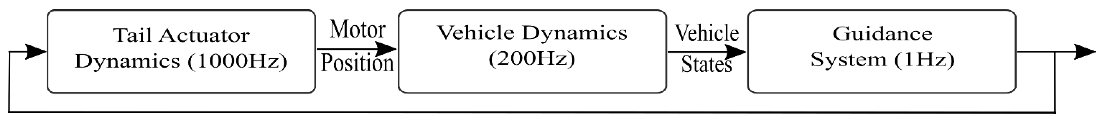
Robotics 05 00002 g012
Within Figure 12, the Vehicle Dynamics and Control section represents the dynamics and kinematics of the RoboSalmon vehicle described in Section 2.2. While for the navigation section, it is assumed that each vehicle’s position is known and represented by a two-dimensional Cartesian coordinate system.
In addition, apparent from Figure 12 is that in order to produce autonomous multi-vehicle coordination, a communication strategy has to be established to allow the individual vehicles within the group to share their relevant positional data. Furthermore, coordination algorithms have to be implemented that are able to process and utilize this information to manoeuvre the vehicles to move in the correct direction.
However, as discussed previously, the underwater milieu presents a number of unique characteristics which makes the implementation of these two design features particularly challenging. Therefore, it is the purpose of the following sections to present the communication protocols and coordination algorithms implemented that take into account these challenges and allow the coordination of a school of BAUVs.
The implementation of a communication strategy within any group scenario is essential to the group’s ability to successfully complete the specified task. However, due to the aforementioned physical limitations of the underwater communication channel, the implementation of a successful communication strategy for multi-vehicle cooperation is particularly challenging. Nonetheless, presently there are three strategies utilized within the underwater acoustic channel: Frequency Division Multiple Access (FDMA), Code Division Multiple Access (CDMA) and Time Division Multiple Access (TDMA) [36]. Evidently, in order to implement these strategies, each of the vehicles would have to be fitted with an acoustic modem. While there are acoustic modems on the market which could fit into the current version of RoboSalmon [37], it is expected that the size of the vehicle would have to be slightly increased to allow further sensing equipment payload to be incorporated within the vehicle.
While each of the above possess their own operational benefits, this paper involves the implementation of a TDMA protocol for facilitating communication among the different vehicles. The TDMA protocol operates by assigning each vehicle within a group a unique timeslot within which it can transmit its data to the other vehicles. Once each vehicle has transmitted its data once, the process is repeated and the cycle continues until the end of the mission [37]. The length of the timeslot, t is dependent on the transmission time of the data and the propagation delay due to the speed of sound in water. The timeslot can be calculated using the following equation:
t = Transmission Time + Maximum Intervehicle Distance 1500
The Transmission Time in the above equation is a constant value based on the size of the data being transmitted (256 bits) and the transmission rate of the acoustic modem (31.2 kbits/s). The second term is known as the propagation delay and determines the maximum time interval required for a packet of data to be transferred between the two vehicles furthest away from one another. As it is not possible to know the exact value of this parameter, a conservative estimation is made based on one of the parameters associated with the coordination algorithms and is discussed below in Section 4.

3.1. Coordination Algorithms

As discussed earlier, one of the main motivations for operating AUVs within multi-vehicle deployments is to allow the collection of data over large spatiotemporal domains. Consequently, the coordination of the vehicles within the group is of critical importance to ensure not only their safe operation but also to ensure that the data collected is done so in an efficient manner. To achieve this, the algorithms implemented will have to ensure that neighbouring vehicles do not collide with one another but also ensure the formation of a group structure moving with a common directionality.
While several coordination methodologies exist that, if implemented, would satisfy the above criteria, the work presented in this paper will once again take inspiration from nature and implement a coordination strategy based on the behavioural mechanisms known to exist within school structures in nature.
These naturally occurring formations have been known to range in size from small groups containing as little as two individuals to immense structures containing millions of fish often moving with remarkable synchronicity [38]. While, initially, debate surrounded the exact mechanism used to explain this phenomenon, Aoki’s work published in 1981 presented a set of behavioural mechanisms that when implemented within a simulation model, successfully imitate the behaviours exhibited by fish within school structures in nature [39].
In his paper, Aoki established that fish must poses three behavioural tendencies in order to produce the schools structures displayed in nature i.e., repulsion, orientation and 
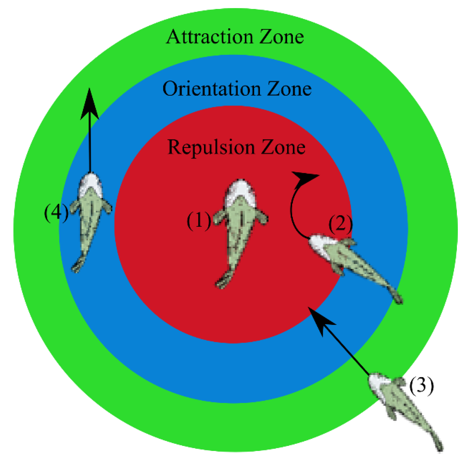
attraction. The specific mechanism presented in Aoki’s paper to trigger the above behaviours is to assign three concentric circles of variable size to each individual and depending on which of these zones is occupied by its nearest neighbours, the individual in the centre will manoeuvre in either a repulsive, orientating or attractive manner as shown in Figure 13.
Figure 13. Graphical representation of behavioural mechanisms of fish within school structures. The diagram demonstrates how Fish (2), (3) and (4) would manoeuvre with reference to Fish (1). Fish (2) occupies the Repulsion Zone so it would look to move away from Fish (1). Fish (3) occupies the Attraction Zone and would therefore look to move towards Fish (1). Fish (4) occupies the Orientation Zone and would therefore align its heading angle with that of Fish (1).
Robotics 05 00002 g013
Therefore, it is believed that this mechanism can be adopted and implemented as a coordination strategy for the coordinated movement of multiple vehicles. However, it is apparent from Figure 13 that in order to implement the above mechanism, the individual vehicles within the group have to communicate their positional and heading data to the other vehicles within the group. As presented in [20], the RoboSalmon vehicle is equipped with an Inertial Measurement Unit (IMU) containing a combination of accelerometers and gyroscopes. Consequently, dead reckoning techniques could be implemented to integrate the signals from these sensors to obtain each vehicle’s positional and orientation data. While dead reckoning techniques produce positional error growth [40], for the purposes of the investigations completed in this paper, the influence of these errors on the coordination algorithms have not been taken into consideration. As discussed, this occurs through the transmission of data using acoustic communication methods and adopting a TDMA protocol.

3.2. Implementation of Coordination Algorithms

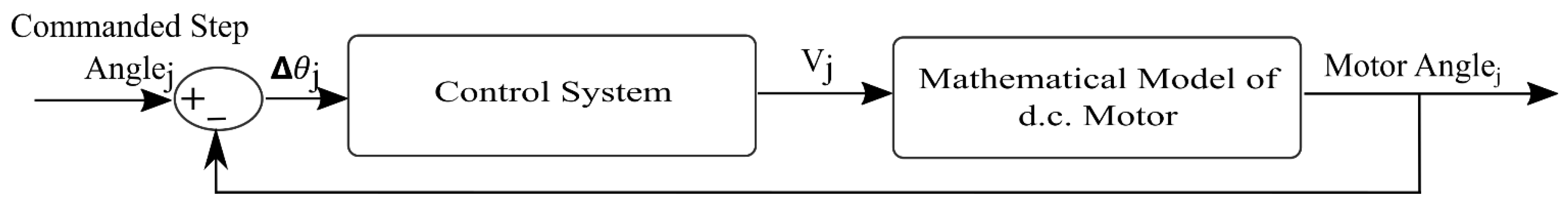
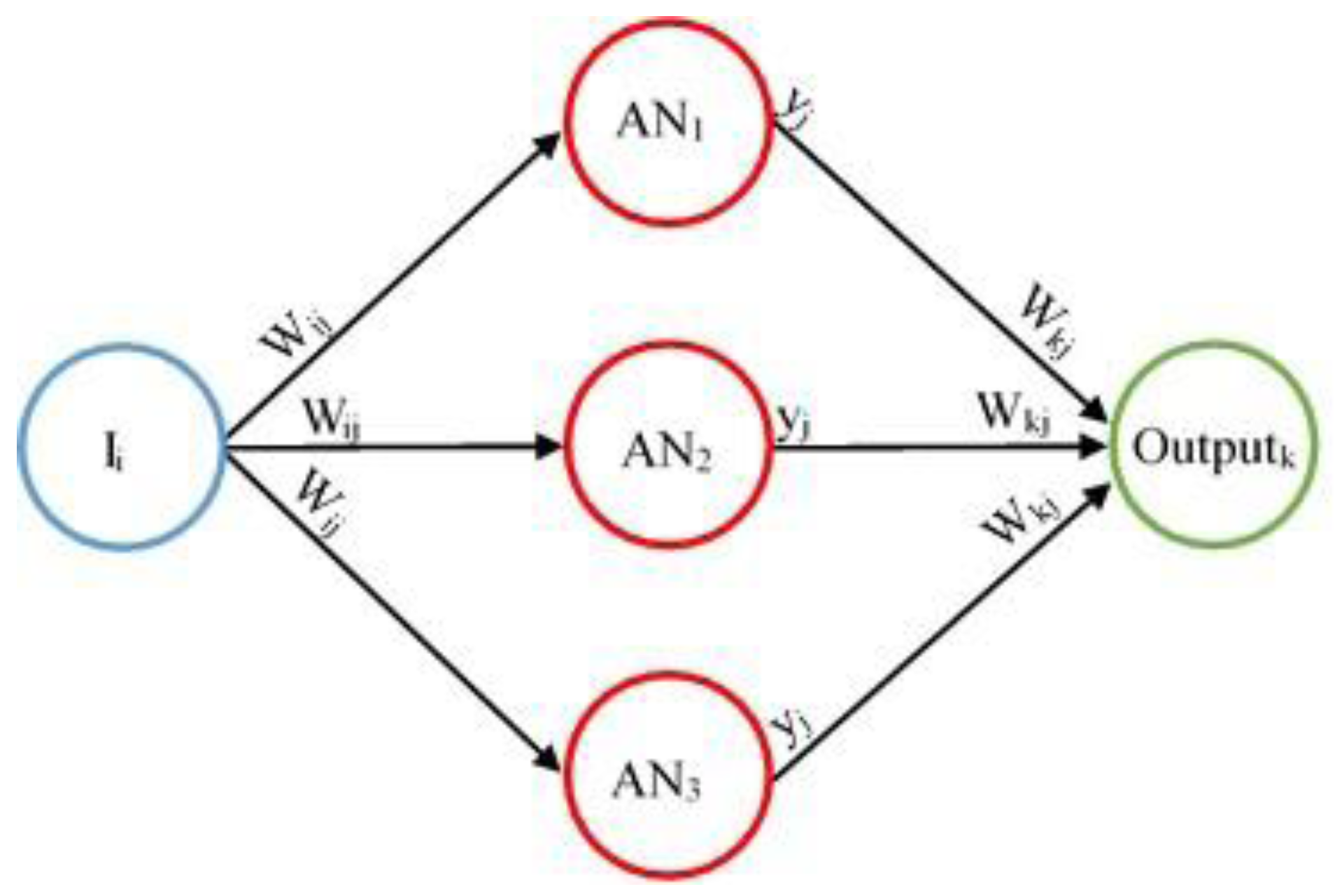
The controller implemented within the Guidance System (Figure 2) to alter the heading angle of each vehicle requires a desired heading angle as an input. Consequently, the equations implemented to produce either a repulsive, orientating or attractive manoeuvre from each vehicle are required to produce an angular value based on the positional and heading data of its nearest neighbours as well as the behavioural zone which the neighbouring vehicles are occupying.

3.2.1. Repulsive Behaviour

The repulsive behaviour of each vehicle within the group has to ensure that the vehicle will manoeuvre in such a way as to avoid colliding with its nearest neighbour. The equation implemented to achieve this behaviour is shown below in Equation (9).
ψ LOS = ψ V   ±   π 4
where ψ LOS represents the desired heading angle (radians) which is input to the controller within the guidance system and ψ V is the present heading angle of the vehicle. The decision of whether to add or subtract the 45° depends on the relative position between the two vehicles in question.

3.2.2. Orientating Behaviour

On the other hand, the orientating behaviour has to result in each vehicle aligning its heading angle with that of its nearest neighbours and the equation implemented within the algorithm to achieve this is shown below:
ψ LOS = 1 I NN NN = 1 I NN ψ NN

3.2.3. Attractive Behaviour

Finally, the attractive behaviour of each vehicle has to result in a manoeuvre that results in each vehicle reducing its distance to its neighbouring vehicles. This is achieved by creating a point in space which is equal to the average x and y positions of each vehicles nearest neighbours. The equations implemented to complete this task is shown below:
x d = 1 I NN NN = 1 I NN x NN
y d = 1 I NN NN = 1 I NN y NN
where x N N and y N N represent the x and y positions of nearest neighbours, respectively. These positions are then used to evaluate the required heading angle,   ψ L O S of the vehicle to manoeuvre in the direction of its nearest neighbour using the equation shown below.

3.2.4. Structure of Coordination Algorithm

The decision process to determine which of the above equations is used and its relationship with the communication protocol described in Section 3.1 is known as the algorithms structure and is presented below in Figure 14.
Figure 14. Algorithm structure.
Robotics 05 00002 g014
Equations (9)–(12) and the structure presented above represent the coordination algorithm implemented based on the behavioural mechanisms of fish within school structures. The following section presents results demonstrating the effectiveness of the above strategy to coordinate multiple BAUVs form a school structure.

4. Results

In the work, presented in this paper, a deployment of 12 vehicles is simulated for two different behavioural zones sizes. The maximum number of nearest neighbours that each vehicle could take into consideration is set to six based on the results from the work completed in [41,42]. Furthermore, as demonstrated by Equation (8), the time slot assigned to each vehicle to communicate its relevant data to the remaining vehicles is predetermined and is based on the transmission time of the data and the propagation delay. While the transmission time is constant at 0.008 s, the propagation delay is dependent on the maximum distance between two vehicles within the group. However, since this value cannot be determined and in actual fact varies throughout the simulation, a conservative value for the maximum distance between two vehicles has been selected to be double the size of the attraction zone utilised within the simulation. Finally, the size of the behavioural zones have been selected to ensure that the minimum inter-vehicle distances across the deployment are such that hydrodynamic interactions are negligible based on the results of [43]. The above parameters are summarized below in Table 6.
Table 6. Simulation parameters.
ParameterValue
Deployment Size12 Vehicles
Number of Nearest Neighbours6
Small Behavioural Zone Sizes2, 8, 50 m
Large Behavioural Zone Sizes10, 20, 60 m
Time Slot Size—Small Behavioural Zone0.07 s
Time Slot Size—Large Behavioural Zone0.08 s
Simulations utilizing the above parameters where completed for the three models discussed in this paper: the original high fidelity model, the LUT and ANN models. The following section will present the results from these simulations in terms of the ability of the algorithms to form a group structure but also to analyse the performance of the reduced models compared to the high fidelity model.
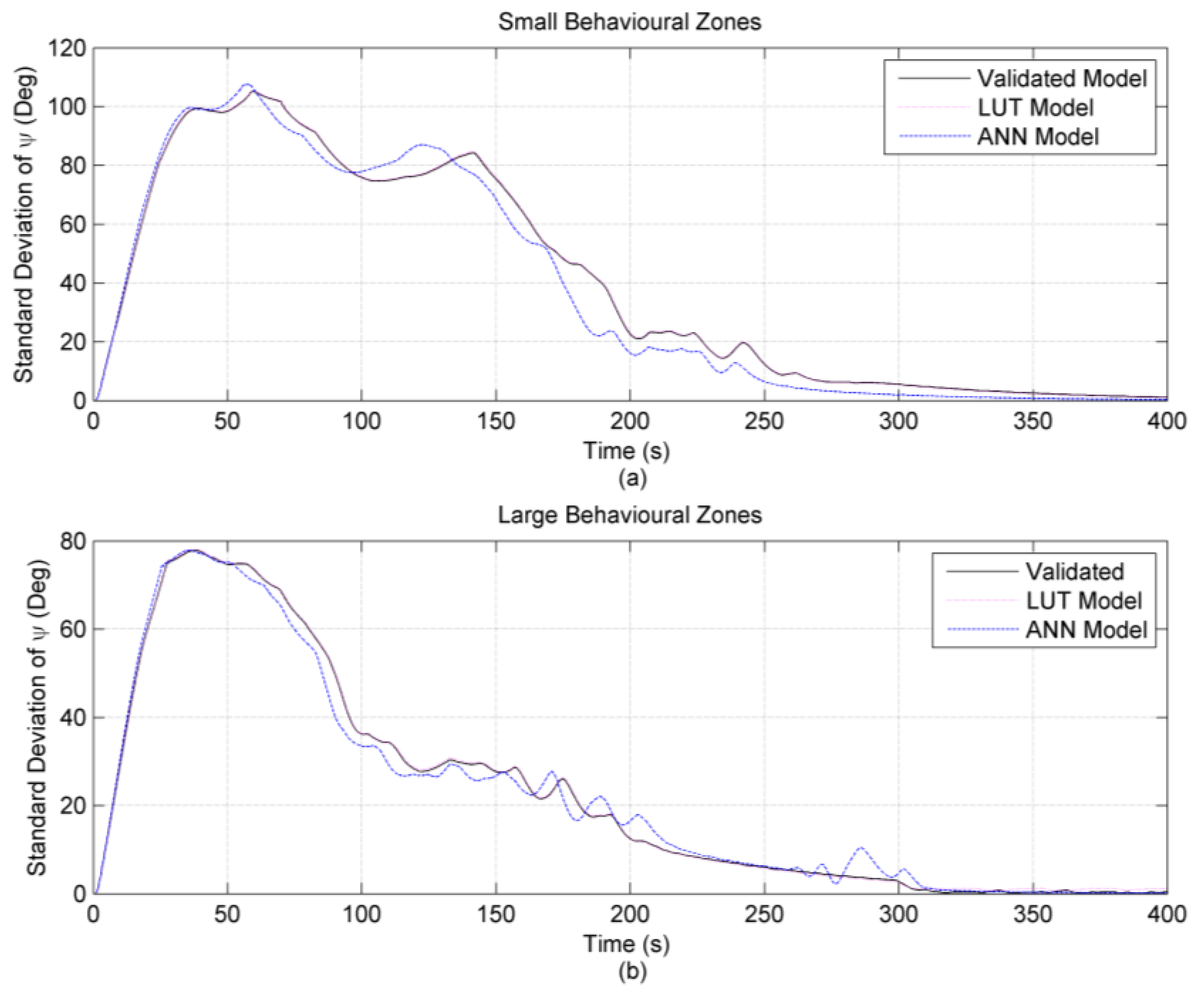
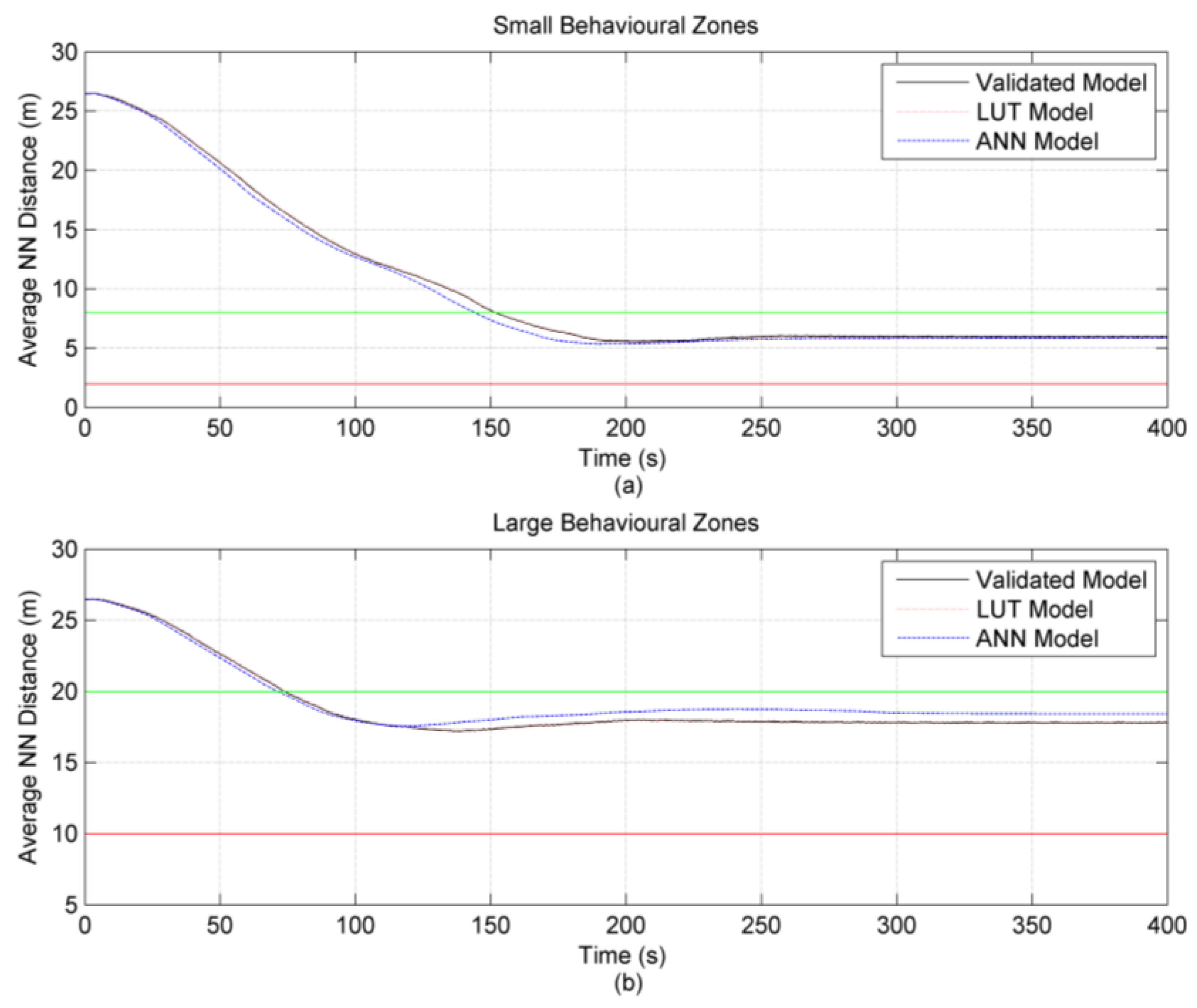
In order to determine whether or not the coordination algorithms have been successful, the variation in the average heading angle of the group was calculated using the standard deviation metric. Consequently, if the standard deviation calculated converges to a relatively small value, then it can be concluded with confidence that all the vehicles within the group are moving with a common directionality. However, to definitively demonstrate that the algorithms have been successful, the average distance to each vehicles nearest neighbours should also converge to be within the boundaries of the orientation zone. Therefore, the above metrics where calculated for the results produced from each of the three models discussed in this work and the results are presented below in Figure 15 and Figure 16.
Figure 15 and Figure 16 clearly demonstrate that for each of the three models, the standard deviation and average nearest neighbour metrics behave as expected and converge to a steady state value. This suggests that the coordination algorithms have been successful in promoting the formation of a self-organizing group. Inspecting Figure 15 and Figure 16 more closely, it also becomes apparent that for the simulations involving the smaller behavioural zones, the time to convergence is greater when compared to the simulations involving the larger behavioural zones. This behaviour is yet again expected as the initial starting positions are the same for both scenarios and therefore, the time taken for individuals to start occupying one another’s orientations zones will be less when the behavioural zone sizes are larger.
Figure 15. Comparison between results obtained for validated model, LUT model and ANN model for the standard deviation of heading angle of the group. The figure also presents the results for two different behavioural zone sizes. (a) Small Behavioural Zone Sizes (Table 6); (b) Large Behavioural Zone Sizes (Table 6).
Robotics 05 00002 g015
Figure 16. Comparison between results obtained for original model, LUT model and ANN model for the standard deviation of heading angle of the group. The figure also presents the results for two different behavioural zone sizes. (a) Small Behavioural Zone Sizes (Table 6); (b) Large Behavioural Zone Sizes (Table 6).
Robotics 05 00002 g016
In relation to the accuracy of the reduced fidelity models, the above metrics cannot be used to compare the different models. The reason that this is the case is that, although the standard deviation of the heading angle converges to zero for each model, the results from the reduced fidelity models might have an entirely different average heading angle to that of the validated model and therefore, the group may be converge to a different heading angle. Nevertheless, the above figures would suggest that the results produced from the ANN model are slightly less accurate than that of the results produced from the LUT model. This becomes apparent by inspecting Figure 15 where the evolution of the standard deviation metric is noticeable different for the ANN model when compared with the validated model and LUTs results.
However, in order to accurately quantify the discrepancy between the different models, the Theil’s Inequality Coefficient (TIC) was calculated again for each of the six states presented in Table 2 for the results produced from the multi-vehicle simulations. The results are presented below in Table 7.
Table 7. Average TIC values obtained from comparison of simulations implementing the large and small behavioural zones.
Body and Earth Fixed VariablesSmall Behavioural ZonesLarge Behavioural Zones
Artificial Neural NetworkLook Up TableArtificial Neural NetworkLook Up Table
Surge0.10230.05150.07990.0399
Sway0.24750.16160.21680.1375
Roll0.46040.31230.44470.3185
X-Pos0.04030.01170.02900.0061
Y-Pos0.07710.03420.09320.0447
Heading Angle0.21470.1200.19780.1317
The results presented in Table 7 clearly demonstrate that, regardless of the behavioural zone sizes implemented, the TIC values are greater for the comparison between the validated model and ANN model than they are for the comparison between the LUT model and the validated model. This would support the findings discussed above from the visual inspection of Figure 15.
The reason that the ANN model is not as accurate as the LUT is due to the way in which the neural network was trained. The target data supplied to the ANN for training purposes was the evolution caudal fins position throughout one second corresponding to a specific tail centre deflection angle. In order to ensure the evolution of the caudal fin’s position throughout the vehicle’s entire operational range was supplied to the ANN, only caudal fin positions relating to tail centre deflection angles in five degree intervals where supplied to the network. As a result, the ANN produced a mapping which would be accurate for tail centre deflection angles starting at −90° and ending at 90° in five degree intervals. This was disguised in the results for the open loop manoeuvres where the tail centre deflections angles utilised (Table 3) coincided with the same angles for which training data were supplied to the ANN.
However, for the simulations involving multi-vehicle scenarios, the commanded tail centre deflection angles could be any value between −90 and 90. Therefore, the ANN was producing values for the caudal fin’s position which it had not been specifically trained to produce and was instead, relying on the mapping obtained during the training phase to be sufficiently accurate.
Furthermore, while the ANN was only supplied training data at five degree intervals, the LUTs constructed contained data for the caudal fins position at one degree intervals. Consequently, the look table model only had to interpolate between one degree intervals in tail centre deflection angle whereas, the ANN was essentially interpolating over five degree intervals.
By comparing the results from Table 4 and Table 7, it is also apparent that the TIC values has increased for both the LUT model and ANN model. The reason for this can be explained by the nature of the open loop manoeuvres, whereby the tail centreline is deflected to a particular value where it remains for a considerable period of time. Whereas, within the multi-vehicle scenario, the tail centreline will be transitioning between various angles at a frequency of 1 Hz. Therefore, the fact that more transient behaviour exists within the multi-vehicle simulations would suggest that the system identification techniques employed to represent the transient behaviour are less accurate than those employed to evaluate the steady-state behaviour.
Table 7 also demonstrates that the state parameter which has the greatest discrepancy is the roll rate, with a maximum value of 0.4604. However, closer analyses of the difference between the results produced from the models for this parameter demonstrates that the TIC of 0.4604 value is equivalent to a maximum discrepancy of 6.33°/s.
However, as well as analysing the accuracy of the models for the multi-vehicle simulations, the run time performance of the models has been evaluated. The multi-vehicle simulations evaluated 400 s worth of data and the original model required approximately 40 min to complete, the LUT model required approximately 3.8 min while the ANN model required approximately 4.2 min.
Finally, the overall difference in the results produced from the three plots can be visually analyzed by inspecting the trajectory plots obtained from the results as shown below in Figure 17.
Figure 17. Comparison of trajectory plots obtained from the three models. Black trajectory represents validated model, blue line represents the ANN model and the red line represents the LUT Model. (a) Small Behavioural Zone Sizes (Table 6); (b) Large Behavioural Zone Sizes (Table 6).
Robotics 05 00002 g017
Although Figure 17 demonstrates that there are differences between the reduced fidelity models and the validated model, the magnitude of the discrepancy is small in comparison to the improvement in the simulation execution time achieved.

5. Conclusions

The work presented in this paper has defined the operational benefits of being able to deploy a self-coordinating group of AUVs for oceanic monitoring purposes, the challenges associated with doing so as well as the current state of the art in the deployment of groups of AUVs.
The paper has also demonstrated the benefits associated with implementing system identification techniques to replace complex functionality within high fidelity mathematical models to allow a drastic reduction in the simulation execution time while still producing results that are representative of the dynamics of the RoboSalmon vehicle. However, the results also demonstrated that of the two system identification techniques implemented, the model implementing LUTs was slightly more accurate when compared to the results obtained from the ANN model.
Furthermore, this paper has also presented the feasibility of implementing a decentralized coordination algorithm based on the behavioural mechanisms of fish to allow a group of BAUVs to be considered self-organizing. The results also demonstrated the ability of the algorithms to coordinate the vehicles to manoeuvre with specific inter-vehicle distances and therefore the algorithms could be implemented to allow a group of BAUVs to completed large-scale spatiotemporal data collection.
Therefore, in summarizing, the results produced in this paper have demonstrated the ability to implement system identification techniques to produce low fidelity mathematical models that dramatically reduce simulation execution time while maintaining an accurate representation of RoboSalmon’s dynamics. As a result, these models are able to produce more efficient simulations when investigating multi-vehicle scenarios. However, the results also demonstrated that of the two system identification techniques implemented, the LUT model was not only more accurate but was also capable of completing simulations quicker than the ANN model.

Acknowledgments

The financial support for the work completed in this paper has been provided by Engineering and Physical Sciences Research Council (EPSRC) through the award of a Doctoral Training Grant (DTG).

Author Contributions

The research completed to attain the results provided in this paper and the initial drafting of the above report was completed by Jonathan McColgan. Euan McGookin provided insight and advice throughout the completion of the research as well as reviewing and providing contributions during the writing phase of this paper.

Conflicts of Interest

The authors declare no conflict of interest.

References

  1. Miller, S.; Spoolman, G. Climate and Biodiversity. In Environmental Science; Brooks/Cole: Belmont, CA, USA, 2010. [Google Scholar]
  2. Copley, J. Just How Little Do We Know about the Ocean Floor. 2014. Available online: http://www.scientificamerican.com/article/just-how-little-do-we-know-about-the-ocean-floor/ (accessed on 15 October 2015).
  3. Redfield, S. Cooperation between Underwater Vehicles. In Marine Robot Autonomy; Springer-Verlag: New York, NY, USA, 2013; pp. 257–286. [Google Scholar]
  4. Mohamed, N.; Jawhar, I.; Al-Jaroodi, J.; Zhang, L. Monitoring underwater pipelines using sensor networks. In Proceedings of the 2010 12th IEEE International Conference on High Performance Computing and Communications (HPCC), Melbourne, Australia, 1–3 September 2010; pp. 346–353.
  5. Stacy, D. Deep-Sea Explorers Angle to Solve Mystery of Missing Malayasian Airliner. Wall Street J. 2014, 8, 1–9. [Google Scholar]
  6. Lapierre, L. Underwater Robots Part I: Current systems and problem pose. In Mobile Robotics—Towards New Applications; Advanced Robotic Systems International: Mammendorf, Gernmany, 2006; pp. 310–334. [Google Scholar]
  7. Kaminski, C.; Crees, T.; Ferguson, J.; Forrest, A.; Williams, J.; Hopkin, D.; Heard, G. 12 Days Under Ice—An Historic AUV Deployment in the Canadian High Arctic. In Proceedings of the 2010 IEEE/OES Autonomous Underwater Vehicles, AUV 2010, Monterey, CA, USA, 1–3 September 2010.
  8. Griffiths, G.; Jamieson, J.; Mitchell, S.; Rutherford, K. Energy storage for long endurance AUVs. In Proceedings of the ATUV Conference, iMarEST, London, UK, 16–17 March 2004.
  9. Petillo, S.; Schmidt, H.; Balasuriya, A. Constructing a distributed AUV network for underwater plume-tracking operations. Int. J. Distrib. Sens. Netw. 2012, 2012, 191235. [Google Scholar] [CrossRef]
  10. Fiorelli, E.; Leonard, N.E.; Bhatta, P.; Paley, D.A.; Bachmayer, R.; Fratantoni, D.M. Multi-AUV control and adaptive sampling in Monterey Bay. IEEE J. Ocean. Eng. 2006, 31, 935–948. [Google Scholar] [CrossRef]
  11. Sotzing, D.M.; Lane, C.C. Improving the coordination efficiency of limited-commuication multi-autonomous underwater vehicle operations using a multiagent architecture. J. F. Robot. 2010, 27, 412–429. [Google Scholar] [CrossRef]
  12. Diamant, R.; Lampe, L. Spatial reuse time-division multiple access for broadcast Ad Hoc underwater acoustic communication networks. IEEE J. Ocean. Eng. 2011, 36, 172–185. [Google Scholar] [CrossRef]
  13. Murray-Smith, D.J. Experimental Modelling: System Identification, Parameter Estimation and Model Optimsation Techniques. In Modelling and Simulation of Integrated Systems in Engineering; Woodhead Publishing: Cambridge, UK, 2012. [Google Scholar]
  14. Mazlan, A.N.A.; McGookin, E. Modelling and Control of a Biomimetic Autonomous Underwater Vehicle. In Proceedings of the International Conference on Control, Automation, Robotics & Visions, Guangzhou, China, 5–7 December 2012; pp. 88–93.
  15. Wu, Z.; Yu, J.; Tan, M.; Zhang, J. Kinematic comparison of forward and backward swimming and maneuvering in a self-propelled sub-carangiform robotic fish. J. Bionic Eng. 2014, 11, 199–212. [Google Scholar] [CrossRef]
  16. Watts, C.; McGookin, E.; Macauley, M. Modelling and Control of a Biomimetic Underwater Vehicle with a Tendon Drive Propulsion System. In Proceedings of the Oceans 2007—Europe, Aberdeen, UK, 18–21 June 2007; pp. 1–6.
  17. Watts, C.; McGookin, E. Modeling and Simulation of a Biomimetic Underwater Vehicle. In Proceedings of the Summer Simulation Multi-Conference, Edinburgh, UK, 2008.
  18. Takada, Y.; Koyama, K.; Usami, T. Position Estimation of Small Robotic Fish Based on Camera Information and Gyro Sensors. Robotics 2014, 3, 149–162. [Google Scholar] [CrossRef]
  19. Watts, C.M.; McGookin, E.W. Surge Performance of an Underwater Vehicle with a Biomimetic Tendon Drive Propulsion System. J. Eng. Marit. Environ. 2013, 228, 315–330. [Google Scholar] [CrossRef]
  20. Mazlan, A.N.A. A Fully Actuated Tail Propulsion System for a Biomimetic Autonomous Underwater Vehicle; University of Glasgow: Glasgow, UK, 2015. [Google Scholar]
  21. Hemelrijk, C.K.; Hildenbrandt, H. Self-organized shape and frontal density of fish schools. Ethology 2008, 114, 245–254. [Google Scholar] [CrossRef]
  22. Couzin, I.D.; Krause, J.; James, R.; Ruxton, G.D.; Franks, N.R. Collective memory and spatial sorting in animal groups. J. Theor. Biol. 2002, 218, 1–11. [Google Scholar] [CrossRef] [PubMed]
  23. Huth, A.; Wissel, C. The Simulation of the Movement of Fish Schools. J. Theor. Biol. 1991, 156, 365–385. [Google Scholar] [CrossRef]
  24. Sherman, J.; Davis, R.E.; Owens, W.B.; Valdes, J. The autonomous underwater glider "Spray". IEEE J. Ocean. Eng. 2001, 26, 437–446. [Google Scholar] [CrossRef]
  25. Simonetti, P. Slocum Glider: Design and 1991 Field Trials; Woods Hole Oceanographic Institution: Woods Hole, MA, USA, 1992. [Google Scholar]
  26. Boston, E. BIOSwimmer: Changing the Underwater Inspection Game; Boston Engineering: Boston, MA, USA, 2014. [Google Scholar]
  27. Geo-Matching, "Iver2-580". Available online: http://www.geo-matching.com/products/id1973-iver2-580.html (accessed on 16 December 2015).
  28. Geo-Matching, “Bluefin-9M”. Available online: http://www.geo-matching.com/products/id1951-bluefin-9m.html (accessed on 16 December 2015).
  29. Fish, F.E.; Kocak, D.M. Biomimetics and Marine Technology: An Introduction. Mar. Technol. Soc. J. 2011, 45, 8–13. [Google Scholar] [CrossRef]
  30. Lighthill, M.J. Note on the swimming of slender fish. J. Fluid Mech. 1960, 9, 305–317. [Google Scholar] [CrossRef]
  31. Fossen, T.I. Guidance and Control of Ocean Vehicles; John Wiley & Sons: Chichester, UK, 1994. [Google Scholar]
  32. Sargent, R.G. Validation and verification of simulation models. In Proceedings of the Winter Simul. Conference WSC, Washington, DC, USA, 9–12 December 2007; pp. 124–137.
  33. Mathworks, “Profiling for Improving Performance”. Available online: http://uk.mathworks.com/help/matlab/matlab_prog/profiling-for-improving-performance.html (accessed on 8 May 2015).
  34. Gurney, K. Neural Network—An overview. In An Introduction to Neural Networks; Taylor & Francis Group: London, UK, 1997; pp. 1–6. [Google Scholar]
  35. Bishop, C. Statistical Pattern Recognition. In Neural Networks for Pattern Recognition; University Press Inc.: New York, NY, USA, 1995; pp. 1–28. [Google Scholar]
  36. Burrowes, G.E.; Brown, J.; Khan, J.Y. Adaptive Space Time—Time Division Multiple Access ( AST-TDMA ) Protocol for an Underwater Swarm of AUV’s. In Proceedings of the OCEANS Conference, Bergen, Norway, 10–14 June 2013; pp. 1–10.
  37. Evo Logics, S2CR 48/78 Product Information. 2014. Available online: http://www.evologics.de/files/DataSheets/EvoLogics_S2CR_4878_Product_Information.pdf (accessed on 16 December 2015).
  38. Parrish, J.K.; Viscido, S.V. Traffic rules of fish schools: A review of agent-based approaches. In Self-Organisation and Evolution of Social Systems; Cambridge University Press: Cambridge, UK, 2005; pp. 50–80. [Google Scholar]
  39. Aoki, I. A Simulation Study on the Schooling Mechanism in Fish. Bull. Jpn. Soc. Sci. Fish. 1981, 48, 1081–1088. [Google Scholar] [CrossRef]
  40. Paull, L.; Saeedi, S.; Seto, M.; Li, H. AUV navigation and localization: A review. IEEE J. Ocean. Eng. 2014, 39, 131–149. [Google Scholar] [CrossRef]
  41. McColgan, J.; McGookin, E.; Mazlan, A.N.A. Analysis of the Group Structure of a School of Biomimetic AUVs Coordinated Using Nearest Neighbour Principles. In Proceedings of the 6th International Conference on Automation, Robotics and Applications, Queenstown, New Zealand, 17–19 February 2015; pp. 312–317.
  42. McColgan, J.; McGookin, E.W.; Mazlan, A.N.A. A Low Fidelity Mathematical Model of a Biomimetic AUV for Multi-Vehicle Cooperation. In Proceedings of the OCEANS 2015, Genoa, Italy, 18–21 May 2015.
  43. Daghooghi, M.; Borazjani, I. The Hydrodynamic Advantages of Synchronized Swimming in a Rectangular Pattern. Bioinspir. Biomim. 2015, 10, 1–23. [Google Scholar] [CrossRef] [PubMed]

