Reconfiguration Analysis of an RRRRS Single-Loop Mechanism

Abstract

The paper deals with the reconfiguration analysis of the single-loop variable degree-of-freedom (DOF) RRRRS mechanism composed of five links connected by four revolute (R) joints and one spherical (S) joint. The mechanism may show two modes of motion: one-DOF and two-DOF motion. In the paper, a classical vector procedure is used to obtain the quartic motion equation (QME) that allows one to inspect the nature of the motion. In general, the solutions of the QME provide the one-DOF motion of the mechanism except when all the coefficients of the equation vanish. In this case, the mechanism undergoes the two-DOF motion. The motion of the mechanism built according to two specific architectures was analyzed by the numerical solutions of the QME and with the help of the solid model of the mechanism. It is revealed for the first time that the perpendicular architecture has one 2-DOF motion and two 1-DOF motion modes.

1. Introduction

The paper deals with the reconfiguration analysis of a variable-degree-of-freedom (DOF) single-loop mechanism. Variable-DOF mechanisms (also kinematotropic mechanisms), are a class of reconfigurable mechanisms and one type of multi-mode mechanisms. Research in reconfigurable mechanisms dated back to 1996 when the first paper was published [1]. Since then, the researchers have been developing several approaches both for the type synthesis of these mechanisms [2,3,4,5,6,7,8] and for their kinematic analysis (a.k.a., reconfiguration analysis), [9,10,11,12,13,14,15,16,17,18,19,20,21,22,23,24,25,26,27]. Indeed, despite of the kinematic analysis of conventional mechanisms, these mechanisms pose the new fundamental problem of finding all the possible motion modes and to identify the transition configurations. In general, this requires solving a set of loop-vector or constraint (polynomial) equations. The solutions can be obtained via traditional vector methods but also with the help of algebraic, numerical algebraic geometry and computer algebra. For example, focusing only on single-loop mechanisms, in [11] the algorithm for the inverse kinematics of the serial 6R mechanism using the Study’s kinematic mapping was adopted to deal with the kinematic analysis of single-loop reconfigurable 7R mechanism with multiple operation modes. In [12], the analytical inverse kinematic solution of a 4R2P open chain is adopted to analyze the 5R2P linkage for a given driving joint angle. From the analysis, three operation modes were obtained. In [13], a different approach was followed. The reconfigurability property of the Bennett plano-spherical linkage (closed-loop 6R linkage) has been revealed by the variation of the order of the motion-screw system without writing down a set of polynomial equations. Very recently, the reconfiguration analysis of a novel 7R single-loop variable-DOF mechanism, obtained from a general variable-DOF single-loop 7R spatial mechanism and a plane symmetric Bennett joint 6R mechanism for circular translation, has been carried out in the configuration space by solving a set of kinematic loop equations based on dual quaternions and the natural exponential function substitution using tools from algebraic geometry. The analysis shows that the mechanism has five motion modes [27]. That paper continues the work presented in [26] where the set of six polynomial kinematic loop equations were obtained and solved in a similar manner for a 7R multimode spatial mechanism.

In this paper the reconfiguration analysis of a single-loop, variable-DOF RRRRS mechanism is carried out. The mechanism can be considered a special class of the spatial single-loop 7R mechanism with three of the seven revolute joints collapsed into the spherical joint. This mechanism was firstly proposed in [11] using a construction approach and then also found in [7] by the method of intersection of surfaces generated by kinematic dyads, then providing a general theoretical proof of the local mobility by the geometrical algebra method. The motivation of this work is to carry out the reconfiguration analysis of this mechanism that was not previously presented. The main idea of the analysis is to use the inverse kinematic procedure of the serial chain 3R in order to find the quartic motion equation (QME). Solutions of the QME were investigated numerically and with the help of the solid model of the mechanism built according to two specific architectures. The paper is organized as follows. In Section 2 the description of the mechanism is given and the reference systems are set according to the Denavit-Hartenberg standard convention. In Section 3 the QME is obtained from the loop-vector equation of the mechanism. The QME is a polynomial equation written in terms of one joint angle with its coefficients depending on an other joint angle and on the links parameters of the mechanism. In Section 4 the inspection of the QME was carried out for two specific architectures of the mechanism. Finally, in Section 5 the conclusions of the work are drawn.

2. Description of the RRRRS Variable-DOF Mechanism

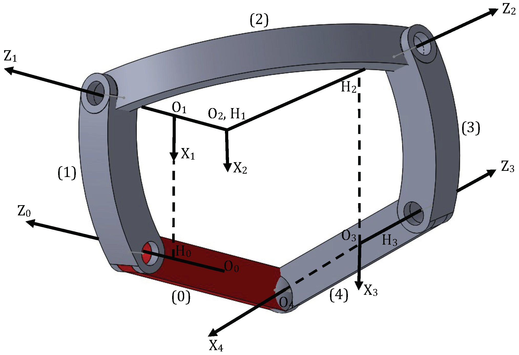
The mechanism under study is a single-loop formed by five links with four revolute (R) joints and a spherical (S) joint. The mechanism is shown in Figure 1. All the links can move according to the constraints except the link (0) that has to be considered as fixed. Figure 1 shows the reference systems attached to the links according to the Denavit-Hartenberg (D-H) standard convention. Briefly, the convention is here for the sake of clearity. The $Z_i$-axis is along the axis of joint $(i+1)$. The $X_i$-axis is along the common perpendicular between $Z_{i-1}$- and $Z_i$-axes. $O_i$ is the intersection of $X_i$- and $Z_i$-axes whilst $H_{i-1}$ is the intersection of $Z_{i-1}$- and $X_i$-axes. The link parameters of link i are: ${\theta }_i$: the angle between $X_{i-1}$- and $X_i$-axes measured from $X_{i-1}$-axis to $X_i$-axis about $Z_{i-1}$-axis; $d_i$: the distance between $O_{i-1}$ and $H_{i-1}$ measured from $X_{i-1}$-axis to $X_i$-axis along $Z_i$-axis; ${\alpha }_i$: the twist angle between $Z_{i-1}$- and $Z_i$-axes measured from $Z_{i-1}$-axis to $Z_i$-axis about $Z_{i-1}$-axis; $a_i$: the distance between $H_{i-1}$ and $O_i$ measured from $Z_{i-1}$-axis to $Z_i$-axis along $X_i$-axis.

3. Kinematic Analysis

Consider the single-loop mechanism in Figure 1. We may write the vector loop equation as:

$${\mathbf{o}}_{0,1}+{\mathbf{o}}_{1,2}+{\mathbf{o}}_{2,3}+{\mathbf{o}}_{3,4}+{\mathbf{o}}_{4,0}=\mathbf{0}$$

(1)

where ${\mathbf{o}}_{i-1,i}=\overrightarrow{O_{i-1}{O}_i}$. Equation (1) can be re-written as:

$$({\mathbf{o}}_{0,4}-{\mathbf{o}}_{0,1})-{\mathbf{o}}_{1,2}={\mathbf{o}}_{2,3}+{\mathbf{o}}_{3,4}$$

(2)

where $({\mathbf{o}}_{0,4}-{\mathbf{o}}_{0,1})={\mathbf{o}}_{1,4}$. Then, vectors in Equation (2) can be expressed in the reference system attached to the link 2 such that:

$$\mathbf{l}=\left(\begin{array}{c}{l}_1\\ l_2\\ l_3\end{array}\right)=({}^2{\mathbf{o}}_{1,4}-{{}^2\mathbf{o}}_{1,2})=({{}^2\mathbf{o}}_{2,3}+{{}^2\mathbf{o}}_{3,4})=\mathbf{r}=\left(\begin{array}{c}{r}_1\\ r_2\\ r_3\end{array}\right).$$

(3)

Vectors in Equation (3) are:

$$\begin{array}{c}\hfill {}^2{\mathbf{o}}_{1,4}={}^0{\mathbf{R}}_2^T({\mathbf{o}}_{1,4})={}^1{\mathbf{R}}_2^T\left(\begin{array}{c}\tilde{x}\\ \tilde{y}\\ \tilde{z}\end{array}\right),{{}^2\mathbf{o}}_{1,2}=\left(\begin{array}{c}{a}_2\\ q_2{d}_2\\ p_2{d}_2\end{array}\right),{{}^2\mathbf{o}}_{2,3}=\left(\begin{array}{c}{a}_3{c}_{{\theta }_3}\\ a_3{s}_{{\theta }_3}\\ d_3\end{array}\right),{{}^2\mathbf{o}}_{3,4}={{}^2\mathbf{R}}_3\left(\begin{array}{c}{a}_4{c}_{{\theta }_4}\\ a_4{s}_{{\theta }_4}\\ d_4\end{array}\right).\end{array}$$

In the foregoing equations ${}^{i-1}{\mathbf{R}}_i$ is the orientation matrix of the reference system i with respect to the reference system $i-1$, $p_i=c_{{\alpha }_i}$, $q_i=s_{{\alpha }_i}$ and $c_{{\theta }_i}=cos({\theta }_i)$, $s_{{\theta }_i}=sin({\theta }_i)$, ($i=1,\cdots ,4$). $\tilde{x}$, $\tilde{y}$, $\tilde{z}$ are the coordinates of the spherical joint ($O_4$) with respect to $O_1$ and are expressed in the reference system attached to the link 1. We have:

$$\begin{array}{c}\hfill {}^1{\mathbf{o}}_{1,4}=\left(\begin{array}{c}\tilde{x}\\ \tilde{y}\\ \tilde{z}\end{array}\right)={\mathbf{R}}_1^T({\mathbf{o}}_{0,4}-{\mathbf{o}}_{0,1})=\left(\begin{array}{ccc}{c}_{{\theta }_1}& s_{{\theta }_1}& 0\\ -p_1{s}_{{\theta }_1}& p_1{c}_{{\theta }_1}& q_1\\ q_1{s}_{{\theta }_1}& -q_1{c}_{{\theta }_1}& p_1\end{array}\right)\left(\begin{array}{c}x-a_1{c}_{{\theta }_1}\\ y-a_1{s}_{{\theta }_1}\\ z-d_1\end{array}\right),\end{array}$$

where x, y, z are the coordinates of the spherical joint ($O_4$) with respect to $O_0$ and are expressed in the fixed reference system attached to the link 0. The foregoing equation leads to:

$$\begin{array}{c}\hfill \tilde{x}=x{c}_{{\theta }_1}+y{s}_{{\theta }_1}-a_1;\\ \hfill \tilde{y}=(-x{s}_{{\theta }_1}+y{c}_{{\theta }_1})p_1+(z-d_1)q_1;\\ \hfill \tilde{z}=(x{s}_{{\theta }_1}-y{c}_{{\theta }_1})q_1+(z-d_1)p_1.\end{array}$$

(4)

To obtain the quartic motion equation of the mechanism we use the following two equations (without loss of generality Figure 1 shows the mechanism with $a_2=0$.):

$$\begin{array}{c}\hfill l_3=r_3,{\mathbf{l}}^T\mathbf{l}={\mathbf{r}}^T\mathbf{r}.\end{array}$$

(5)

It can be noticed that Equation (5) are the same of the equations used to solve the inverse position problem of a serial 3R mechanism [28].

For the sake of brevity we can show only the first equation of Equation (5):

$$q_2{s}_{{\theta }_2}\tilde{x}-q_2{c}_{{\theta }_2}\tilde{y}+p_2(\tilde{z}-d_2)=d_3+d_4{p}_3+a_4{q}_3{s}_{{\theta }_4}$$

and to obtain the final form by multiplying by $a_3$ as:

$$A^{\prime }=a_3{a}_4{q}_3{s}_{{\theta }_4}=a_3(q_2{s}_{{\theta }_2}\tilde{x}-q_2{c}_{{\theta }_2}\tilde{y}+A)$$

(6)

with

$$\begin{array}{c}\hfill A=p_2(\tilde{z}-d_2)-d_3-d_4{p}_3.\end{array}$$

Similarly, the second equation of Equation (5) is multiplied by $q_3$ to lead to:

$$B^{\prime }=a_3{a}_4{q}_3{c}_{{\theta }_4}=q_3[B-s_{{\theta }_2}(a_2\tilde{y}+d_3{q}_2\tilde{x})+c_{{\theta }_2}(d_3{q}_2\tilde{y}-a_2\tilde{x})]$$

(7)

with

$$\begin{array}{c}\hfill B=({\tilde{x}}^2+{\tilde{y}}^2+{\tilde{z}}^2+a_2^2+d_2^2+d_3^2-a_4^2-a_3^2-d_4^2)/2-\tilde{z}{d}_2-\tilde{z}{d}_3{p}_2+d_2{d}_3{p}_2.\end{array}$$

Finally, by squaring and summing Equations (6) and (7) we obtain:

$$\begin{array}{c}\hfill A^{\prime 2}+B^{\prime 2}-{\alpha }^2=0\end{array}$$

(8)

with $\alpha =(a_3{a}_4{q}_3)$.

Equation (8) is an equation in terms of $c_{{\theta }_2}$ and $s_{{\theta }_2}$ as follows:

$$\begin{array}{c}\hfill {\beta }_0{s}_{{\theta }_2}^2+{\beta }_1{c}_{{\theta }_2}^2+{\beta }_2{c}_{{\theta }_2}{s}_{{\theta }_2}+{\beta }_3{s}_{{\theta }_2}+{\beta }_4{c}_{{\theta }_2}+\zeta =0.\end{array}$$

(9)

The coefficients are function of the link parameters and of ${\theta }_1$:

$$\begin{array}{c}\hfill \zeta ={\tilde{A}}^2+{\tilde{B}}^2-{\alpha }^2;\\ \hfill {\beta }_0=E_0^2+L_0^2,{\beta }_1=E_1^2+L_1^2,{\beta }_2=2(E_0{E}_1+L_0{L}_1);\\ \hfill {\beta }_3=2(E_0\tilde{A}+L_0\tilde{B}),{\beta }_4=2(E_1\tilde{A}+L_1\tilde{B}).\end{array}$$

with:

$$\begin{array}{c}\hfill E_0=a_3\tilde{x}{q}_2,E_1=-a_3\tilde{y}{q}_2,L_0=-q_3(\tilde{y}{a}_2+d_3\tilde{x}{q}_2),L_1=q_3(-\tilde{x}{a}_2+d_3\tilde{y}{q}_2),\tilde{A}=a_{3}A,\tilde{B}=q_{3}B.\end{array}$$

The final step to obtain the polynomial quartic motion equation is to use the half-tangent substitution such that $c_{{\theta }_2}=\frac{(1-T^2)}{(1+T^2)}$ and $s_{{\theta }_2}=\frac{2T}{(1+T^2)}$ with $T=tan(\frac{{\theta }_2}{2})$:

$${\varphi }_4{T}^4+{\varphi }_3{T}^3+{\varphi }_2{T}^2+{\varphi }_{1}T+{\varphi }_0=0,$$

(10)

with the following coefficients:

$$\begin{array}{c}\hfill {\varphi }_0=\zeta +{\beta }_1+{\beta }_4;{\varphi }_1=2({\beta }_2+{\beta }_3);{\varphi }_2=2(\zeta +2{\beta }_0-{\beta }_1);{\varphi }_3=2({\beta }_3-{\beta }_2);{\varphi }_4=\zeta +{\beta }_1-{\beta }_4.\end{array}$$

4. Operation Modes

Equation (10) is the QME (a.k.a. characteristic equation) of the mechanism with T as unknown. The coefficients depend on ${\theta }_1$ and on the link parameters. In a general case Equation (10) provides four values for T and consequently values for ${\theta }_2$ and then for the remaining joint angles. In other words, given ${\theta }_1$ we can calculate the other joint angles and thus the complete kinematics of the mechanism. Under these conditions the mechanism has 1 DOF.

Conversely, when all the coefficients vanish then any value of T, and thus of ${\theta }_2$, satisfies the equation. Under these conditions the mechanism undergoes a 2 DOF motion.

The goal here is to analyze the motion of the mechanism built according two specific architectures. These architectures are selected since links with parallel or perpendicular joint axes are often used in commercial robots. The analysis is carried out by solving the QME numerically and investigating the motion by the solid model of the mechanism.

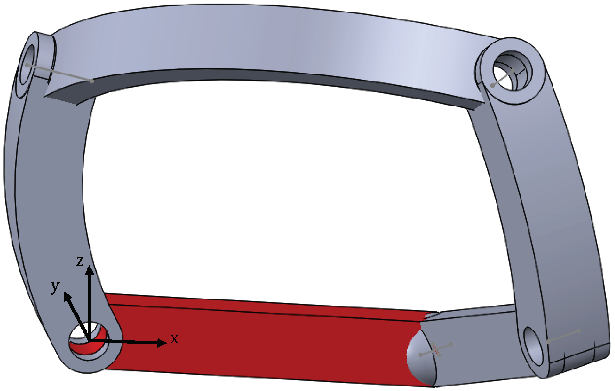
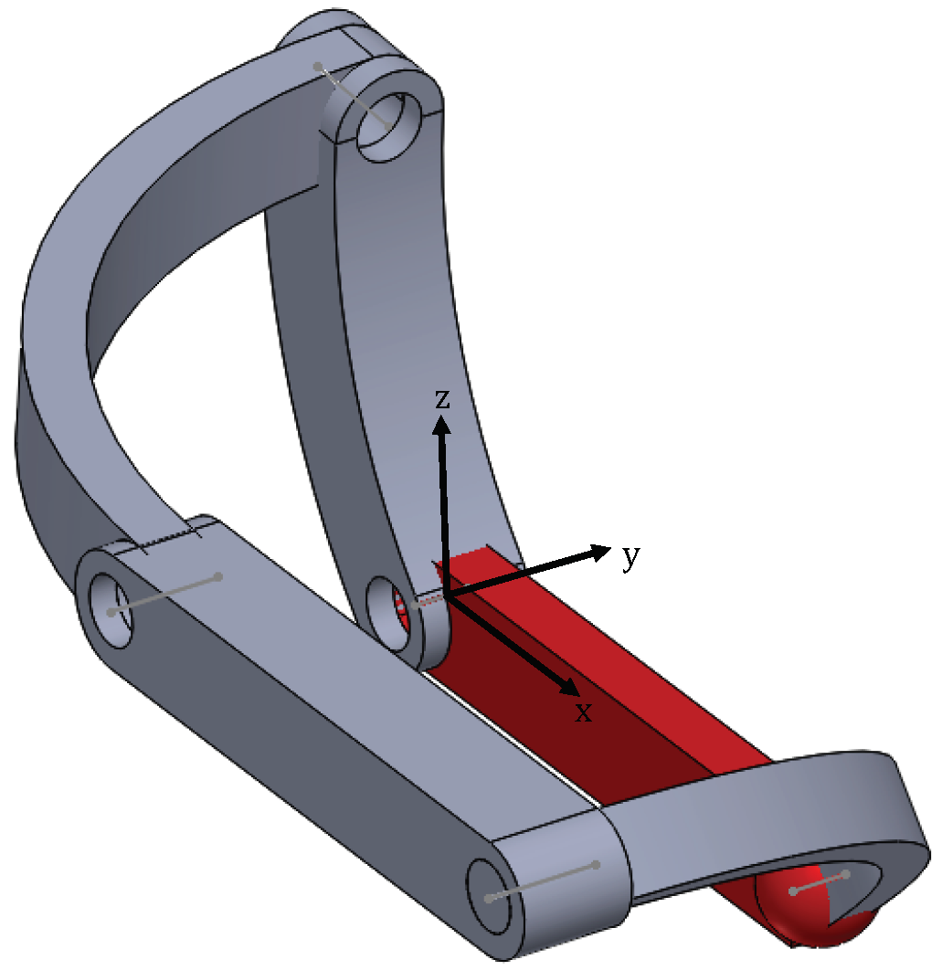
4.1. Perpendicular Architecture

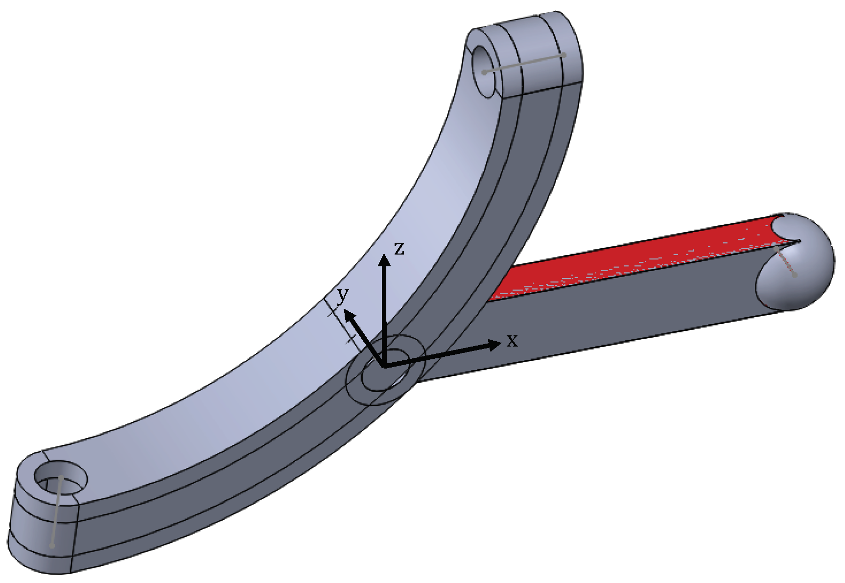
The perpendicular architecture of the mechanism is shown in Figure 2.

In this case we have the D-H link parameters shown in

Table 1. D-H link parameters in the perpendicular architecture.

${\mathit{\alpha }}_{\mathit{i}}$	${\mathit{a}}_{\mathit{i}}$	${\mathit{d}}_{\mathit{i}}$
$-\pi /2$	$r/\sqrt{2}$	0
$\pi /2$	0	$-r/\sqrt{2}$
$\pi /2$	$r/\sqrt{2}$	$r/\sqrt{2}$
$\pi /2$	$-r$	0

.

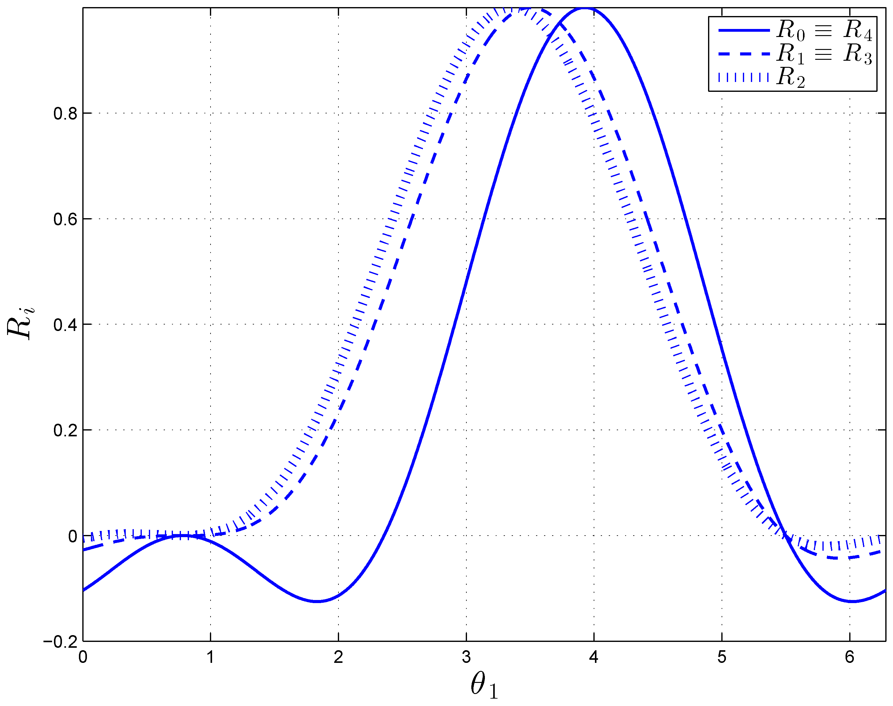
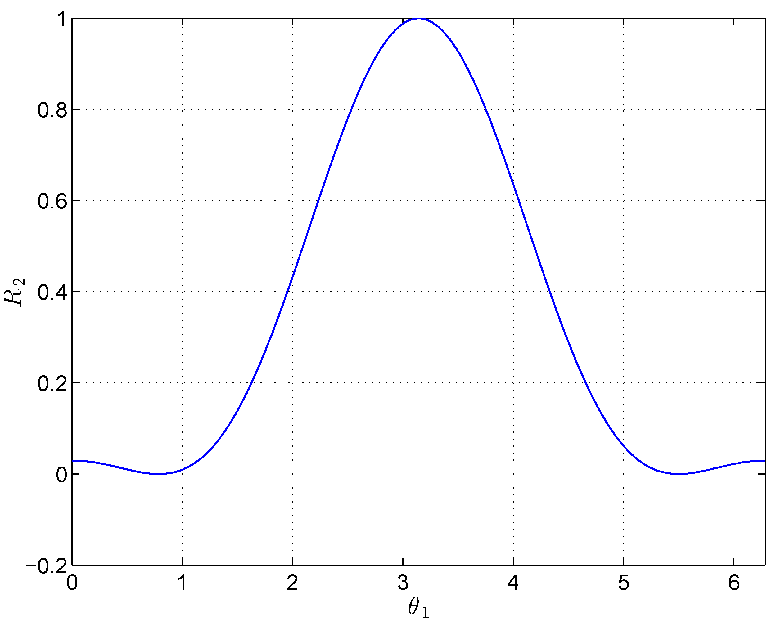
According to Table 1, the spherical joint has the coordinates $x=r$, $y=z=0$ and $\tilde{x}=r(c_{{\theta }_1}-1/\sqrt{2})$, $\tilde{y}=0$ and $\tilde{z}=-r{s}_{{\theta }_1}$, where r is the reference parameter of the mechanism link lengths. Figure 3 shows the values taken by the QME coefficients ${\varphi }_i$’s versus the input angle ${\theta }_1$. In the plot each coefficent is normalized to its maximum such that $R_i={\varphi }_i/\left[max({\varphi }_i)\right]$. It can be seen that all the coefficients vanish for ${\theta }_1=\pm \pi /4$. In these configurations the mechanism has 2 DOF.

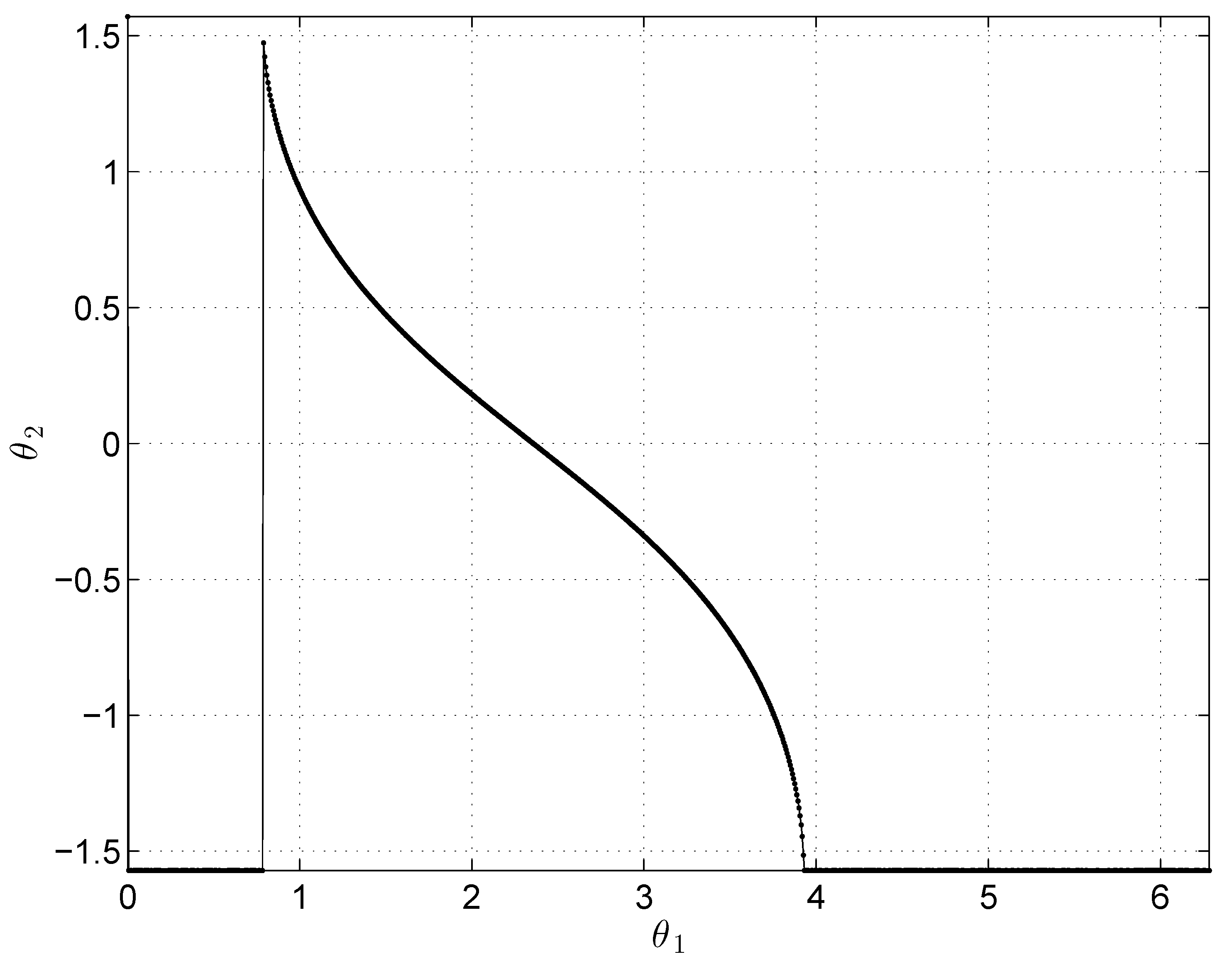
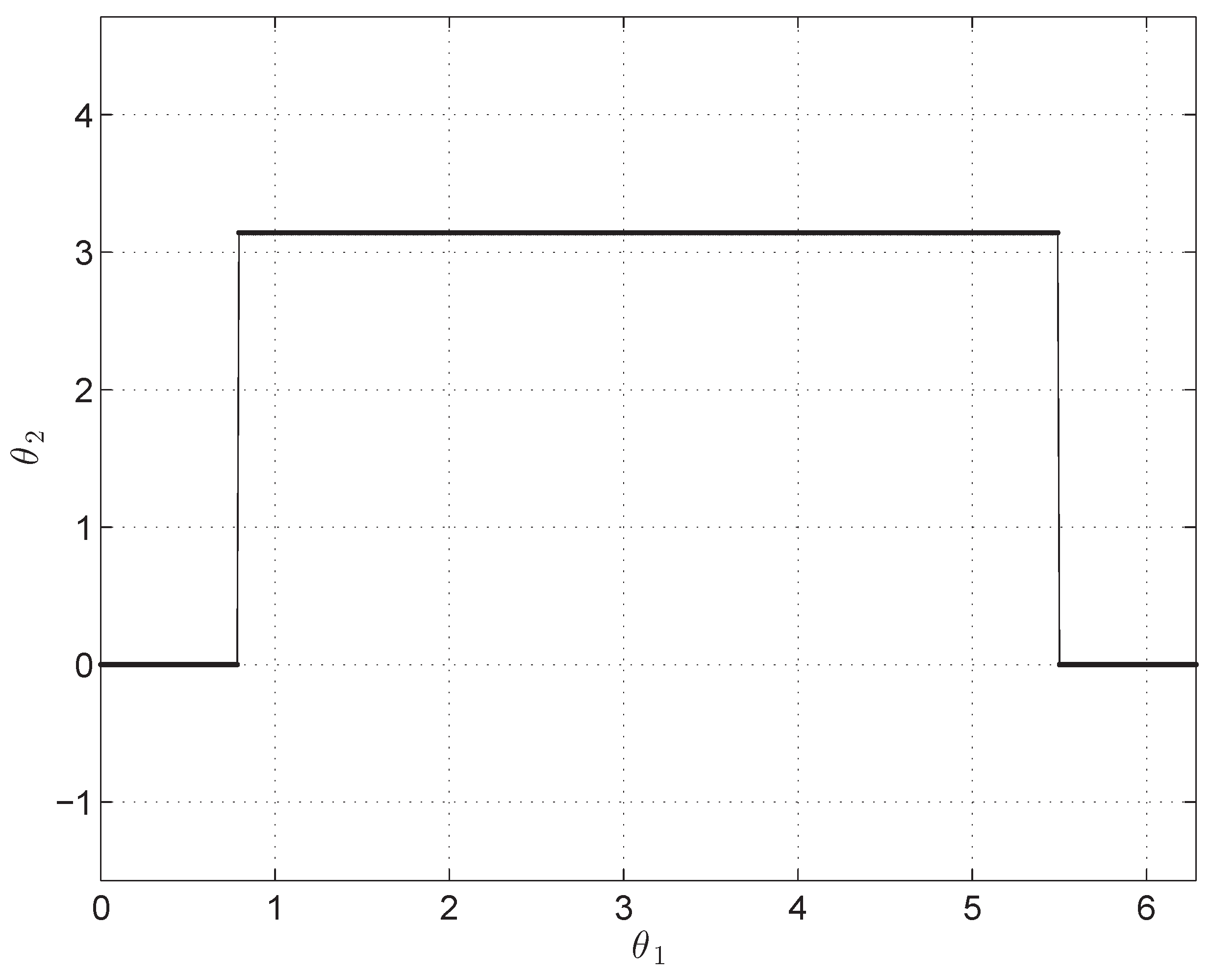
Figure 4 shows the variation of ${\theta }_2$ with the input angle ${\theta }_1$.

As it may be seen the plot can be divided into two branches:

• ${\theta }_1\in [-3/4\pi ,\pi /4)$.
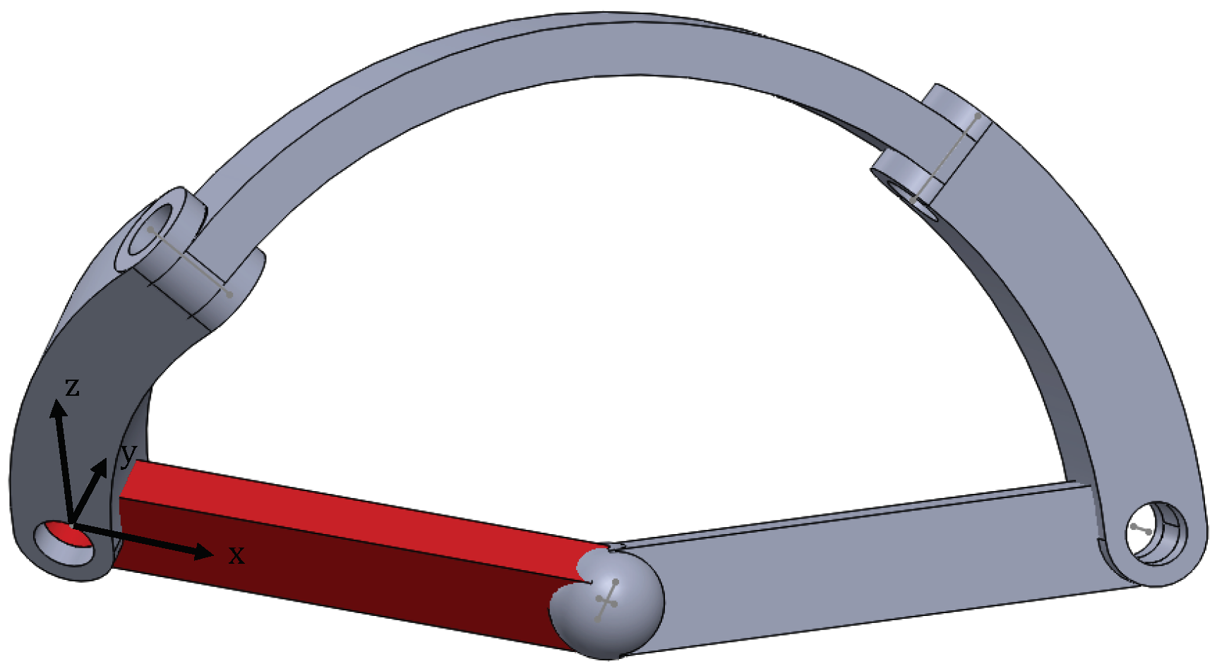
  In this interval ${\theta }_2=-\pi /2$. Indeed, the mechanism is in the folded configuration shown in Figure 5 where the $z_0$- and $z_3$-axes coincide and they are perpendicular to the plane formed by the $z_1$- and $z_2$-axes. The mechanism has 1 DOF being the rotation about the $z_0(z_3)$-axis.
  As mentioned, there are two exceptions due to the fact that the QME coefficients ${\varphi }_i$’s may all vanish as soon as $\tilde{x}=0$. In these configurations the mechanism has 2 DOF, ${\theta }_2$ can take any value whilst ${\theta }_1=\pm \pi /4$ as proved by the first equation of Equation (4). Furthermore, when ${\theta }_1=\pi /4$ point $O_2$ coincides with the sperichal joint S: $\tilde{z}=d_2$ (Figure 6).
• ${\theta }_1\in [\pi /4,5/4\pi )$.
  In this interval the solutions of the QME are real. The mechanism undergoes a smooth 1 DOF motion, (Figure 2). If ${\theta }_1=\pi /4$ then ${\theta }_2⟶\pi /2$ reaching the 2 DOF configuration shown in Figure 6.

In summary, the perpendicular architecture has one 2-DOF motion mode and two 1-DOF motion modes.

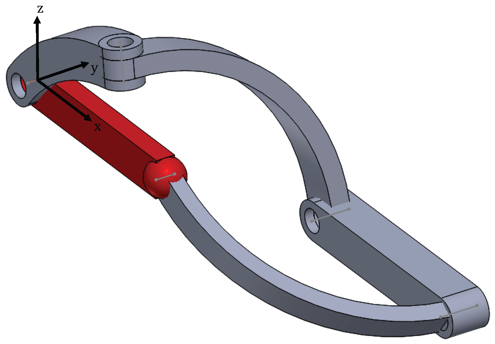
4.2. Parallel Architecture

The parallel architecture of the mechanism is shown in Figure 7.

In this case we have the D-H link parameters shown in

Table 2. D-H link parameters in the parallel architecture.

${\mathit{\alpha }}_{\mathit{i}}$	${\mathit{a}}_{\mathit{i}}$	${\mathit{d}}_{\mathit{i}}$
$-\pi /2$	$r/\sqrt{2}$	0
$\pi /2$	0	$-r/\sqrt{2}$
0	r	r
$-\pi /2$	$-r$	$-r$

.

By inspection of the numerical simulation of the mechanism motion, it is straightforward to find that the QME takes always the form ${\varphi }_2{T}^2=0$ from which ${\theta }_2=2k\pi$, $k\in {\mathbb{Z}}^{+}$. In all these configurations the mechanism undergoes a 1 DOF motion. There are two exceptions due to the fact that ${\varphi }_2$ can vanish as soon as $\tilde{x}=0$. In these configurations the mechanism has 2 DOF, ${\theta }_2$ can take any value whilst ${\theta }_1=\pm \pi /4$ as proved by the first equation of Equation (4) and shown in Figure 8 where $R_2=R_2({\theta }_1)$ with $R_2={\varphi }_2/\left[max({\varphi }_2)\right]$.

It can be noted from Figure 8 the symmetry of the polynomial and therefore of the mechanism motion with respect to the configuration with ${\theta }_1=\pi$. Figure 9 shows the variation of ${\theta }_2$ with the input angle ${\theta }_1$.

Figure 10 and Figure 11 show the mechanism in 1 DOF configuration when approaching the 2 DOF configuration (${\theta }_1⟶\pm \pi /4$) with ${\theta }_2=0$ and ${\theta }_2=\pi$, respectively.

5. Conclusions

The reconfiguration analysis of a single-loop, variable-DOF RRRRS mechanism was carried out. A vector procedure was followed to obtain the quartic motion equation in terms of the joint angle ${\theta }_2$. The equation was written as a polynomial equation according to the half-tangent substitution. The coefficients ${\varphi }_i$’s of the equation depend on the input joint angle ${\theta }_1$ and on the link parameters. The motion of two specific cases of the mechanism has been analyzed. In both cases the mechanism has a 2 DOF motion when $\tilde{x}=\tilde{y}=0$ and $\tilde{z}=\pm r/\sqrt{2}$. In other words when the origin $O_2$ coincides with the spherical joint. These configurations occur when the input angle ${\theta }_1=\pm \pi /4$. It was revealed for the first time that the perpendicular architecture has one 2-DOF motion mode and two 1-DOF motion modes. Despite of the parallel architecture which shows a symmetric ${\theta }_2={\theta }_2({\theta }_1)$ plot, the same plot is unsymmetric in the perpendicular architecture because of the presence of the 1 DOF folded configuration.

References

- Wohlhart, K. Kinematotropic Linkages. In Recent Advances in Robot Kinematics; Lenarcic, J., Parenti-Castelli, V., Eds.; Kluwer Academic: Dordrecht, The Netherlands, 1996; pp. 359–368. [Google Scholar]
- Galletti, C.; Fanghella, P. Single-loop kinematotropic mechanisms. Mech. Mach. Theory 2001, 36, 743–761. [Google Scholar] [CrossRef]
- Fanghella, P.; Galletti, C.; Gianotti, E. Parallel robots that change their group of motion. In Advances in Robot Kinematics; Lenarcic, J., Roth, B., Eds.; Springer: Dordrecht, The Netherlands, 2006; pp. 49–56. [Google Scholar]
- Lee, C.C.; Hervé, J.M. Discontinuously Movable Seven-Link Mechanisms via Group-Algebraic Approach. Proc. Inst. Mech. Eng. Part C 2005, 219, 577–587. [Google Scholar] [CrossRef]
- Kong, X.; Huang, C. Type Synthesis of Single-DOF Single-Loop Mechanisms with Two Operation Modes, Reconfigurable Mechanisms and Robots; KC Edizioni: Genova, Italy, 2009; pp. 141–146. [Google Scholar]
- Wohlhart, K. Multifunctional 7R Linkages. In Proceedings of the International Symposium on Mechanisms and Machine Theory, AzCIFToMM, Izmir, Turkey, 5 October 2010; Volume 8, pp. 85–91. [Google Scholar]
- Lopez-Custodio, P.C.; Rico, J.M.; Cervantes-Sanchez, J.J.; Perez-Soto, G.I. Reconfigurable Mechanisms from the Intersection of Surfaces. ASME J. Mech. Robot. 2016, 8, 021029. [Google Scholar] [CrossRef]
- Zhang, K.; Muller, A.; Dai, J.S. A Novel Reconfigurable 7R Linkage With Multifurcation. In Advances in Reconfigurable Mechanisms and Robots II; Ding, X., Kong, X., Dai, J.S., Eds.; Springer: Cham, Switzerland, 2015; pp. 15–25. [Google Scholar]
- Huang, C.; Kong, X.; Ou, T. Position Analysis of a Bennett-Based Multiple-Mode 7R Linkage. In Proceedings of the ASME 2009 International Design Engineering Technical Conferences and Computers and Information in Engineering Conference, San Diego, CA, USA, 30 August–2 September 2009. ASME Paper No. DETC2009-87241. [Google Scholar]
- He, X.; Kong, X.; Chablat, D.; Caro, S.; Hao, G. Kinematic Analysis of a Single-Loop Reconfigurable 7R Mechanism With Multiple Operation Modes. Robotica 2014, 32, 1171–1188. [Google Scholar] [CrossRef]
- Kong, X.; Pfurner, M. Type Synthesis and Reconfiguration Analysis of a Class of Variable-DOF Single-Loop Mechanisms. Mech. Mach. Theory 2015, 85, 116–128. [Google Scholar] [CrossRef]
- Huang, C.; Tseng, R.; Kong, X. Design and Kinematic Analysis of a Multiple-Mode 5R2P Closed-Loop Linkage. In New Trends in Mechanism Science: Analysis and Design, Mechansims and Machine Science 5; Pisla, D., Ed.; Springer: Dordrecht, The Netherlands, 2010. [Google Scholar]
- Zhang, K.; Dai, J.S. Screw-System-Variation Enabled Reconfiguration of the Bennett Plano-Spherical Hybrid Linkage and its evolved Parallel Mechanism. J. Mech. Des. 2015, 137, 062303. [Google Scholar] [CrossRef]
- He, X.; Kong, X.; Hao, G.; Ritchie, J.M. Design and Analysis of a New 7R Single-Loop Mechanism With 4R, 6R and 7R Operation Modes. In Advances Reconfigurable Mechanisms and Robots II; Ding, X., Kong, X., Dai, J.S., Eds.; Springer: Cham, Switzerland, 2015; pp. 27–37. [Google Scholar]
- Walter, D.R.; Husty, M.L.; Pfurner, M. A complete kinematic analysis of the SNU 3-UPU parallel manipulator, Contemporary Mathematics. Am. Math. Soc. 2009, 496, 331–346. [Google Scholar]
- Kong, X. Reconfiguration analysis of a 3-DOF parallel mechanism using Euler parameter quaternions and algebraic geometry method. Mech. Mach. Theory 2014, 74, 188–201. [Google Scholar] [CrossRef] [Green Version]
- Kong, X.; Yu, J.; Li, D. Reconfiguration Analysis of a Two Degrees-of-Freedom 3-4R Parallel Manipulator with Planar Base and Platform. ASME J. Mech. Robot. 2015, 8, 011019. [Google Scholar] [CrossRef]
- Carbonari, L.; Callegari, M.; Palmieri, G.; Palpacelli, M.C. A new class of reconfigurable parallel kinematic machines. Mech. Mach. Theory 2014, 79, 173–183. [Google Scholar] [CrossRef]
- Nurahmi, L.; Schadlbauer, J.; Caro, S.; Husty, M.; Wenger, P. Kinematic Analysis of the 3-RPS Cube Parallel Manipulator. ASME J. Mech. Rob. 2015, 7, 011008. [Google Scholar] [CrossRef]
- Kong, X. Reconfiguration analysis of a 4-DOF 3-RER parallel manipulator with equilateral triangular base and moving platform. Mech. Mach. Theory 2016, 98, 180–189. [Google Scholar] [CrossRef]
- Kong, X. Reconfiguration Analysis of a Variable Degrees-of-Freedom Parallel Manipulator With Both 3-DOF Planar and 4-DOF 3T1R Operation Modes. In Proceedings of the ASME 2016 International Design Engineering Technical Conferences and Computers and Information in Engineering Conference, Charlotte, NC, USA, 21–24 August 2016. ASME Paper No. DETC2016-59203. [Google Scholar]
- Coste, M.; Demdah, K.M. Extra Modes of Operation and Self Motions in Manipulators Designed for Schoenflies Motion. ASME J. Mech. Robot. 2015, 7, 041020. [Google Scholar] [CrossRef] [Green Version]
- Nurahmi, L.; Caro, S.; Wenger, P.; Schadlbauer, J.; Husty, M. Reconfiguration Analysis of a 4-RUU Parallel Manipulator. Mech. Mach. Theory 2016, 96 (Pt 2), 269–289. [Google Scholar] [CrossRef]
- Arponen, T.; Piipponen, S.; Tuomela, J. Kinematical Analysis of Wunderlich Mechanism. Mech. Mach. Theory 2013, 70, 16–31. [Google Scholar] [CrossRef]
- Pfurner, M.; Kong, X. Algebraic analysis of a new variable-DOF 7R mechanism. In New Trends in Mechanism and Machine Science, Theory and Industrial Applications; Wenger, P., Flores, P., Eds.; Springer: Berlin, Germany, 2016; pp. 71–79. [Google Scholar]
- Kong, X. Reconfiguration analysis of multimode single-loop spatial mechanisms using dual quaternions. J. Mech. Robot. ASME 2017, 9, 051002. [Google Scholar] [CrossRef]
- Kong, X. A variable-DOF single-loop 7R spatial mechanism with five motion modes. Mech. Mach. Theory 2018, 120, 239–249. [Google Scholar] [CrossRef]
- Angeles, J. Fundamental of Robotic Mechanical Systems, 3rd ed.; Springer: Berlin, Germany, 2007. [Google Scholar]
Figure 1.
The RRRRS single-loop mechanism.
Figure 2.
Perpendicular architecture: 1 DOF configuration.
Figure 3.
Perpendicular architecture: vs plot.
Figure 4.
Figure 5.
Perpendicular architecture: folded configuration, 1 DOF.
Figure 6.
Perpendicular architecture: 2 DOF configuration.
Figure 7.
Parallel architecture: 2 DOF configuration.
Figure 8.
Parallel architecture: vs plot.
Figure 9.
Figure 10.
Parallel architecture: 1 DOF configuration with .
Figure 11.