Spacecraft Robot Kinematics Using Dual Quaternions

Abstract

In recent years, there has been a growing interest in servicing orbiting satellites. In most cases, in-orbit servicing relies on the use of spacecraft-mounted robotic manipulators to carry out complicated mission objectives. Dual quaternions, a mathematical tool to conveniently represent pose, has recently been adopted within the space industry to tackle complex control problems during the stages of proximity operations and rendezvous, as well as for the dynamic modeling of robotic arms mounted on a spacecraft. The objective of this paper is to bridge the gap in the use of dual quaternions that exists between the fields of spacecraft control and fixed-base robotic manipulation. In particular, we will cast commonly used tools in the field of robotics as dual quaternion expressions, such as the Denavit-Hartenberg parameterization, or the product of exponentials formula. Additionally, we provide, via examples, a study of the kinematics of different serial manipulator configurations, building up to the case of a completely free-floating robotic system. We provide expressions for the dual velocities of the different types of joints that commonly arise in industrial robots, and we end by providing a collection of results that cast convex constraints commonly encountered by space robots during proximity operations in terms of dual quaternions.

1. Introduction

Robots are increasingly present in our daily lives, with their many uses ranging from simple vacuuming devices to complex manufacturing robotic arms. This growth is sustained by the continuous development of faster and better software and hardware, as well as strong theoretical advances in the areas of kinematics, dynamics, computer vision, sensing, etc. The space industry, owing to obvious reasons having to do with the unfriendliness of the space environment to humans, relies heavily on the use of robotics systems. In fact, interplanetary robotic exploration is at the core of NASA’s Jet Propulsion Laboratory, and a wide variety of companies and governmental agencies are currently developing space-rated robotic manipulation systems for on-orbit satellite servicing [1,2].

The field of robotics is a well-established one. Lately, in the field of fixed-base robotics, progress in the area of kinematics and dynamics has mainly focused on ease of use, and speed and performance improvements [3,4]. The combination between the study of robots and their use in space, i.e., space robotics, must find common ground between the techniques used in both. For example, quaternions are the representation of choice when it comes to attitude parameterization for spacecraft control and estimation, while $\mathrm{SE}\left(2\right)/\mathrm{SE}\left(3\right)$ and the Spatial Vector Algebra [5] are the dominant tools of choice in the fixed-base robotic community. Therefore, with the recent advent of dual quaternions, it is only natural to explore the use of a pose (i.e., position and attitude) representation tool for spacecraft control and estimation in order to study robotic systems mounted on a spacecraft.

Dual quaternion algebra is an extension of the well-known quaternion algebra. The former is used to study rigid body pose while the latter is used extensively to study just the attitude of a rigid body. Dual quaternions have recently seen a proliferation in their use for spacecraft control [6,7,8,9]. Several factors have contributed to the recent interest in dual quaternions in spacecraft control. First, the similarities between quaternion and dual quaternion-based spacecraft controllers and estimators [10] make dual quaternions an appealing tool for the practitioner who is familiar with the (standard) quaternion algebra. Next, dual quaternions naturally encode position information, thus avoiding the artificial separation of rotational and translational motion during control, which becomes essential during proximity operations or robotic servicing missions. More recently, dual quaternions have been used extensively for the dynamic modeling of ground-based robotic manipulators, providing an even stronger argument towards their use for dynamic modeling of spacecraft-mounted robotic manipulators [11].

While dual quaternions have been used for serial robot kinematic design [12,13,14], and for kinematic manipulation of points, vectors, lines, screws and planes [15], few references incorporate velocity information into their study of kinematics. Leclercq et al. [16] studied robot kinematics in the context of human motion using dual quaternions, yielding one of the most complete references to study kinematic chains with dual quaternions. More recently, Quiroz-Omaña and Adorno [17] have made use of dual quaternions in the context of robotic manipulation on a non-holonomic base. The methodologies exhibited in [16,17], however, do not take advantage of the well-known and convenient dual quaternion expression for kinematics, which could avoid manually taking time derivatives of pose expressions. A possible reason for this is the lack of a systematic manner to represent the combined linear and angular velocities of joints in dual algebra, and instead relying on the explicit derivative of pose-like expressions.

Works in the fields of dynamics and spacecraft control have settled on an understanding of the construction of dual velocities [18,19], which can be extended to provide generic expressions for the dual velocities of rigid bodies, or even of the different types of joints that may appear in a serial kinematic chain. In fact, Özgür and Mezouar [20] make use of said representation of dual velocity, commonly given by an expression of the form $\mathit{\omega }=\omega +ϵv$, to perform kinematic control on a robotic arm, yielding a clever representation of the Jacobian matrix that uses dual quaternion screws. Their approach, however, has a fixed base and requires the use of base-frame coordinates—as opposed to body-frame coordinates, which are commonly used in the study of spacecraft motion—to describe the Plücker lines associated to the different joints of the system.

Given the significant interest that dual quaternions have garnered in the last decade in the realm of space applications, it is pertinent to contribute to the literature a straightforward treatment of kinematics with an emphasis on space-based robotic operations. In this paper, we aim to extend the study of robot kinematics using dual quaternions, mainly by lifting the condition that the robotic base must be fixed, allowing it instead to move freely in the three-dimensional space. Additionally, we consider the possibility of incorporating different types of joints, and provide the formulas for the dual velocity of each different type of joint. Along the way, we provide some important well-known results, such as the derivation of the famous quaternion kinematic law, and the aforementioned dual quaternion equivalent, as well as a collection of results that capture convex constraints using dual quaternions. While the latter expressions have been used in the field of Entry, Descent, and Landing (EDL), their incorporation in robotic manipulation for in-orbit servicing missions is also extremely beneficial in order to ensure safety and robustness.

This paper is structured as follows: Section 2 provides the mathematical tools necessary to use quaternion and dual quaternion algebras. Section 3 provides an overview of the most common kinematic tools in the robotics fields in dual quaternion form. Section 4 provides the development of the kinematic equations of motion using dual quaternions, and in Section 5 we provide a brief summary of some important constraint expressions for robotic manipulation cast using dual quaternions. Such constraints arise naturally in many in-orbit servicing missions. Addressing these constraints in a numerically efficient manner (e.g., casting them as convex constraints) leads to safe and elegant solutions of the in-orbit servicing problem.

2. Mathematical Preliminaries

In this section we give an introduction to quaternion and dual quaternion algebras, which provide convenient mathematical frameworks for attitude and pose representations respectively. Next, we provide the theoretical foundations required to study the kinematics of rigid bodies, and in particular how they pertain to serial manipulators.

2.1. Quaternions

The group of quaternions, as defined by Hamilton in 1843, extends the well-known imaginary unit j, which satisfies $j^2=-1$. This non-abelian group is defined by ${\mathbb{Q}}_8\triangleq \{-1,i,j,k:i^2=j^2=k^2=ijk=-1\}$. The algebra constructed from ${\mathbb{Q}}_8$ over the field of real numbers is the quaternion algebra defined as $\mathbb{H}\triangleq \{q=q_0+q_{1}i+q_{2}j+q_{3}k:i^2=j^2=k^2=ijk=-1,q_0,q_1,q_2,q_3\in \mathbb{R}\}$. This defines an associative, non-commutative, division algebra.

In practice, quaternions are often referred to by their scalar and vectors parts as $q=(q_0,\overline{q})$, where $q_0\in \mathbb{R}$ and $\overline{q}={[q_1,q_2,q_3]}^{\mathrm{T}}\in {\mathbb{R}}^3$. The properties of the quaternion algebra are summarized in

Table 1. Quaternion Operations.

Operation	Definition
Addition	$a+b=(a_0+b_0,\overline{a}+\overline{b})$
Scalar multiplication	$\lambda a=(\lambda a_0,\lambda a)$
Multiplication	$ab=(a_0{b}_0-\overline{a}·\overline{b},a_0\overline{b}+b_0\overline{a}+\overline{a}\times \overline{b})$
Conjugate	$a^{*}=(a_0,-\overline{a})$
Dot product	$a·b=(a_0{b}_0+\overline{a}·\overline{b},0_{3\times 1})=\frac{1}{2}(a^{*}b+b^{*}a)$
Cross product	$a\times b=(0,a_0\overline{b}+b_0\overline{a}+\overline{a}\times \overline{b})=\frac{1}{2}(ab-b^{*}{a}^{*})$
Norm	$\parallel a\parallel =\sqrt{a·a}$
Scalar part	$\mathrm{sc}\left(a\right)=(a_0,0_{3\times 1})$
Vector part	$\mathrm{vec}\left(a\right)=(0,\overline{a})$

. Filipe and Tsiotras [7] also conveniently define a multiplication between real 4-by-4 matrices and quaternions, denoted by the ∗ operator, which resembles the well-known matrix-vector multiplication by simply representing the quaternion coefficients as a vector in ${\mathbb{R}}^4$. In other words, given $a=(a_0,\overline{a})\in \mathbb{H}$ and a matrix $M\in {\mathbb{R}}^{4\times 4}$ defined as

$$M=\left[\begin{array}{cc}{M}_{11}& M_{12}\\ M_{21}& M_{22}\end{array}\right],$$

(1)

where $M_{11}\in \mathbb{R},M_{12}\in {\mathbb{R}}^{1\times 3},M_{21}\in {\mathbb{R}}^{3\times 1}$ and $M_{22}\in {\mathbb{R}}^{3\times 3}$, then

$$M\ast a\triangleq (M_{11}{a}_0+M_{12}\overline{a},M_{21}{a}_0+M_{22}\overline{a})\in \mathbb{H}.$$

(2)

Since any rotation can be described by three parameters, the unit norm constraint is imposed on quaternions for attitude representation. Unit quaternions are closed under multiplication, but not under addition. A quaternion describing the orientation of frame $\mathrm{X}$ with respect to frame $\mathrm{Y}$, denoted by $q_{\mathrm{X}/\mathrm{Y}}$, satisfies $q_{\mathrm{X}/\mathrm{Y}}^{*}{q}_{\mathrm{X}/\mathrm{Y}}=q_{\mathrm{X}/\mathrm{Y}}{q}_{\mathrm{X}/\mathrm{Y}}^{*}=\mathtt{1}$, where $\mathtt{1}\triangleq (1,{\overline{0}}_{3\times 1})$. This quaternion can be constructed as $q_{\mathrm{X}/\mathrm{Y}}=(cos(\varphi /2),\overline{n}sin(\theta /2))$, where $\overline{n}$ and $\theta$ are the unit Euler axis, and Euler angle of the rotation respectively. It is worth emphasizing that $q_{\mathrm{Y}/\mathrm{X}}^{*}=q_{\mathrm{X}/\mathrm{Y}}$, and that $q_{\mathrm{X}/\mathrm{Y}}$ and $-q_{\mathrm{X}/\mathrm{Y}}$ represent the same rotation. Furthermore, given quaternions $q_{\mathrm{Y}/\mathrm{X}}$ and $q_{\mathrm{Z}/\mathrm{Y}}$, the quaternion describing the rotation from $\mathrm{X}$ to $\mathrm{Z}$ is given by $q_{\mathrm{Z}/\mathrm{X}}=q_{\mathrm{Y}/\mathrm{X}}{q}_{\mathrm{Z}/\mathrm{Y}}$. For completeness purposes, we define $\mathtt{0}\triangleq (0,{\overline{0}}_{3\times 1})$.

Three-dimensional vectors can also be interpreted as special cases of quaternions. Specifically, given ${\overline{s}}^{\mathrm{X}}\in {\mathbb{R}}^3$, the coordinates of a vector expressed in frame $\mathrm{X}$, its quaternion representation is given by $s^{\mathrm{X}}=(0,{\overline{s}}^{\mathrm{X}})\in {\mathbb{H}}^v$, where ${\mathbb{H}}^v$ is the set of vector quaternions defined as ${\mathbb{H}}^v\triangleq \{(q_0,\overline{q})\in \mathbb{H}:q_0=0\}$ (see Reference [19] for further information). The change of the reference frame for a vector quaternion is achieved by the adjoint operation, and is given by $s^{\mathrm{Y}}=q_{\mathrm{Y}/\mathrm{X}}^{*}{s}^{\mathrm{X}}{q}_{\mathrm{Y}/\mathrm{X}}$. Additionally, given $s\in {\mathbb{H}}^v$, we can define the operation ${[·]}^{\times }:{\mathbb{H}}^v\to {\mathbb{R}}^{4\times 4}$ as

$${\left[s\right]}^{\times }=\left[\begin{array}{cc}0& 0_{1\times 3}\\ 0_{3\times 1}& {\left[\overline{s}\right]}^{\times }\end{array}\right],\mathrm{where}{\left[\overline{s}\right]}^{\times }=\left[\begin{array}{ccc}0& -s_3& s_2\\ s_3& 0& -s_1\\ -s_2& s_1& 0\end{array}\right].$$

(3)

For quaternions $a=(a_0,\overline{a})$ and $b=(b_0,\overline{b})$, the left and right quaternion multiplication operators ${⟦·⟧}_{\mathrm{L}},{⟦·⟧}_{\mathrm{R}}:\mathbb{H}\to {\mathbb{R}}^{4\times 4}$ will be defined as

$${⟦a⟧}_{\mathrm{L}}\ast b\triangleq {⟦b⟧}_{\mathrm{R}}\ast a\triangleq ab,$$

(4)

where

$${⟦a⟧}_{\mathrm{L}}=\left[\begin{array}{cccc}{a}_0& -a_1& -a_2& -a_3\\ a_1& a_0& -a_3& a_2\\ a_2& a_3& a_0& -a_1\\ a_3& -a_2& a_1& a_0\end{array}\right]=\left[\begin{array}{cc}{a}_0& -{\overline{a}}^{\mathrm{T}}\\ \overline{a}& a_0{\mathbb{I}}_3+{\left[\overline{a}\right]}^{\times }\end{array}\right],$$

(5)

$${⟦b⟧}_{\mathrm{R}}=\left[\begin{array}{cccc}{b}_0& -b_1& -b_2& -b_3\\ b_1& b_0& b_3& -b_2\\ b_2& -b_3& b_0& b_1\\ b_3& b_2& -b_1& b_0\end{array}\right]=\left[\begin{array}{cc}{b}_0& -{\overline{b}}^{\mathrm{T}}\\ \overline{b}& b_0{\mathbb{I}}_3-{\left[\overline{b}\right]}^{\times }\end{array}\right].$$

(6)

2.2. Dual Quaternions

We define the dual quaternion group as

$$\begin{array}{cc}\hfill {\mathbb{Q}}_d:=\{-1,i,j,k,ϵ,ϵi,ϵj,ϵk:& i^2=j^2=k^2=ijk=-1,\hfill \\ & ϵi=iϵ,ϵj=jϵ,ϵk=kϵ,ϵ\ne 0,{ϵ}^2=0\}.\hfill \end{array}$$

(7)

The dual quaternion algebra arises as the algebra of the dual quaternion group ${\mathbb{Q}}_d$ over the field of real numbers, and is denoted as ${\mathbb{H}}_d$. When dealing with the modeling of mechanical systems, it is convenient to present this algebra as ${\mathbb{H}}_d=\{\mathit{q}=q_r+ϵq_d:q_r,q_d\in \mathbb{H}\}$, where $ϵ$ is the dual unit. We call $q_r$ the real part, and $q_d$ the dual part of the dual quaternion $\mathit{q}$.

Filipe and Tsiotras [7,8,19,21] have laid out much of the groundwork in terms of the notation and basic properties of dual quaternions for spacecraft problems. The main properties of the dual quaternion algebra are listed in

Table 2. Dual Quaternion Operations.

Operation	Definition
Addition	$\mathit{a}+\mathit{b}=(a_r+b_r)+ϵ(a_d+b_d)$
Scalar multiplication	$\lambda \mathit{a}=\left(\lambda a_r\right)+ϵ\left(\lambda a_d\right)$
Multiplication	$\mathit{a}\mathit{b}=\left(a_r{b}_r\right)+ϵ(a_d{b}_r+a_r{b}_d)$
Conjugate	${\mathit{a}}^{*}=\left(a_r^{*}\right)+ϵ\left(a_d^{*}\right)$
Dot product	$\mathit{a}·\mathit{b}=(a_r·b_r)+ϵ(a_d·b_r+a_r·b_d)=\frac{1}{2}({\mathit{a}}^{*}\mathit{b}+{\mathit{b}}^{*}\mathit{a})$
Cross product	$\mathit{a}\times \mathit{b}=(a_r\times b_r)+ϵ(a_d\times b_r+a_r\times b_d)=\frac{1}{2}(\mathit{a}\mathit{b}-{\mathit{b}}^{*}{\mathit{a}}^{*})$
Circle product	$\mathit{a}\circ \mathit{b}=(a_r·b_r+a_d·b_d)+ϵ\mathtt{0}$
Swap	${\mathit{a}}^{\mathsf{s}}=a_d+ϵa_r$
Norm	$\parallel a\parallel =\sqrt{a\circ a}$
Scalar part	$\mathrm{sc}\left(\mathit{a}\right)=\mathrm{sc}\left(a_r\right)+ϵ\mathrm{sc}\left(a_d\right)$
Vector part	$\mathrm{vec}\left(\mathit{a}\right)=\mathrm{vec}\left(a_r\right)+ϵ\mathrm{vec}\left(a_d\right)$

. Filipe and Tsiotras [7] also conveniently define a multiplication between matrices and dual quaternions, denoted by the ⋆ operator, that resembles the well-known real matrix-vector multiplication by simply representing the dual quaternion coefficients as a vector in ${\mathbb{R}}^8$. In other words, given $\mathit{a}=a_r+ϵa_d\in {\mathbb{H}}_d$ and a matrix $\mathit{M}\in {\mathbb{R}}^{8\times 8}$ defined as

$$\mathit{M}=\left[\begin{array}{cc}{M}_{11}& M_{12}\\ M_{21}& M_{22}\end{array}\right],$$

(8)

where $M_{11},M_{12},M_{21},M_{22}\in {\mathbb{R}}^{4\times 4}$, then

$$\mathit{M}\star \mathit{a}\triangleq (M_{11}\ast a_r+M_{12}\ast a_d)+ϵ(M_{21}\ast a_r+M_{22}\ast a_d)\in {\mathbb{H}}_d.$$

(9)

Analogous to the set of vector quaternions ${\mathbb{H}}^v$, we can define the set of vector dual quaternions as ${\mathbb{H}}_d^v\triangleq \{\mathit{q}=q_r+ϵq_d:q_r,q_d\in {\mathbb{H}}^v\}$. For vector dual quaternions we will define the skew-symmetric operator ${[·]}^{\times }:{\mathbb{H}}_d^v\to {\mathbb{R}}^{8\times 8}$,

$${\left[\mathit{s}\right]}^{\times }=\left[\begin{array}{cc}{\left[s_r\right]}^{\times }& 0_{4\times 4}\\ {\left[s_d\right]}^{\times }& {\left[s_r\right]}^{\times }\end{array}\right].$$

(10)

For dual quaternions $\mathit{a}=a_r+ϵa_d$ and $\mathit{b}=b_r+ϵb_d\in {\mathbb{H}}_d$, the left and right dual quaternion multiplication operators $⟦\phantom{·}·{\phantom{·}⟧}_{\mathrm{L}},⟦\phantom{·}·{\phantom{·}⟧}_{\mathrm{R}}:{\mathbb{H}}_d\to {\mathbb{R}}^{8\times 8}$ are defined as

$$\mathit{a}\mathit{b}\triangleq ⟦\phantom{\mathit{a}}\mathit{a}{\phantom{\mathit{a}}⟧}_{\mathrm{L}}\star \mathit{b}\triangleq ⟦\phantom{\mathit{b}}\mathit{b}{\phantom{\mathit{b}}⟧}_{\mathrm{R}}\star \mathit{a},$$

(11)

where

$$⟦\phantom{\mathit{a}}\mathit{a}{\phantom{\mathit{a}}⟧}_{\mathrm{L}}=\left[\begin{array}{cc}{⟦a_r⟧}_{\mathrm{L}}& 0_{4\times 4}\\ {⟦a_d⟧}_{\mathrm{L}}& {⟦a_r⟧}_{\mathrm{L}}\end{array}\right]\mathrm{and}⟦\phantom{\mathit{b}}\mathit{b}{\phantom{\mathit{b}}⟧}_{\mathrm{R}}=\left[\begin{array}{cc}{⟦b_r⟧}_{\mathrm{R}}& 0_{4\times 4}\\ {⟦b_d⟧}_{\mathrm{R}}& {⟦b_r⟧}_{\mathrm{R}}\end{array}\right].$$

(12)

Since rigid body motion has six degrees of freedom, a dual quaternion needs two constraints to parameterize it. The dual quaternion describing the relative pose of frame $\mathrm{B}$ relative to frame $\mathrm{I}$ is given by ${\mathit{q}}_{\mathrm{B}/\mathrm{I}}=q_{\mathrm{B}/\mathrm{I},r}+ϵq_{\mathrm{B}/\mathrm{I},d}=q_{\mathrm{B}/\mathrm{I}}+ϵ\frac{1}{2}{q}_{\mathrm{B}/\mathrm{I}}{r}_{\mathrm{B}/\mathrm{I}}^{\mathrm{B}}$, where $r_{\mathrm{B}/\mathrm{I}}^{\mathrm{B}}$ is the position quaternion describing the location of the origin of frame $\mathrm{B}$ relative to that of frame $\mathrm{I}$, expressed in $\mathrm{B}$-frame coordinates. It can be easily observed that $q_{\mathrm{B}/\mathrm{I},r}·q_{\mathrm{B}/\mathrm{I},r}=\mathtt{1}$ and $q_{\mathrm{B}/\mathrm{I},r}·q_{\mathrm{B}/\mathrm{I},d}=\mathtt{0}$, where $\mathtt{0}=(0,\overline{0})$, providing the two necessary constraints. Thus, a dual quaternion representing a pose transformation is a unit dual quaternion, since it satisfies $\mathit{q}·\mathit{q}={\mathit{q}}^{*}\mathit{q}=\mathbf{1}$, where $\mathbf{1}\triangleq \mathtt{1}+ϵ\mathtt{0}$. Additionally, we also define $\mathbf{0}\triangleq \mathtt{0}+ϵ\mathtt{0}$.

Similar to the standard quaternion relationships, the frame transformations laid out in

Table 3. Unit Dual Quaternion Operations.

Composition of transformations	${\mathit{q}}_{\mathrm{Z}/\mathrm{X}}={\mathit{q}}_{\mathrm{Y}/\mathrm{X}}{\mathit{q}}_{\mathrm{Z}/\mathrm{Y}}$
Inverse, Conjugate	${\mathit{q}}_{\mathrm{Y}/\mathrm{X}}^{*}={\mathit{q}}_{\mathrm{X}/\mathrm{Y}}$

can be easily verified.

In Reference [19] it was proven that for a dual unit quaternion $\mathit{q}\in {\mathbb{H}}_d$, $\mathit{q}$ and $-\mathit{q}$ represent the same frame transformation, property inherited from the space of quaternions. Therefore, as is done in practice for quaternions, dual quaternions can be subjected to properization, which is the action of redefining a dual quaternion so that the scalar part of the quaternion is always positive. Formally, we can define the properization of a dual quaternion $\mathit{q}=q_r+ϵq_d$ as

$$\mathit{q}:=-\mathit{q}\mathrm{if}{\left(q_r\right)}_0<0,$$

(13)

where ${\left(q_r\right)}_0$ is the scalar part of $q_r$. Just like in the case of quaternions, dual quaternions also inherit the so-called unwinding phenomenon, first described in [22], which is most important in control applications.

A useful equation is the generalization of the velocity of a rigid body in dual form, which contains both the linear and angular velocity components. The dual velocity of the $\mathrm{Y}$-frame with respect to the $\mathrm{Z}$-frame, expressed in $\mathrm{X}$-frame coordinates, is defined as

$${\mathit{\omega }}_{\mathrm{Y}/\mathrm{Z}}^{\mathrm{X}}={\mathit{q}}_{\mathrm{X}/\mathrm{Y}}^{*}{\mathit{\omega }}_{\mathrm{Y}/\mathrm{Z}}^{\mathrm{Y}}{\mathit{q}}_{\mathrm{X}/\mathrm{Y}}={\omega }_{\mathrm{Y}/\mathrm{Z}}^{\mathrm{X}}+ϵ(v_{\mathrm{Y}/\mathrm{Z}}^{\mathrm{X}}+{\omega }_{\mathrm{Y}/\mathrm{Z}}^{\mathrm{X}}\times r_{\mathrm{X}/\mathrm{Y}}^{\mathrm{X}}),$$

(14)

where ${\omega }_{\mathrm{Y}/\mathrm{Z}}^{\mathrm{X}}=(0,{\overline{\omega }}_{\mathrm{Y}/\mathrm{Z}}^{\mathrm{X}})$ and $v_{\mathrm{Y}/\mathrm{Z}}^{\mathrm{X}}=(0,{\overline{v}}_{\mathrm{Y}/\mathrm{Z}}^{\mathrm{X}})$, ${\overline{\omega }}_{\mathrm{Y}/\mathrm{Z}}^{\mathrm{X}}$ and ${\overline{v}}_{\mathrm{Y}/\mathrm{Z}}^{\mathrm{X}}\in {\mathbb{R}}^3$ are respectively the angular and linear velocity of the $\mathrm{Y}$-frame with respect to the $\mathrm{Z}$-frame expressed in $\mathrm{X}$-frame coordinates, and $r_{\mathrm{X}/\mathrm{Y}}^{\mathrm{X}}=(0,{\overline{r}}_{\mathrm{X}/\mathrm{Y}}^{\mathrm{X}})$, where ${\overline{r}}_{\mathrm{X}/\mathrm{Y}}^{\mathrm{X}}\in {\mathbb{R}}^3$ is the position vector from the origin of the $\mathrm{Y}$-frame to the origin of the $\mathrm{X}$-frame expressed in $\mathrm{X}$-frame coordinates. In particular, from Equation (14) we observe that the dual velocity of a rigid body assigned to frame $\mathrm{B}$ with respect to an inertial frame $\mathrm{I}$, expressed in $\mathrm{B}$-frame coordinates is given as ${\mathit{\omega }}_{\mathrm{B}/\mathrm{I}}^{\mathrm{B}}={\omega }_{\mathrm{B}/\mathrm{I}}^{\mathrm{B}}+ϵv_{\mathrm{B}/\mathrm{I}}^{\mathrm{B}}$. However, if we wanted to express this same dual velocity in inertial frame coordinates, as per Equation (14) we would get ${\mathit{\omega }}_{\mathrm{B}/\mathrm{I}}^{\mathrm{I}}={\omega }_{\mathrm{B}/\mathrm{I}}^{\mathrm{I}}+ϵ(v_{\mathrm{B}/\mathrm{I}}^{\mathrm{I}}+{\omega }_{\mathrm{B}/\mathrm{I}}^{\mathrm{I}}\times r_{\mathrm{I}/\mathrm{B}}^{\mathrm{I}})$. We will formally introduce frame transformations next.

2.3. Frame Transformations Using Dual Quaternions

As is common in the study of kinematics, frame transformations are vital for the determination of velocities and accelerations with respect to different frames. A dual velocity, or dual acceleration, can be described by a dual vector quaternion ${\mathit{s}}^{\mathrm{X}}\in {\mathbb{H}}_d^v$ expressed in $\mathrm{X}$-frame coordinates as ${\mathit{s}}^{\mathrm{X}}\triangleq s_r^{\mathrm{X}}+ϵs_d^{\mathrm{X}}$, where $s_r^{\mathrm{X}},s_d^{\mathrm{X}}\in {\mathbb{H}}^v$. As noted for Equation (14), frame transformations are given by the adjoint operation as

$$\begin{array}{cc}\hfill {\mathit{s}}^{\mathrm{Y}}& ={\mathit{q}}_{\mathrm{Y}/\mathrm{X}}^{*}{\mathit{s}}^{\mathrm{X}}{\mathit{q}}_{\mathrm{Y}/\mathrm{X}}\hfill \\ & =(q_{\mathrm{Y}/\mathrm{X}}+ϵ\frac{1}{2}{r}_{\mathrm{Y}/\mathrm{X}}^{\mathrm{X}}{q}_{\mathrm{Y}/\mathrm{X}})*(s_r^{\mathrm{X}}+ϵs_d^{\mathrm{X}})(q_{\mathrm{Y}/\mathrm{X}}+ϵ\frac{1}{2}{r}_{\mathrm{Y}/\mathrm{X}}^{\mathrm{X}}{q}_{\mathrm{Y}/\mathrm{X}})\hfill \\ & =(q_{\mathrm{Y}/\mathrm{X}}^{*}+ϵ\frac{1}{2}{q}_{\mathrm{Y}/\mathrm{X}}^{*}{r}_{\mathrm{Y}/\mathrm{X}}^{\mathrm{X}*})(s_r^{\mathrm{X}}+ϵs_d^{\mathrm{X}})(q_{\mathrm{Y}/\mathrm{X}}+ϵ\frac{1}{2}{r}_{\mathrm{Y}/\mathrm{X}}^{\mathrm{X}}{q}_{\mathrm{Y}/\mathrm{X}})\hfill \\ & =(q_{\mathrm{Y}/\mathrm{X}}^{*}-ϵ\frac{1}{2}{q}_{\mathrm{Y}/\mathrm{X}}^{*}{r}_{\mathrm{Y}/\mathrm{X}}^{\mathrm{X}})(s_r^{\mathrm{X}}+ϵs_d^{\mathrm{X}})(q_{\mathrm{Y}/\mathrm{X}}+ϵ\frac{1}{2}{r}_{\mathrm{Y}/\mathrm{X}}^{\mathrm{X}}{q}_{\mathrm{Y}/\mathrm{X}})\hfill \\ & =(q_{\mathrm{Y}/\mathrm{X}}^{*}-ϵ\frac{1}{2}{q}_{\mathrm{Y}/\mathrm{X}}^{*}{r}_{\mathrm{Y}/\mathrm{X}}^{\mathrm{X}})(s_r^{\mathrm{X}}{q}_{\mathrm{Y}/\mathrm{X}}+ϵ(s_d^{\mathrm{X}}{q}_{\mathrm{Y}/\mathrm{X}}+s_r^{\mathrm{X}}\frac{1}{2}{r}_{\mathrm{Y}/\mathrm{X}}^{\mathrm{X}}{q}_{\mathrm{Y}/\mathrm{X}}))\hfill \\ & =q_{\mathrm{Y}/\mathrm{X}}^{*}{s}_r^{\mathrm{X}}{q}_{\mathrm{Y}/\mathrm{X}}-ϵ(\frac{1}{2}{q}_{\mathrm{Y}/\mathrm{X}}^{*}{r}_{\mathrm{Y}/\mathrm{X}}^{\mathrm{X}}{s}_r^{\mathrm{X}}{q}_{\mathrm{Y}/\mathrm{X}})+ϵ(q_{\mathrm{Y}/\mathrm{X}}^{*}{s}_d^{\mathrm{X}}{q}_{\mathrm{Y}/\mathrm{X}}+q_{\mathrm{Y}/\mathrm{X}}^{*}{s}_r^{\mathrm{X}}\frac{1}{2}{r}_{\mathrm{Y}/\mathrm{X}}^{\mathrm{X}}{q}_{\mathrm{Y}/\mathrm{X}})\hfill \\ & =s_r^{\mathrm{Y}}+ϵ(s_d^{\mathrm{Y}}+\frac{1}{2}{q}_{\mathrm{Y}/\mathrm{X}}^{*}{s}_r^{\mathrm{X}}{q}_{\mathrm{Y}/\mathrm{X}}{q}_{\mathrm{Y}/\mathrm{X}}^{*}{r}_{\mathrm{Y}/\mathrm{X}}^{\mathrm{X}}{q}_{\mathrm{Y}/\mathrm{X}}-\frac{1}{2}{q}_{\mathrm{Y}/\mathrm{X}}^{*}{r}_{\mathrm{Y}/\mathrm{X}}^{\mathrm{X}}{q}_{\mathrm{Y}/\mathrm{X}}{q}_{\mathrm{Y}/\mathrm{X}}^{*}{s}_r^{\mathrm{X}}{q}_{\mathrm{Y}/\mathrm{X}})\hfill \\ & =s_r^{\mathrm{Y}}+ϵ(s_d^{\mathrm{Y}}+\frac{1}{2}{s}_r^{\mathrm{Y}}{r}_{\mathrm{Y}/\mathrm{X}}^{\mathrm{Y}}-\frac{1}{2}{r}_{\mathrm{Y}/\mathrm{X}}^{\mathrm{Y}}{s}_r^{\mathrm{Y}})\hfill \\ & =s_r^{\mathrm{Y}}+ϵ(s_d^{\mathrm{Y}}+\frac{1}{2}{s}_r^{\mathrm{Y}}{r}_{\mathrm{Y}/\mathrm{X}}^{\mathrm{Y}}-\frac{1}{2}{(r_{\mathrm{Y}/\mathrm{X}}^{\mathrm{Y}})}^{*}{(s_r^{\mathrm{Y}})}^{*}).\hfill \end{array}$$

By the definition of the cross product of two quaternion quantities given in Table 1, we get that

$$\begin{array}{c}\hfill \begin{array}{cc}\hfill {\mathit{s}}^{\mathrm{Y}}& ={\mathit{q}}_{\mathrm{Y}/\mathrm{X}}^{*}{\mathit{s}}^{\mathrm{X}}{\mathit{q}}_{\mathrm{Y}/\mathrm{X}}\hfill \\ & =s_r^{\mathrm{Y}}+ϵ(s_d^{\mathrm{Y}}+s_r^{\mathrm{Y}}\times r_{\mathrm{Y}/\mathrm{X}}^{\mathrm{Y}})\hfill \\ & =s_r^{\mathrm{Y}}+ϵ(s_d^{\mathrm{Y}}+r_{\mathrm{X}/\mathrm{Y}}^{\mathrm{Y}}\times s_r^{\mathrm{Y}}).\hfill \end{array}\end{array}$$

(15)

Analogously, the transformation of a dual vector ${\mathit{s}}^{\mathrm{Y}}\triangleq s_r^{\mathrm{Y}}+ϵs_d^{\mathrm{Y}}$ can be easily derived using the procedure described above to be:

$$\begin{array}{c}\hfill \begin{array}{cc}\hfill {\mathit{s}}^{\mathrm{X}}& ={\mathit{q}}_{\mathrm{Y}/\mathrm{X}}{\mathit{s}}^{\mathrm{Y}}{\mathit{q}}_{\mathrm{Y}/\mathrm{X}}^{*}\hfill \\ & =s_r^{\mathrm{X}}+ϵ(s_d^{\mathrm{X}}+s_r^{\mathrm{X}}\times r_{\mathrm{X}/\mathrm{Y}}^{\mathrm{X}})\hfill \\ & =s_r^{\mathrm{X}}+ϵ(s_d^{\mathrm{X}}+r_{\mathrm{Y}/\mathrm{X}}^{\mathrm{X}}\times s_r^{\mathrm{X}}).\hfill \end{array}\end{array}$$

(16)

As is standard notation, we can define the group adjoint operation for unit dual quaternions as

$${\mathrm{Ad}}_{\mathit{q}}\mathit{s}\triangleq \mathit{q}\mathit{s}{\mathit{q}}^{-1}=\mathit{q}\mathit{s}{\mathit{q}}^{*}.$$

(17)

Therefore, using this notation, the frame transformations derived above can be cast as

$$\begin{array}{cc}\hfill {\mathit{s}}^{\mathrm{X}}& ={\mathrm{Ad}}_{{\mathit{q}}_{\mathrm{Y}/\mathrm{X}}}{\mathit{s}}^{\mathrm{Y}}\hfill \end{array}$$

(18)

$$\begin{array}{cc}\hfill {\mathit{s}}^{\mathrm{Y}}& ={\mathrm{Ad}}_{{\mathit{q}}_{\mathrm{Y}/\mathrm{X}}^{*}}{\mathit{s}}^{\mathrm{X}}={\mathrm{Ad}}_{{\mathit{q}}_{\mathrm{X}/\mathrm{Y}}}{\mathit{s}}^{\mathrm{X}}\hfill \end{array}$$

(19)

The power of dual quaternions goes beyond the ability to represent pose and transform dual velocities and accelerations. In fact, dual quaternions can natively—without constructs that fall outside the algebra—encode the most typical geometric objects such as points, lines and planes. The reader is referred to the literature to find such parameterizations and the correct dual quaternion transformation [15,16].

2.4. Derivation of Fundamental Kinematic Laws

In this section we will derive both the quaternion and dual quaternion kinematic laws. We will make the time dependence explicit only when necessary for clarity.

The three-dimensional attitude kinematics evolve as

$${\dot{q}}_{\mathrm{X}/\mathrm{Y}}=\frac{1}{2}{q}_{\mathrm{X}/\mathrm{Y}}{\omega }_{\mathrm{X}/\mathrm{Y}}^{\mathrm{X}}=\frac{1}{2}{\omega }_{\mathrm{X}/\mathrm{Y}}^{\mathrm{Y}}{q}_{\mathrm{X}/\mathrm{Y}},$$

(20)

where ${\omega }_{\mathrm{X}/\mathrm{Y}}^{\mathrm{Z}}\triangleq (0,{\overline{\omega }}_{\mathrm{X}/\mathrm{Y}}^{\mathrm{Z}})\in {\mathbb{H}}^v$ and ${\overline{\omega }}_{\mathrm{X}/\mathrm{Y}}^{\mathrm{Z}}\in {\mathbb{R}}^3$ is the angular velocity of frame $\mathrm{X}$ with respect to frame $\mathrm{Y}$ expressed in $\mathrm{Z}$-frame coordinates. On the other hand, the dual quaternion kinematics can be expressed as [7]

$${\dot{\mathit{q}}}_{\mathrm{X}/\mathrm{Y}}=\frac{1}{2}{\mathit{q}}_{\mathrm{X}/\mathrm{Y}}{\mathit{\omega }}_{\mathrm{X}/\mathrm{Y}}^{\mathrm{X}}=\frac{1}{2}{\mathit{\omega }}_{\mathrm{X}/\mathrm{Y}}^{\mathrm{Y}}{\mathit{q}}_{\mathrm{X}/\mathrm{Y}}.$$

(21)

Lemma 1.

The attitude of a rigid body evolves as ${\dot{q}}_{\mathrm{X}/\mathrm{Y}}=\frac{1}{2}{q}_{\mathrm{X}/\mathrm{Y}}{\omega }_{\mathrm{X}/\mathrm{Y}}^{\mathrm{X}}$, as stated in Equation (20).

Proof. 

Denote the infinitesimal rotation about axis $\widehat{u}$ by $\Delta \theta$. The quaternion that represents this rotation is constructed as $\delta q_{\mathrm{X}/\mathrm{Y}}(\Delta t)\triangleq \left(cos\left(\Delta \theta /2\right),\widehat{u}sin\left(\Delta \theta /2\right)\right)$. Therefore, $q_{\mathrm{X}/\mathrm{Y}}(t+\Delta t)=q_{\mathrm{X}/\mathrm{Y}}(t)\delta q_{\mathrm{X}/\mathrm{Y}}(\Delta t)$. Then, for a small rotation angle, $\delta q_{\mathrm{X}/\mathrm{Y}}(\Delta t)=\left(1,\widehat{u}\Delta \theta /2\right)$. Substituting into the previous expression for $q_{\mathrm{X}/\mathrm{Y}}(t+\Delta t)$, we obtain

$$\begin{array}{c}\hfill \begin{array}{cc}\hfill q_{\mathrm{X}/\mathrm{Y}}(t+\Delta t)& =q_{\mathrm{X}/\mathrm{Y}}(t)\left(1,\widehat{u}\Delta \theta /2\right)\hfill \\ & =q_{\mathrm{X}/\mathrm{Y}}(t)\left(\mathtt{1}+(0,\widehat{u}\Delta \theta /2)\right)\hfill \\ & =q_{\mathrm{X}/\mathrm{Y}}(t)+\frac{1}{2}{q}_{\mathrm{X}/\mathrm{Y}}(t)\widehat{u}\Delta \theta .\hfill \end{array}\end{array}$$

(22)

Manipulating the expression and dividing by $\Delta t$, we obtain

$$\begin{array}{c}\hfill \begin{array}{c}\hfill \frac{q_{\mathrm{X}/\mathrm{Y}}(t+\Delta t)-q_{\mathrm{X}/\mathrm{Y}}(t)}{\Delta t}=\frac{1}{2}{q}_{\mathrm{X}/\mathrm{Y}}(t)\widehat{u}\frac{\Delta \theta }{\Delta t},\end{array}\end{array}$$

(23)

and invoking the limit as $\Delta t\to 0$ yields

$$\begin{array}{c}\hfill \begin{array}{c}\hfill {\dot{q}}_{\mathrm{X}/\mathrm{Y}}(t)=\frac{1}{2}{q}_{\mathrm{X}/\mathrm{Y}}(t){\omega }_{\mathrm{X}/\mathrm{Y}}^{\mathrm{X}}(t),\end{array}\end{array}$$

(24)

where we have defined the angular velocity as ${\omega }_{\mathrm{X}/\mathrm{Y}}^{\mathrm{X}}\triangleq \widehat{u}\dot{\theta }$, i.e., the rate of rotation about the instantaneous Euler axis. ☐

Lemma 2.

The pose of a rigid body evolves as ${\dot{\mathit{q}}}_{\mathrm{X}/\mathrm{Y}}=\frac{1}{2}{\mathit{q}}_{\mathrm{X}/\mathrm{Y}}{\mathit{\omega }}_{\mathrm{X}/\mathrm{Y}}^{\mathrm{X}}$, as stated in Equation (21).

Proof. 

Taking the derivative of ${\mathit{q}}_{\mathrm{X}/\mathrm{Y}}=q_{\mathrm{X}/\mathrm{Y}}+ϵ\frac{1}{2}{q}_{\mathrm{X}/\mathrm{Y}}{r}_{\mathrm{X}/\mathrm{Y}}^{\mathrm{X}}$ we get

$$\begin{array}{cc}\hfill {\dot{\mathit{q}}}_{\mathrm{X}/\mathrm{Y}}& ={\dot{q}}_{\mathrm{X}/\mathrm{Y}}+ϵ(\frac{1}{2}{\dot{q}}_{\mathrm{X}/\mathrm{Y}}{r}_{\mathrm{X}/\mathrm{Y}}^{\mathrm{X}}+\frac{1}{2}{q}_{\mathrm{X}/\mathrm{Y}}{\dot{r}}_{\mathrm{X}/\mathrm{Y}}^{\mathrm{X}})\hfill \\ & =\frac{1}{2}{q}_{\mathrm{X}/\mathrm{Y}}{\omega }_{\mathrm{X}/\mathrm{Y}}^{\mathrm{X}}+ϵ(\frac{1}{4}{q}_{\mathrm{X}/\mathrm{Y}}{\omega }_{\mathrm{X}/\mathrm{Y}}^{\mathrm{X}}{r}_{\mathrm{X}/\mathrm{Y}}^{\mathrm{X}}+\frac{1}{2}{q}_{\mathrm{X}/\mathrm{Y}}{\dot{r}}_{\mathrm{X}/\mathrm{Y}}^{\mathrm{X}})\hfill \\ & =\frac{1}{2}{q}_{\mathrm{X}/\mathrm{Y}}{\omega }_{\mathrm{X}/\mathrm{Y}}^{\mathrm{X}}+ϵ(\frac{1}{4}{q}_{\mathrm{X}/\mathrm{Y}}{\omega }_{\mathrm{X}/\mathrm{Y}}^{\mathrm{X}}{r}_{\mathrm{X}/\mathrm{Y}}^{\mathrm{X}}+\frac{1}{2}{q}_{\mathrm{X}/\mathrm{Y}}(v_{\mathrm{X}/\mathrm{Y}}^{\mathrm{X}}-{\omega }_{\mathrm{X}/\mathrm{Y}}^{\mathrm{X}}\times r_{\mathrm{X}/\mathrm{Y}}^{\mathrm{X}})\hfill \\ & =\frac{1}{2}{q}_{\mathrm{X}/\mathrm{Y}}{\omega }_{\mathrm{X}/\mathrm{Y}}^{\mathrm{X}}+ϵ(\frac{1}{2}{q}_{\mathrm{X}/\mathrm{Y}}{v}_{\mathrm{X}/\mathrm{Y}}^{\mathrm{X}}+\frac{1}{4}{q}_{\mathrm{X}/\mathrm{Y}}{\omega }_{\mathrm{X}/\mathrm{Y}}^{\mathrm{X}}{r}_{\mathrm{X}/\mathrm{Y}}^{\mathrm{X}}-\frac{1}{2}{q}_{\mathrm{X}/\mathrm{Y}}({\omega }_{\mathrm{X}/\mathrm{Y}}^{\mathrm{X}}\times r_{\mathrm{X}/\mathrm{Y}}^{\mathrm{X}})),\hfill \end{array}$$

(25)

where we used the fact that $v_{\mathrm{X}/\mathrm{Y}}^{\mathrm{X}}\triangleq \mathrm{d}{r}_{\mathrm{X}/\mathrm{Y}}^{\mathrm{X}}/\mathrm{d}t={\dot{r}}_{\mathrm{X}/\mathrm{Y}}^{\mathrm{X}}+{\omega }_{\mathrm{X}/\mathrm{Y}}^{\mathrm{X}}\times r_{\mathrm{X}/\mathrm{Y}}^{\mathrm{X}}$. Using the definition of the cross product, we know that ${\omega }_{\mathrm{X}/\mathrm{Y}}^{\mathrm{X}}\times r_{\mathrm{X}/\mathrm{Y}}^{\mathrm{X}}=\frac{1}{2}({\omega }_{\mathrm{X}/\mathrm{Y}}^{\mathrm{X}}{r}_{\mathrm{X}/\mathrm{Y}}^{\mathrm{X}}-{(r_{\mathrm{X}/\mathrm{Y}}^{\mathrm{X}})}^{*}{({\omega }_{\mathrm{X}/\mathrm{Y}}^{\mathrm{X}})}^{*})=\frac{1}{2}({\omega }_{\mathrm{X}/\mathrm{Y}}^{\mathrm{X}}{r}_{\mathrm{X}/\mathrm{Y}}^{\mathrm{X}}-r_{\mathrm{X}/\mathrm{Y}}^{\mathrm{X}}{\omega }_{\mathrm{X}/\mathrm{Y}}^{\mathrm{X}})$. Evaluating this cross product into the above expression yields

$$\begin{array}{c}=\frac{1}{2}{q}_{\mathrm{X}/\mathrm{Y}}{\omega }_{\mathrm{X}/\mathrm{Y}}^{\mathrm{X}}+ϵ(\frac{1}{2}{q}_{\mathrm{X}/\mathrm{Y}}{v}_{\mathrm{X}/\mathrm{Y}}^{\mathrm{X}}+\frac{1}{4}{q}_{\mathrm{X}/\mathrm{Y}}{\omega }_{\mathrm{X}/\mathrm{Y}}^{\mathrm{X}}{r}_{\mathrm{X}/\mathrm{Y}}^{\mathrm{X}}-\frac{1}{4}{q}_{\mathrm{X}/\mathrm{Y}}({\omega }_{\mathrm{X}/\mathrm{Y}}^{\mathrm{X}}{r}_{\mathrm{X}/\mathrm{Y}}^{\mathrm{X}}-r_{\mathrm{X}/\mathrm{Y}}^{\mathrm{X}}{\omega }_{\mathrm{X}/\mathrm{Y}}^{\mathrm{X}}))\hfill \\ =\frac{1}{2}{q}_{\mathrm{X}/\mathrm{Y}}{\omega }_{\mathrm{X}/\mathrm{Y}}^{\mathrm{X}}+ϵ\frac{1}{2}{q}_{\mathrm{X}/\mathrm{Y}}{v}_{\mathrm{X}/\mathrm{Y}}^{\mathrm{X}}+ϵ\frac{1}{4}{q}_{\mathrm{X}/\mathrm{Y}}{r}_{\mathrm{X}/\mathrm{Y}}^{\mathrm{X}}{\omega }_{\mathrm{X}/\mathrm{Y}}^{\mathrm{X}}\hfill \\ =\frac{1}{2}{q}_{\mathrm{X}/\mathrm{Y}}{\omega }_{\mathrm{X}/\mathrm{Y}}^{\mathrm{X}}+ϵ\frac{1}{2}{q}_{\mathrm{X}/\mathrm{Y}}{v}_{\mathrm{X}/\mathrm{Y}}^{\mathrm{X}}+ϵ\frac{1}{4}{q}_{\mathrm{X}/\mathrm{Y}}{r}_{\mathrm{X}/\mathrm{Y}}^{\mathrm{X}}{\omega }_{\mathrm{X}/\mathrm{Y}}^{\mathrm{X}}+{ϵ}^2\frac{1}{4}{q}_{\mathrm{X}/\mathrm{Y}}{r}_{\mathrm{X}/\mathrm{Y}}^{\mathrm{X}}{v}_{\mathrm{X}/\mathrm{Y}}^{\mathrm{X}},\sin \mathrm{ce}{ϵ}^2=0\hfill \\ =\frac{1}{2}{q}_{\mathrm{X}/\mathrm{Y}}({\omega }_{\mathrm{X}/\mathrm{Y}}^{\mathrm{X}}+ϵv_{\mathrm{X}/\mathrm{Y}}^{\mathrm{X}})+\frac{1}{2}ϵ\frac{1}{2}{q}_{\mathrm{X}/\mathrm{Y}}{r}_{\mathrm{X}/\mathrm{Y}}^{\mathrm{X}}({\omega }_{\mathrm{X}/\mathrm{Y}}^{\mathrm{X}}+ϵv_{\mathrm{X}/\mathrm{Y}}^{\mathrm{X}})\hfill \\ =\frac{1}{2}(q_{\mathrm{X}/\mathrm{Y}}+ϵ\frac{1}{2}{q}_{\mathrm{X}/\mathrm{Y}}{r}_{\mathrm{X}/\mathrm{Y}}^{\mathrm{X}})({\omega }_{\mathrm{X}/\mathrm{Y}}^{\mathrm{X}}+ϵv_{\mathrm{X}/\mathrm{Y}}^{\mathrm{X}})\hfill \\ =\frac{1}{2}{\mathit{q}}_{\mathrm{X}/\mathrm{Y}}{\mathit{\omega }}_{\mathrm{X}/\mathrm{Y}}^{\mathrm{X}},\hfill \end{array}$$

(26)

proving the desired result. ☐

Remark 1.

The spatial kinematic equation ${\dot{q}}_{\mathrm{X}/\mathrm{Y}}=\frac{1}{2}{\omega }_{\mathrm{X}/\mathrm{Y}}^{\mathrm{Y}}{q}_{\mathrm{X}/\mathrm{Y}}$ can be immediately derived as a direct consequence of the adjoint transformation equation ${\omega }_{\mathrm{X}/\mathrm{Y}}^{\mathrm{X}}=q_{\mathrm{X}/\mathrm{Y}}^{*}{\omega }_{\mathrm{X}/\mathrm{Y}}^{\mathrm{Y}}{q}_{\mathrm{X}/\mathrm{Y}}$, which implies $q_{\mathrm{X}/\mathrm{Y}}{\omega }_{\mathrm{X}/\mathrm{Y}}^{\mathrm{X}}={\omega }_{\mathrm{X}/\mathrm{Y}}^{\mathrm{Y}}{q}_{\mathrm{X}/\mathrm{Y}}$.

Remark 2.

The spatial kinematic equation ${\dot{\mathit{q}}}_{\mathrm{X}/\mathrm{Y}}=\frac{1}{2}{\mathit{\omega }}_{\mathrm{X}/\mathrm{Y}}^{\mathrm{Y}}{\mathit{q}}_{\mathrm{X}/\mathrm{Y}}$ can be immediately derived as a direct consequence of the adjoint transformation equation ${\mathit{\omega }}_{\mathrm{X}/\mathrm{Y}}^{\mathrm{X}}={\mathit{q}}_{\mathrm{X}/\mathrm{Y}}^{*}{\mathit{\omega }}_{\mathrm{X}/\mathrm{Y}}^{\mathrm{Y}}{\mathit{q}}_{\mathrm{X}/\mathrm{Y}}$, which implies ${\mathit{q}}_{\mathrm{X}/\mathrm{Y}}{\mathit{\omega }}_{\mathrm{X}/\mathrm{Y}}^{\mathrm{X}}={\mathit{\omega }}_{\mathrm{X}/\mathrm{Y}}^{\mathrm{Y}}{\mathit{q}}_{\mathrm{X}/\mathrm{Y}}$.

3. Robot Kinematics Using Dual Quaternions

3.1. Dual Quaternion Notation

The forward kinematics of a robot can be easily laid out in dual quaternion form. In general, a dual quaternion encoding the relationship between two frames $\mathrm{A}$ and $\mathrm{B}$ is given as

$$\begin{array}{c}\hfill {\mathit{q}}_{\mathrm{B}/\mathrm{A}}=q_{\mathrm{B}/\mathrm{A}}+ϵ\frac{1}{2}{q}_{\mathrm{B}/\mathrm{A}}{r}_{\mathrm{B}/\mathrm{A}}^{\mathrm{B}},\end{array}$$

(27)

$$\begin{array}{c}\hfill {\mathit{q}}_{\mathrm{B}/\mathrm{A}}=q_{\mathrm{B}/\mathrm{A}}+ϵ\frac{1}{2}{r}_{\mathrm{B}/\mathrm{A}}^{\mathrm{A}}{q}_{\mathrm{B}/\mathrm{A}},\end{array}$$

(28)

where $q_{\mathrm{B}/\mathrm{A}}$ is the quaternion that represents the attitude change in going from reference frame $\mathrm{A}$, to reference frame $\mathrm{B}$. The position vectors $r_{\mathrm{B}/\mathrm{A}}^{\mathrm{B}}$ and $r_{\mathrm{B}/\mathrm{A}}^{\mathrm{A}}$ represent the position vector from the origin of frame $\mathrm{A}$ to the origin of frame $\mathrm{B}$ expressed in frame $\mathrm{B}$, and frame $\mathrm{A}$ coordinates, respectively. Notice that Equations (27) and (28) can be equivalently expressed as follows:

$$\begin{array}{cc}\hfill \mathrm{Rotation}\mathrm{First}:& {\mathit{q}}_{\mathrm{B}/\mathrm{A}}=(q_{\mathrm{B}/\mathrm{A}}+ϵ\mathtt{0})(\mathtt{1}+ϵ\frac{1}{2}{r}_{\mathrm{B}/\mathrm{A}}^{\mathrm{B}}),\hfill \end{array}$$

(29)

$$\begin{array}{cc}\hfill \mathrm{Translation}\mathrm{First}:& {\mathit{q}}_{\mathrm{B}/\mathrm{A}}=(\mathtt{1}+ϵ\frac{1}{2}{r}_{\mathrm{B}/\mathrm{A}}^{\mathrm{A}})(q_{\mathrm{B}/\mathrm{A}}+ϵ\mathtt{0}),\hfill \end{array}$$

(30)

leading to an intuitive decomposition of the underlying operations. In the forward kinematics, Equation (29) implies that the frame rotation is carried out first, and then a translation is carried out relative to the new frame. Equation (30) denotes a translation in the base frame, followed by an attitude change of the resulting frame. Throughout this work we will use the translation first approach.

3.2. Product of Exponentials Formula in Dual-Quaternion Form

The product of exponentials formula has been long used to study the forward kinematics of robots. Reference [23] has a thorough introduction to the topic, with many examples. In this section we lay out the main results that cast the product of exponentials (POE) formula in dual quaternion form. In particular, [20] has made use of the dual quaternion formalism to perform geometric control on a fixed-base robotic arm, where the forward kinematics of the robot are expressed using the POE formula.

As commonly used in robotics, the exponential operation takes an element of the Lie algebra for a given Lie group, and renders a group element. For the dual quaternion case, let the set of parameters $(\mathit{\theta },\mathit{s})\in \mathrm{D}\times {\mathbb{H}}_d^v$, where $\mathrm{D}=\{a+ϵa_d:a,a_d\in \mathbb{R}\mathrm{and}{ϵ}^2=0\}$ is the set of dual numbers, parametrize a screw motion as shown in Figure 1. In particular, $\mathit{\theta }$ and $\mathit{s}$ are given by

$$\begin{array}{cccc}\hfill \mathit{\theta }& =\theta +ϵd,\hfill & \mathit{\theta }\in \mathrm{D},\hfill & \theta ,d\in \mathbb{R},\hfill \end{array}$$

(31)

$$\begin{array}{cccc}\hfill \mathit{s}& =\ell +ϵm,\hfill & \mathit{s}\in {\mathbb{H}}_d^v,\hfill & \ell ,m\in {\mathbb{H}}^v,\hfill \end{array}$$

(32)

where $\theta$ is the angle of the screw motion, d is the translation along the screw axis, ℓ is the unit screw axis of the joint, and m is the moment vector of the screw axis of direction ℓ with respect to the origin of the local inertial frame. This implies that

$$m=r_{\mathrm{P}/\mathrm{I}}\times \ell ,$$

(33)

where the point P lies on the screw axis. In robotic systems, the exponential mapping is commonly used to evaluate the forward kinematics of fixed-base robotic systems. We summarize the dual quaternion exponential mapping in the following lemma [14,20].

Lemma 3.

The exponential operation, $exp:\mathrm{D}\times {\mathbb{H}}_d^v\to {\mathbb{H}}_d$ for a given pair $(\mathit{\theta },\mathit{s})\in \mathrm{D}\times {\mathbb{H}}_d^v$ defined as in Equations (31) and (32) is given as

$$\begin{array}{cc}\hfill \mathit{q}& =exp\left(\frac{1}{2}\mathit{\theta }\mathit{s}\right),\mathit{q}\in {\mathbb{H}}_d\hfill \\ & =cos\left(\frac{1}{2}\mathit{\theta }\right)+\mathit{s}sin\left(\frac{1}{2}\mathit{\theta }\right)\hfill \\ & =\left(cos\left(\frac{1}{2}\theta \right),\ell sin\left(\frac{1}{2}\theta \right)\right)+ϵ\left(-\frac{1}{2}dsin\left(\frac{1}{2}\theta \right),\frac{1}{2}d\ell cos\left(\frac{1}{2}\theta \right)+msin\left(\frac{1}{2}\theta \right)\right).\hfill \end{array}$$

(34)

Proof. 

Since $\mathit{\theta }=\theta +ϵd\in \mathrm{D}$, we have that

$$\begin{array}{cc}\hfill cos\left(\frac{1}{2}\mathit{\theta }\right)& =cos\left(\frac{1}{2}\theta \right)+ϵ\frac{d}{2}\left(-sin\left(\frac{1}{2}\theta \right)\right)\hfill \end{array}$$

(35)

$$\begin{array}{cc}\hfill sin\left(\frac{1}{2}\mathit{\theta }\right)& =sin\left(\frac{1}{2}\theta \right)+ϵ\frac{d}{2}cos\left(\frac{1}{2}\theta \right).\hfill \end{array}$$

(36)

It follows that

$$\begin{array}{}\mathrm{(37)}& \hfill \mathit{q}& =cos\left(\frac{1}{2}\mathit{\theta }\right)+\mathit{s}sin\left(\frac{1}{2}\mathit{\theta }\right)\hfill \mathrm{(38)}& & =cos\left(\frac{1}{2}\theta \right)-ϵ\frac{d}{2}sin\left(\frac{1}{2}\theta \right)+(\ell +ϵm)\left(sin\left(\frac{1}{2}\theta \right)+ϵ\frac{d}{2}cos\left(\frac{1}{2}\theta \right)\right),\hfill \end{array}$$

which yields the desired result upon expansion. ☐

Remark 3.

By comparing Equations (28) and (34), it can be deduced that the effect of a joint motion can be characterized by an equivalent rotation and a translation. In particular, by equating the real parts of the dual quaternions, we have that

$$q_{\mathrm{B}/\mathrm{A}}=\left(cos\left(\frac{1}{2}\theta \right),\ell sin\left(\frac{1}{2}\theta \right)\right),$$

(39)

and from the dual parts

$$\begin{array}{c}\hfill \frac{1}{2}{r}_{\mathrm{B}/\mathrm{A}}^{\mathrm{A}}{q}_{\mathrm{B}/\mathrm{A}}=\left(-\frac{1}{2}dsin\left(\frac{1}{2}\theta \right),\frac{1}{2}d\ell cos\left(\frac{1}{2}\theta \right)+msin\left(\frac{1}{2}\theta \right)\right).\end{array}$$

(40)

Equivalently, $r_{\mathrm{B}/\mathrm{A}}^{\mathrm{A}}$ can be described as

$$r_{\mathrm{B}/\mathrm{A}}^{\mathrm{A}}=\left(0,d\ell +msin\left(\theta \right)+(cos(\theta )-1)m\times \ell \right).$$

(41)

The inverse to the exponential mapping is the logarithmic mapping, $ln:{\mathbb{H}}_d\to {\mathbb{H}}_d$, which is defined as

$$ln\mathit{q}=\frac{1}{2}\mathit{\theta }\mathit{s}=\frac{1}{2}\theta \ell +ϵ\frac{1}{2}(\theta m+d\ell ).$$

(42)

Appendix A.6. of [20] explains how to retrieve $\{\theta ,d,\ell ,m\}$ given a dual quaternion, $\mathit{q}$.

Given the dual quaternion from the inertial (base) frame to the end effector, at the robots’s home configuration, ${\mathit{q}}_{\mathrm{e},0/\mathrm{I}}$, and parameter ${\mathit{s}}_i$ for each of the n joints of a robot at its home configuration, the product of exponentials formula yields

$${\mathit{q}}_{\mathrm{e}/\mathrm{I}}=exp\left(\frac{1}{2}{\mathit{\theta }}_1{\mathit{s}}_1\right)\dots exp\left(\frac{1}{2}{\mathit{\theta }}_n{\mathit{s}}_n\right){\mathit{q}}_{\mathrm{e},0/\mathrm{I}},$$

(43)

where joint 1 is closest to the base and joint n is closest to the end-effector. The exponential formula is effectively changing the spatial frame, as opposed to the body frame of the end-effector. Besides its simplicity to compute forward kinematics, the POE formula is straightforward to compute for a given configuration once the type of joint is known and the geometric properties of the robot are selected.

As this point, it is worth emphasizing that in regards to the moving frames used in space operations, the use of an inertial frame with respect to which one can perform spatial kinematics, as was done in [20], is impractical. Since the satellite base is constantly in motion, local-frame parameterizations of pose transformations across the links of the manipulator are preferred. Therefore, we favor the use of the forward-moving pose representations to express the location of the end-effector frame. We show next how to use the Denavit-Hartenberg parameterization in dual quaternions to capture such a transformation.

3.3. Denavit-Hartenberg Parameters in Dual Quaternion Form

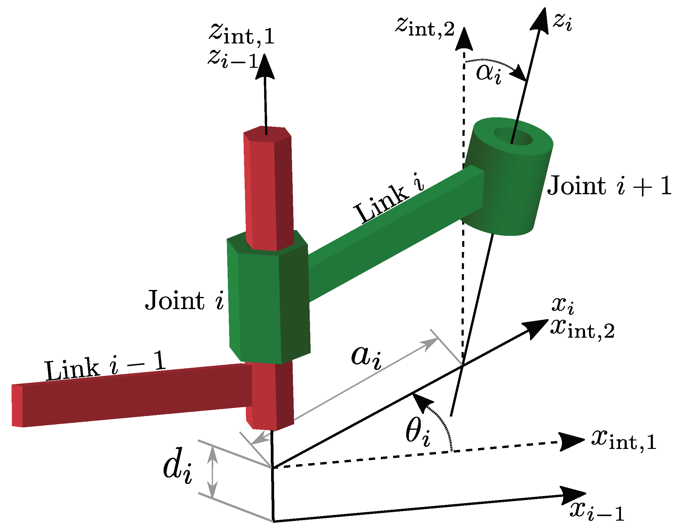
The Denavit-Hartenberg parameters, commonly referred to as DH parameters, are four geometric quantities that allow identifying the relative pose of a joint with respect to another in a systematic manner. We will denote a set of DH parameters as $\{d_i,{\theta }_i,a_i,{\alpha }_i\}$ for joint i. The parameters $d_i$ and ${\theta }_i$ are commonly referred to as joint parameters, while $a_i$ and ${\alpha }_i$ are known as the link parameters. A complete description of the DH parameters for R and P joint types, and several examples of their use are provided in [24]. In [24] a thorough description of the orientation of the frames is also provided, to which the reader is referred. In [25], Gan et al. have used dual quaternions in combination with the DH parameter convention to capture the pose transformation between joints. For completeness, we provide these equations herein, making use of Figure 2.

In words, the transformation from the reference frame assigned to the proximal joint (i.e., closer to the base of the robot) of a given link i, to the reference frame assigned to its distal joint (i.e., closer to the end effector), is described in terms of the DH parameters as:

• From the origin $O_{i-1}$, displace along the $Z_{i-1}$ (joint) axis by an amount $d_i$. Define this intermediate frame as $\{\mathrm{int},1\}$.
• Rotate about the $Z_{i-1}$ axis by ${\theta }_i$ until axis $X_{i-1}$ is superimposed to $X_i$
• Translate along $X_i$ by a distance of $a_i$. Define this intermediate frame as $\{\mathrm{int},2\}$.
• Rotate about the $X_i$ axis by ${\alpha }_i$

Mathematically, we can write this as the composition of four elementary dual quaternion operations, and summarize it further into two composite dual quaternions as

$$\begin{array}{}\mathrm{(44)}& \hfill {\mathit{q}}_{\mathrm{i}/\mathrm{i}-1}& =(\mathtt{1}+ϵr_{\mathrm{int},1/\mathrm{i}-1}^{\mathrm{int},1})(q_{\mathrm{int},2/\mathrm{int},1}+ϵ\mathtt{0})(\mathtt{1}+ϵr_{\mathrm{int},2/\mathrm{int},1}^{\mathrm{int},2})(q_{\mathrm{i}/\mathrm{int},2}+ϵ\mathtt{0})\hfill \mathrm{(45)}& & =(q_{\mathrm{int},2/\mathrm{int},1}+ϵr_{\mathrm{int},1/\mathrm{i}-1}^{\mathrm{int},1}{q}_{\mathrm{int},2/\mathrm{int},1})(q_{\mathrm{i}/\mathrm{int},2}+ϵr_{\mathrm{int},2/\mathrm{int},1}^{\mathrm{int},2}{q}_{\mathrm{i}/\mathrm{int},2})\hfill \end{array}$$

where

$$\begin{array}{cc}\hfill r_{\mathrm{int},1/\mathrm{i}-1}^{\mathrm{int},1}& =\left(0,{[0,0,d_i]}^{\mathrm{T}}\right)\hfill \end{array}$$

(46)

$$\begin{array}{cc}\hfill q_{\mathrm{int},2/\mathrm{int},1}& =\left(\cos {\theta }_i/2,{[0,0,sin{\theta }_i/2]}^{\mathrm{T}}\right)\hfill \end{array}$$

(47)

$$\begin{array}{cc}\hfill r_{\mathrm{int},2/\mathrm{int},1}^{\mathrm{int},2}& =\left(0,{[a_i,0,0]}^{\mathrm{T}}\right)\hfill \end{array}$$

(48)

$$\begin{array}{cc}\hfill q_{\mathrm{i}/\mathrm{int},2}& =\left(\cos {\alpha }_i/2,{[\sin {\alpha }_i/2,0,0]}^{\mathrm{T}}\right)\hfill \end{array}$$

(49)

Notice that while this is compact and readable up to multiplication of the dual quaternions, the same cannot be said about the end result compared to its homogeneous transformation matrix (HTM) counterpart. In fact, if we express ${\mathit{q}}_{\mathrm{i}/\mathrm{i}-1}$ component-wise, and cast it as a vector in ${\mathbb{R}}^8$ which is the typical representation of dual quaternions for numerical purposes, and compute the equivalent HTM, we get the following:

$$\begin{array}{c}\hfill {\mathit{q}}_{\mathrm{i}/\mathrm{i}-1}=\left[\begin{array}{c}cos(\alpha /2)cos(\theta /2)\\ sin(\alpha /2)cos(\theta /2)\\ sin(\alpha /2)sin(\theta /2)\\ cos(\alpha /2)sin(\theta /2)\\ -\frac{1}{2}{a}_{i}sin({\alpha }_i/2)cos({\theta }_i/2)-\frac{1}{2}{d}_{i}cos({\alpha }_i/2)sin({\theta }_i/2)\\ \frac{1}{2}{a}_{i}cos({\alpha }_i/2)cos({\theta }_i/2)-\frac{1}{2}{d}_{i}sin({\alpha }_i/2)sin({\theta }_i/2)\\ \frac{1}{2}{a}_{i}cos({\alpha }_i/2)sin({\theta }_i/2)+\frac{1}{2}{d}_{i}sin({\alpha }_i/2)cos({\theta }_i/2)\\ \frac{1}{2}{d}_{i}cos({\alpha }_i/2)cos({\theta }_i/2)-\frac{1}{2}{a}_{i}sin({\alpha }_i/2)sin({\theta }_i/2)\end{array}\right]\end{array}$$

(50)

$$T_{\mathrm{i}/\mathrm{i}-1}=\left[\begin{array}{cccc}\hfill cos{\theta }_i& sin{\theta }_i& 0\hfill & -a_i\\ \hfill -cos{\alpha }_{i}sin{\theta }_i& cos{\alpha }_{i}cos{\theta }_i& sin{\alpha }_i\hfill & -d_{i}sin{\alpha }_i\\ \hfill sin{\alpha }_{i}sin{\theta }_i& -sin{\alpha }_{i}cos{\theta }_i& cos{\alpha }_i\hfill & -d_{i}cos{\alpha }_i\\ \hfill 0& 0& 0\hfill & 1\end{array}\right].$$

(51)

While the HTM is more readable and faster to code, it uses 16 doubles and a multi-dimensional array to store the information and operate in the underlying algebra.

Remark 4.

Since the transformations associated to ${\theta }_i$ and $d_i$ are about $z_{i-1}$ and the operations associated to ${\alpha }_i$ and $a_i$ happen about $x_i$, both stages of the DH transformation can be interpreted in the context of screw theory. Hence, the operation described by Equation (44) can be equivalently expressed as the composition of exponential operations given by

$$q_{\mathrm{i}/\mathrm{i}-1}=exp(\frac{1}{2}{\mathit{\theta }}_1{\mathit{s}}_1)exp(\frac{1}{2}{\mathit{\theta }}_2{\mathit{s}}_2),$$

(52)

where ${\mathit{\theta }}_1={\theta }_i+ϵd_i$ and ${\mathit{s}}_1=(0,{[0,0,1]}^{\mathrm{T}})+ϵ\mathtt{0}$ and ${\mathit{\theta }}_2={\alpha }_i+ϵa_i$ and ${\mathit{s}}_2=(0,{[1,0,0]}^{\mathrm{T}})+ϵ\mathtt{0}$.

4. Manipulator Kinematics Using Dual Quaternions

In this section we provide examples to demonstrate how one can develop the kinematic equations for different types of serial manipulators using dual quaternions.

4.1. Example: Forward Kinematics with an Inertially Fixed Base

The serial RR configuration in Figure 3 will be used as an example of how to use dual quaternions for forward kinematics. Notice that the pose of the end effector with respect to the inertial frame is given by

$${\mathit{q}}_{\mathrm{e}/\mathrm{I}}={\mathit{q}}_{1/\mathrm{I}}{\mathit{q}}_{2/1}{\mathit{q}}_{\mathrm{e}/2}.$$

(53)

For the sake of exposition, these are given by

$$\begin{array}{cc}\hfill {\mathit{q}}_{1/\mathrm{I}}& =(\mathtt{1}+ϵ\frac{1}{2}{r}_{1/\mathrm{I}}^{\mathrm{I}})(q_{1/\mathrm{I}}+ϵ\mathtt{0}),\hfill \end{array}$$

(54)

$$\begin{array}{cc}\hfill {\mathit{q}}_{2/1}& =(\mathtt{1}+ϵ\frac{1}{2}{r}_{2/1}^1)(q_{2/1}+ϵ\mathtt{0}),\hfill \end{array}$$

(55)

$$\begin{array}{cc}\hfill {\mathit{q}}_{\mathrm{e}/2}& =(\mathtt{1}+ϵ\frac{1}{2}{r}_{\mathrm{e}/2}^2)(q_{\mathrm{e}/2}+ϵ\mathtt{0}),\hfill \end{array}$$

(56)

where the translation-first approach has been used. Each of these quantities can be easily determined from the geometry of the problem. The position quaternions are given by $r_{\mathrm{X}/\mathrm{Y}}^{\mathrm{Y}}=(0,{\overline{r}}_{\mathrm{X}/\mathrm{Y}}^{\mathrm{Y}})$, and

$$\begin{array}{c}\hfill {\overline{r}}_{1/\mathrm{I}}^{\mathrm{I}}={[0,0,0]}^{\mathrm{T}},\end{array}$$

(57)

$$\begin{array}{c}\hfill {\overline{r}}_{2/1}^1={[l_1,0,0]}^{\mathrm{T}},\end{array}$$

(58)

$$\begin{array}{c}\hfill {\overline{r}}_{\mathrm{e}/2}^2={[l_2,0,0]}^{\mathrm{T}},\end{array}$$

(59)

while the quaternions are given by

$$\begin{array}{cc}\hfill q_{1/\mathrm{I}}& =\left(\cos {\alpha }_1/2,{[0,0,sin{\alpha }_1/2]}^{\mathrm{T}}\right),\hfill \end{array}$$

(60)

$$\begin{array}{cc}\hfill q_{1/\mathrm{I}}& =\left(\cos {\alpha }_2/2,{[0,0,sin{\alpha }_2/2]}^{\mathrm{T}}\right),\hfill \end{array}$$

(61)

$$\begin{array}{cc}\hfill q_{\mathrm{e}/2}& =\mathtt{1}.\hfill \end{array}$$

(62)

The time derivative of the dual quaternion yields information about the angular and linear velocity of the end-effector. In particular, we have that for a dual quaternion:

$$\begin{array}{c}\hfill {\dot{\mathit{q}}}_{\mathrm{X}/\mathrm{Y}}=\frac{1}{2}{\mathit{q}}_{\mathrm{X}/\mathrm{Y}}{\mathit{\omega }}_{\mathrm{X}/\mathrm{Y}}^{\mathrm{X}}=\frac{1}{2}{\mathit{\omega }}_{\mathrm{X}/\mathrm{Y}}^{\mathrm{Y}}{\mathit{q}}_{\mathrm{X}/\mathrm{Y}},\end{array}$$

(63)

where the first equality in Equation (63) is associated with a body-frame time derivative, and the second equality in Equation (63) is associated with a spatial-frame time derivative.

With these definitions in mind, we compute the time-rate of change of the pose of the end-effector as

$$\begin{array}{}\mathrm{(64)}& \hfill {\dot{\mathit{q}}}_{\mathrm{e}/\mathrm{I}}& ={\dot{\mathit{q}}}_{1/\mathrm{I}}{\mathit{q}}_{2/1}{\mathit{q}}_{\mathrm{e}/2}+{\mathit{q}}_{1/\mathrm{I}}{\dot{\mathit{q}}}_{2/1}{\mathit{q}}_{\mathrm{e}/2}+{\mathit{q}}_{1/\mathrm{I}}{\mathit{q}}_{2/1}{\dot{\mathit{q}}}_{\mathrm{e}/2}\hfill \mathrm{(65)}& & =\frac{1}{2}{\mathit{q}}_{1/\mathrm{I}}{\mathit{\omega }}_{1/\mathrm{I}}^1{\mathit{q}}_{2/1}{\mathit{q}}_{\mathrm{e}/2}+{\mathit{q}}_{1/\mathrm{I}}\frac{1}{2}{\mathit{q}}_{2/1}{\mathit{\omega }}_{2/1}^2{\mathit{q}}_{\mathrm{e}/2}+{\mathit{q}}_{1/\mathrm{I}}{\mathit{q}}_{2/1}\frac{1}{2}{\mathit{q}}_{\mathrm{e}/2}{\mathit{\omega }}_{\mathrm{e}/2}^{\mathrm{e}}.\hfill \end{array}$$

Then, using Equation (63), we get that the dual velocity of the end effector with respect to the inertial frame is given by

$$\begin{array}{}& \hfill {\mathit{\omega }}_{\mathrm{e}/\mathrm{I}}^{\mathrm{e}}& =2{\mathit{q}}_{\mathrm{e}/\mathrm{I}}^{*}{\dot{\mathit{q}}}_{\mathrm{e}/\mathrm{I}}\hfill & & ={\mathit{q}}_{\mathrm{e}/\mathrm{I}}^{*}{\mathit{q}}_{1/\mathrm{I}}{\mathit{\omega }}_{1/\mathrm{I}}^1{\mathit{q}}_{2/1}{\mathit{q}}_{\mathrm{e}/2}+{\mathit{q}}_{\mathrm{e}/\mathrm{I}}^{*}{\mathit{q}}_{1/\mathrm{I}}{\mathit{q}}_{2/1}{\mathit{\omega }}_{2/1}^2{\mathit{q}}_{\mathrm{e}/2}+{\mathit{q}}_{\mathrm{e}/\mathrm{I}}^{*}{\mathit{q}}_{1/\mathrm{I}}{\mathit{q}}_{2/1}{\mathit{q}}_{\mathrm{e}/2}\stackrel{=\mathbf{0}}{\overbrace{{\mathit{\omega }}_{\mathrm{e}/2}^{\mathrm{e}}}}\hfill & & ={\mathit{q}}_{\mathrm{e}/2}^{*}{\mathit{q}}_{2/1}^{*}{\mathit{q}}_{1/\mathrm{I}}^{*}{\mathit{q}}_{1/\mathrm{I}}{\mathit{\omega }}_{1/\mathrm{I}}^1{\mathit{q}}_{2/1}{\mathit{q}}_{\mathrm{e}/2}+{\mathit{q}}_{\mathrm{e}/2}^{*}{\mathit{q}}_{2/1}^{*}{\mathit{q}}_{1/\mathrm{I}}^{*}{\mathit{q}}_{1/\mathrm{I}}{\mathit{q}}_{2/1}{\mathit{\omega }}_{2/1}^2{\mathit{q}}_{\mathrm{e}/2}\hfill & & ={\mathit{q}}_{\mathrm{e}/2}^{*}{\mathit{q}}_{2/1}^{*}{\mathit{\omega }}_{1/\mathrm{I}}^1{\mathit{q}}_{2/1}{\mathit{q}}_{\mathrm{e}/2}+{\mathit{q}}_{\mathrm{e}/2}^{*}{\mathit{\omega }}_{2/1}^2{\mathit{q}}_{\mathrm{e}/2}\hfill & & ={\mathrm{Ad}}_{{\mathit{q}}_{\mathrm{e}/2}^{*}{\mathit{q}}_{2/1}^{*}}{\mathit{\omega }}_{1/\mathrm{I}}^1+{\mathrm{Ad}}_{{\mathrm{q}}_{\mathrm{e}/2}^{*}}{\mathit{\omega }}_{2/1}^2\hfill & & ={\mathrm{Ad}}_{{({\mathit{q}}_{2/1}{\mathit{q}}_{\mathrm{e}/2})}^{*}}{\mathit{\omega }}_{1/\mathrm{I}}^1+{\mathrm{Ad}}_{{({\mathrm{q}}_{\mathrm{e}/2})}^{*}}{\mathit{\omega }}_{2/1}^2\hfill \mathrm{(66)}& & =\left[{\mathrm{Ad}}_{{({\mathit{q}}_{2/1}{\mathit{q}}_{\mathrm{e}/2})}^{*}}{\mathit{\xi }}_{1/\mathrm{I}}^1,{\mathrm{Ad}}_{{({\mathrm{q}}_{\mathrm{e}/2})}^{*}}{\mathit{\xi }}_{2/1}^2\right]\dot{\overline{\alpha }}\hfill \mathrm{(67)}& & =J^{\mathrm{B}}(\mathit{q},\mathit{\xi })\dot{\overline{\alpha }},\hfill \end{array}$$

where $J^{\mathrm{B}}(\mathit{q},\mathit{\xi })$ is the Jacobian expressed in the body frame and

$$\overline{\alpha }=\left[\begin{array}{c}{\alpha }_1\\ {\alpha }_2\end{array}\right]\mathrm{and}\dot{\overline{\alpha }}=\left[\begin{array}{c}{\dot{\alpha }}_1\\ {\dot{\alpha }}_2\end{array}\right].$$

(68)

The elements ${\mathit{\xi }}_i$ are the dual quaternion screws for each of the joints. In general, the screws for revolute and prismatic joints are listed in

Table 4. Screw (${\mathit{\xi }}_i$) for revolute and prismatic joints.

	Revolute Joint	Prismatic Joint
X-axis	$(0,{[1,0,0]}^{\mathrm{T}})+ϵ\mathtt{0}$	$\mathtt{0}+ϵ(0,{[1,0,0]}^{\mathrm{T}})$
Y-axis	$(0,{[0,1,0]}^{\mathrm{T}})+ϵ\mathtt{0}$	$\mathtt{0}+ϵ(0,{[0,1,0]}^{\mathrm{T}})$
Z-axis	$(0,{[0,0,1]}^{\mathrm{T}})+ϵ\mathtt{0}$	$\mathtt{0}+ϵ(0,{[0,0,1]}^{\mathrm{T}})$

for each of the three axes, and these are independent of the current robot configuration.

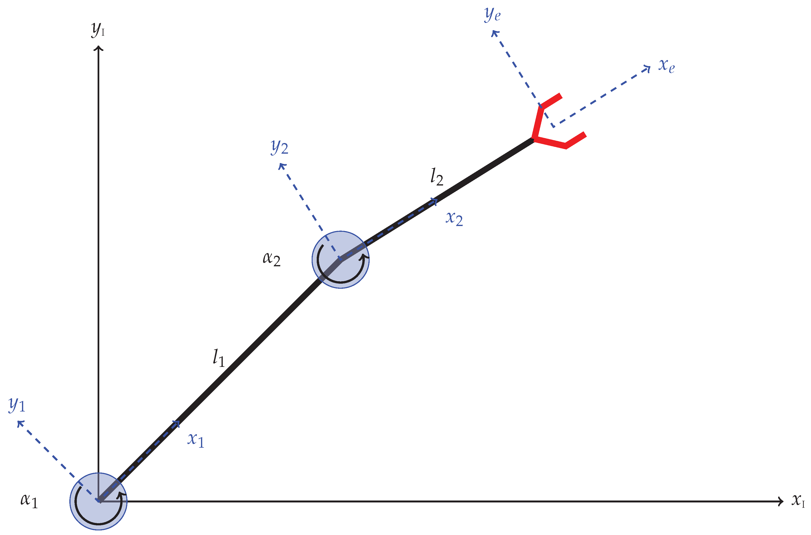
4.2. Example: Forward Kinematics of a Floating Double Pendulum with End-Effector

Given the floating double pendulum shown in Figure 4, we want to model its kinematics. The difference with respect to the one shown in Figure 3 is that the first revolute joint is free to translate in 2D space.

The kinematic equations of motion can thus be derived as follows using a geometric description of the forward kinematics

$${\mathit{q}}_{\mathrm{e}/\mathrm{I}}={\mathit{q}}_{1/\mathrm{I}}{\mathit{q}}_{2/1}{\mathit{q}}_{\mathrm{e}/2},$$

(69)

where ${\mathit{q}}_{1/\mathrm{I}}$, ${\mathit{q}}_{2/1}$, ${\mathit{q}}_{\mathrm{e}/2}$ are given by Equations (54)–(56). However, ${\overline{r}}_{1/\mathrm{I}}^{\mathrm{I}}={[u,v,0]}^{\mathrm{T}}$ determines the translation of the first revolute joint in 2D. It is clear that

$$\frac{\mathrm{d}}{\mathrm{d}t}{\overline{r}}_{1/\mathrm{I}}^{\mathrm{I}}={\dot{\overline{r}}}_{1/\mathrm{I}}^{\mathrm{I}}={\overline{v}}_{1/\mathrm{I}}^{\mathrm{I}}={[\dot{u},\dot{v},0]}^{\mathrm{T}}$$

(70)

In this case, the time evolution of ${\mathit{q}}_{1/\mathrm{I}}$ is given by

$${\dot{\mathit{q}}}_{1/\mathrm{I}}=\frac{1}{2}{\mathit{\omega }}_{1/\mathrm{I}}^{\mathrm{I}}{\mathit{q}}_{1/\mathrm{I}}$$

(71)

as before, but we redefine the dual velocity as dictated by the definition in Equation (14) as

$${\mathit{\omega }}_{1/\mathrm{I}}^{\mathrm{I}}={\omega }_{1/\mathrm{I}}^{\mathrm{I}}+ϵ(v_{1/\mathrm{I}}^{\mathrm{I}}-{\omega }_{1/\mathrm{I}}^{\mathrm{I}}\times r_{1/\mathrm{I}}^{\mathrm{I}}).$$

(72)

The relationship derived earlier

$$\begin{array}{cc}\hfill {\mathit{\omega }}_{\mathrm{e}/\mathrm{I}}^{\mathrm{e}}& ={\mathrm{Ad}}_{{\mathit{q}}_{\mathrm{e}/2}^{*}{\mathit{q}}_{2/1}^{*}}{\mathit{\omega }}_{1/\mathrm{I}}^1+{\mathrm{Ad}}_{{\mathrm{q}}_{\mathrm{e}/2}^{*}}{\omega }_{2/1}^2\hfill \end{array}$$

still holds. However, ${\mathit{\omega }}_{1/\mathrm{I}}^1$ must be computed from our knowledge of ${\mathit{\omega }}_{1/\mathrm{I}}^{\mathrm{I}}$. While in quaternion and vector notation this might be troublesome, the expression using dual quaternions is simple and given by

$${\mathit{\omega }}_{1/\mathrm{I}}^1={\mathit{q}}_{1/\mathrm{I}}^{*}{\mathit{\omega }}_{1/\mathrm{I}}^{\mathrm{I}}{\mathit{q}}_{1/\mathrm{I}}={\mathrm{Ad}}_{{\mathit{q}}_{1/\mathrm{I}}^{*}}{\mathit{\omega }}_{1/\mathrm{I}}^{\mathrm{I}}.$$

(73)

4.3. Manipulator on an Orbiting Spacecraft

For the general case, the robot base can move with six degrees of freedom, reinforcing the need for a convenient pose representation tool such as dual quaternions. Following an approach analogous to that proposed by Adorno in [26], in this section we will provide explicit expressions for the Jacobian matrix for different types of joints.

The kinematics of the robotic base, attached to frame $\mathrm{B}$, would still be governed by the equation

$${\dot{\mathit{q}}}_{\mathrm{B}/\mathrm{I}}=\frac{1}{2}{\mathit{q}}_{\mathrm{B}/\mathrm{I}}{\mathit{\omega }}_{\mathrm{B}/\mathrm{I}}^{\mathrm{B}},$$

(74)

while the kinematics of the joints depend on the type of joint. The dual velocities for the joints depend on frame positioning and on the selection of the generalized coordinates. In

Table 5. Generalized coordinates and dual velocities for different joint types.

Joint Type	Generalized Coordinate Parametrization, ${\overline{\mathit{\alpha }}}_{\mathit{i}}$	Dual Velocity, ${\mathit{\omega }}_{\mathbf{i}/\mathbf{i}-1}^{\mathbf{i}}$
Revolute	${\theta }_{\mathrm{i}/\mathrm{i}-1}\in {\mathbb{R}}^1$	$(0,{[0,0,{\dot{\theta }}_{\mathrm{i}/\mathrm{i}-1}]}^{\mathrm{T}})+ϵ\mathtt{0}$
Prismatic	$z_{\mathrm{i}/\mathrm{i}-1}\in {\mathbb{R}}^1$	$\mathtt{0}+ϵ(0,{[0,0,{\dot{z}}_{\mathrm{i}/\mathrm{i}-1}]}^{\mathrm{T}})$
Spherical	${[{\varphi }_{\mathrm{i}/\mathrm{i}-1},{\theta }_{\mathrm{i}/\mathrm{i}-1},{\psi }_{\mathrm{i}/\mathrm{i}-1}]}^{\mathrm{T}}\in {\mathbb{R}}^3$	$(0,M({\varphi }_{\mathrm{i}/\mathrm{i}-1},{\theta }_{\mathrm{i}/\mathrm{i}-1},{\psi }_{\mathrm{i}/\mathrm{i}-1}){[{\dot{\varphi }}_{\mathrm{i}/\mathrm{i}-1},{\dot{\theta }}_{\mathrm{i}/\mathrm{i}-1},{\dot{\psi }}_{\mathrm{i}/\mathrm{i}-1}]}^{\mathrm{T}})+ϵ\mathtt{0}$
Cylindrical	${[{\theta }_{\mathrm{i}/\mathrm{i}-1},z_{\mathrm{i}/\mathrm{i}-1}]}^{\mathrm{T}}\in {\mathbb{R}}^2$	$(0,{[0,0,{\dot{\theta }}_{\mathrm{i}/\mathrm{i}-1}]}^{\mathrm{T}})+ϵ(0,{[0,0,{\dot{z}}_{\mathrm{i}/\mathrm{i}-1}]}^{\mathrm{T}})$
Cartesian	${[x_{\mathrm{i}/\mathrm{i}-1},y_{\mathrm{i}/\mathrm{i}-1},z_{\mathrm{i}/\mathrm{i}-1}]}^{\mathrm{T}}\in {\mathbb{R}}^3$	$\mathtt{0}+ϵ(0,{[{\dot{x}}_{\mathrm{i}/\mathrm{i}-1},{\dot{y}}_{\mathrm{i}/\mathrm{i}-1},{\dot{z}}_{\mathrm{i}/\mathrm{i}-1}]}^{\mathrm{T}})$

, we provide example generalized coordinates and their corresponding dual velocities. Simple numerical derivatives can yield the dual acceleration of the joint. It is worth emphasizing that for a $3-2-1/\psi -\theta -\varphi$ rotation, the matrix $M({\varphi }_{\mathrm{i}/\mathrm{i}-1},{\theta }_{\mathrm{i}/\mathrm{i}-1},{\psi }_{\mathrm{i}/\mathrm{i}-1})$ will correspond to

$$M({\varphi }_{\mathrm{i}/\mathrm{i}-1},{\theta }_{\mathrm{i}/\mathrm{i}-1},{\psi }_{\mathrm{i}/\mathrm{i}-1})=\left[\begin{array}{ccc}1& 0& -sin\left({\theta }_{\mathrm{i}/\mathrm{i}-1}\right)\\ 0& cos\left({\varphi }_{\mathrm{i}/\mathrm{i}-1}\right)& cos\left({\theta }_{\mathrm{i}/\mathrm{i}-1}\right)sin\left({\varphi }_{\mathrm{i}/\mathrm{i}-1}\right)\\ 0& -sin\left({\varphi }_{\mathrm{i}/\mathrm{i}-1}\right)& cos\left({\theta }_{\mathrm{i}/\mathrm{i}-1}\right)cos\left({\varphi }_{\mathrm{i}/\mathrm{i}-1}\right)\end{array}\right].$$

(75)

In general, we can identify the pose of a satellite-mounted end-effector by

$${\mathit{q}}_{\mathrm{e}/\mathrm{I}}={\mathit{q}}_{\mathrm{B}/\mathrm{I}}{\mathit{q}}_{\mathrm{O}/\mathrm{B}}{\mathit{q}}_{0/\mathrm{O}}\left(\prod _{\mathrm{i}=1}^{n-1}{q}_{\mathrm{i}/\mathrm{i}-1}\right){\mathit{q}}_{\mathrm{e}/\mathrm{n}-1},$$

(76)

where ${\mathit{q}}_{\mathrm{O}/\mathrm{B}}$ represents the pose transformation from the body frame of the satellite, $\mathrm{B}$, to the frame at the base of the satellite manipulator, denoted by O; frame $\mathrm{i}$ represents the joint frame attached to the $\mathrm{i}$-th link, one of the $\mathrm{n}$ bodies composing the manipulator, at the location of the proximal joint; and $\mathrm{e}$ is the end-effector frame that is rigidly attached to the last link of the serial manipulator, $\mathrm{n}-1$. For clarity, an example of the product operator ∏ used on dual quaternions is given by

$$\prod _{i=1}^2{\mathit{q}}_{\mathrm{i}/\mathrm{i}-1}={\mathit{q}}_{1/0}{\mathit{q}}_{2/1}.$$

(77)

Additionally, using the definition of frames described above, the first link of the manipulator is link 0 and its connecting joint to the satellite base is frame 0.

Then, since ${\mathit{q}}_{\mathrm{O}/\mathrm{B}}$ and ${\mathit{q}}_{\mathrm{e}/\mathrm{n}-1}$ are constant, the kinematics can be derived following the procedure of previous sections as

$$\begin{array}{cc}\hfill {\dot{\mathit{q}}}_{\mathrm{e}/\mathrm{I}}& ={\dot{\mathit{q}}}_{\mathrm{B}/\mathrm{I}}{\mathit{q}}_{\mathrm{O}/\mathrm{B}}{\mathit{q}}_{0/\mathrm{O}}\left(\prod _{\mathrm{i}=1}^{\mathrm{n}-1}{\mathit{q}}_{\mathrm{i}/\mathrm{i}-1}\right){\mathit{q}}_{\mathrm{e}/\mathrm{n}-1}+{\mathit{q}}_{\mathrm{B}/\mathrm{I}}{\mathit{q}}_{\mathrm{O}/\mathrm{B}}{\dot{\mathit{q}}}_{0/\mathrm{O}}\left(\prod _{\mathrm{i}=1}^{\mathrm{n}-1}{\mathit{q}}_{\mathrm{i}/\mathrm{i}-1}\right){\mathit{q}}_{\mathrm{e}/\mathrm{n}-1}\hfill \\ & +{\mathit{q}}_{\mathrm{B}/\mathrm{I}}{\mathit{q}}_{\mathrm{O}/\mathrm{B}}{\mathit{q}}_{0/\mathrm{O}}\sum _{\mathrm{k}=1}^{\mathrm{n}-1}\left({\mathit{q}}_{\mathrm{k}-1/0}{\dot{\mathit{q}}}_{\mathrm{k}/\mathrm{k}-1}{\mathit{q}}_{\mathrm{n}-1/\mathrm{k}}\right){\mathit{q}}_{\mathrm{e}/\mathrm{n}-1}\hfill \\ & =\frac{1}{2}{\mathit{q}}_{\mathrm{B}/\mathrm{I}}{\mathit{\omega }}_{\mathrm{B}/\mathrm{I}}^{\mathrm{B}}{\mathit{q}}_{\mathrm{O}/\mathrm{B}}{\mathit{q}}_{0/\mathrm{O}}\left(\prod _{\mathrm{i}=1}^{\mathrm{n}-1}{\mathit{q}}_{\mathrm{i}/\mathrm{i}-1}\right){\mathit{q}}_{\mathrm{e}/\mathrm{n}-1}+{\mathit{q}}_{\mathrm{B}/\mathrm{I}}{\mathit{q}}_{\mathrm{O}/\mathrm{B}}\frac{1}{2}{\mathit{q}}_{0/\mathrm{O}}{\mathit{\omega }}_{0/\mathrm{O}}^0\left(\prod _{\mathrm{i}=1}^{\mathrm{n}-1}{\mathit{q}}_{\mathrm{i}/\mathrm{i}-1}\right){\mathit{q}}_{\mathrm{e}/\mathrm{n}-1}\hfill \\ & +{\mathit{q}}_{\mathrm{B}/\mathrm{I}}{\mathit{q}}_{\mathrm{O}/\mathrm{B}}{\mathit{q}}_{0/\mathrm{O}}\sum _{\mathrm{k}=1}^{\mathrm{n}-1}\left({\mathit{q}}_{\mathrm{k}-1/0}\frac{1}{2}{\mathit{q}}_{\mathrm{k}/\mathrm{k}-1}{\mathit{\omega }}_{\mathrm{k}/\mathrm{k}-1}^{\mathrm{k}}{\mathit{q}}_{\mathrm{n}-1/\mathrm{k}}\right){\mathit{q}}_{\mathrm{e}/\mathrm{n}-1}.\hfill \end{array}$$

(78)

Multiplying by $2{\mathit{q}}_{\mathrm{e}/\mathrm{I}}^{*}$ on the left, we get

$$\begin{array}{cc}\hfill {\mathit{\omega }}_{\mathrm{e}/\mathrm{I}}^{\mathrm{e}}& ={\mathit{q}}_{\mathrm{e}/\mathrm{I}}^{*}{\mathit{q}}_{\mathrm{B}/\mathrm{I}}{\mathit{\omega }}_{\mathrm{B}/\mathrm{I}}^{\mathrm{B}}{\mathit{q}}_{\mathrm{O}/\mathrm{B}}{\mathit{q}}_{0/\mathrm{O}}\left(\prod _{\mathrm{i}=1}^{\mathrm{n}-1}{\mathit{q}}_{\mathrm{i}/\mathrm{i}-1}\right){\mathit{q}}_{\mathrm{e}/\mathrm{n}-1}+{\mathit{q}}_{\mathrm{e}/\mathrm{I}}^{*}{\mathit{q}}_{\mathrm{B}/\mathrm{I}}{\mathit{q}}_{\mathrm{O}/\mathrm{B}}{\mathit{q}}_{0/\mathrm{O}}{\mathit{\omega }}_{0/\mathrm{O}}^0\left(\prod _{\mathrm{i}=1}^{\mathrm{n}-1}{\mathit{q}}_{\mathrm{i}/\mathrm{i}-1}\right){\mathit{q}}_{\mathrm{e}/\mathrm{n}-1}\hfill \\ & +{\mathit{q}}_{\mathrm{e}/\mathrm{I}}^{*}{\mathit{q}}_{\mathrm{B}/\mathrm{I}}{\mathit{q}}_{\mathrm{O}/\mathrm{B}}{\mathit{q}}_{0/\mathrm{O}}\sum _{\mathrm{k}=1}^{\mathrm{n}-1}\left({\mathit{q}}_{\mathrm{k}-1/0}{\mathit{q}}_{\mathrm{k}/\mathrm{k}-1}{\mathit{\omega }}_{\mathrm{k}/\mathrm{k}-1}^{\mathrm{k}}{\mathit{q}}_{\mathrm{n}-1/\mathrm{k}}\right){\mathit{q}}_{\mathrm{e}/\mathrm{n}-1},\hfill \end{array}$$

(79)

and carrying out the dual quaternion multiplications to simplify the expression yields

$$\begin{array}{c}\hfill {\mathit{\omega }}_{\mathrm{e}/\mathrm{I}}^{\mathrm{e}}={\mathit{q}}_{\mathrm{e}/\mathrm{B}}^{*}{\mathit{\omega }}_{\mathrm{B}/\mathrm{I}}^{\mathrm{B}}{\mathit{q}}_{\mathrm{e}/\mathrm{B}}+{\mathit{q}}_{\mathrm{e}/0}^{*}{\mathit{\omega }}_{0/\mathrm{O}}^0{\mathit{q}}_{\mathrm{e}/0}+\sum _{\mathrm{k}=1}^{\mathrm{n}-1}{\mathit{q}}_{\mathrm{e}/\mathrm{k}}^{*}{\mathit{\omega }}_{\mathrm{k}/\mathrm{k}-1}^{\mathrm{k}}{\mathit{q}}_{\mathrm{e}/\mathrm{k}}.\end{array}$$

(80)

In this form, it is straightforward to identify that in Equation (80), the first term yields the motion of the end-effector due to the motion of the base. The second and third terms provide the effect of the motion of the end-effector due to joint motion. We can now manipulate Equation (80) towards a more familiar structure

$$\begin{array}{cc}\hfill {\mathit{\omega }}_{\mathrm{e}/\mathrm{I}}^{\mathrm{e}}& =⟦\phantom{{\mathit{q}}_{\mathrm{e}/\mathrm{B}}^{*}}{\mathit{q}}_{\mathrm{e}/\mathrm{B}}^{*}{\phantom{{\mathit{q}}_{\mathrm{e}/\mathrm{B}}^{*}}⟧}_{\mathrm{L}}⟦\phantom{{\mathit{q}}_{\mathrm{e}/\mathrm{B}}}{\mathit{q}}_{\mathrm{e}/\mathrm{B}}{\phantom{{\mathit{q}}_{\mathrm{e}/\mathrm{B}}}⟧}_{\mathrm{R}}\star {\mathit{\omega }}_{\mathrm{B}/\mathrm{I}}^{\mathrm{B}}+⟦\phantom{{\mathit{q}}_{\mathrm{e}/0}^{*}}{\mathit{q}}_{\mathrm{e}/0}^{*}{\phantom{{\mathit{q}}_{\mathrm{e}/0}^{*}}⟧}_{\mathrm{L}}⟦\phantom{{\mathit{q}}_{\mathrm{e}/0}}{\mathit{q}}_{\mathrm{e}/0}{\phantom{{\mathit{q}}_{\mathrm{e}/0}}⟧}_{\mathrm{R}}\star {\mathit{\omega }}_{0/\mathrm{O}}^0+\sum _{\mathrm{k}=1}^{\mathrm{n}-1}⟦\phantom{{\mathit{q}}_{\mathrm{e}/\mathrm{k}}^{*}}{\mathit{q}}_{\mathrm{e}/\mathrm{k}}^{*}{\phantom{{\mathit{q}}_{\mathrm{e}/\mathrm{k}}^{*}}⟧}_{\mathrm{L}}⟦\phantom{{\mathit{q}}_{\mathrm{e}/\mathrm{k}}}{\mathit{q}}_{\mathrm{e}/\mathrm{k}}{\phantom{{\mathit{q}}_{\mathrm{e}/\mathrm{k}}}⟧}_{\mathrm{R}}\star {\mathit{\omega }}_{\mathrm{k}/\mathrm{k}-1}^{\mathrm{k}}.\hfill \end{array}$$

(81)

Defining the vector of generalized coordinates as the vertical concatenation of the individual joint generalized coordinates, we can write

$$\begin{array}{cc}\hfill {\mathit{\omega }}_{\mathrm{e}/\mathrm{I}}^{\mathrm{e}}& =⟦\phantom{{\mathit{q}}_{\mathrm{e}/\mathrm{B}}^{*}}{\mathit{q}}_{\mathrm{e}/\mathrm{B}}^{*}{\phantom{{\mathit{q}}_{\mathrm{e}/\mathrm{B}}^{*}}⟧}_{\mathrm{L}}⟦\phantom{{\mathit{q}}_{\mathrm{e}/\mathrm{B}}}{\mathit{q}}_{\mathrm{e}/\mathrm{B}}{\phantom{{\mathit{q}}_{\mathrm{e}/\mathrm{B}}}⟧}_{\mathrm{R}}\star {\mathit{\omega }}_{\mathrm{B}/\mathrm{I}}^{\mathrm{B}}+⟦\phantom{{\mathit{q}}_{\mathrm{e}/0}^{*}}{\mathit{q}}_{\mathrm{e}/0}^{*}{\phantom{{\mathit{q}}_{\mathrm{e}/0}^{*}}⟧}_{\mathrm{L}}⟦\phantom{{\mathit{q}}_{\mathrm{e}/0}}{\mathit{q}}_{\mathrm{e}/0}{\phantom{{\mathit{q}}_{\mathrm{e}/0}}⟧}_{\mathrm{R}}{\zeta }_0{\dot{\overline{\alpha }}}_0+\sum _{\mathrm{k}=1}^{\mathrm{n}-1}⟦\phantom{{\mathit{q}}_{\mathrm{e}/\mathrm{k}}^{*}}{\mathit{q}}_{\mathrm{e}/\mathrm{k}}^{*}{\phantom{{\mathit{q}}_{\mathrm{e}/\mathrm{k}}^{*}}⟧}_{\mathrm{L}}⟦\phantom{{\mathit{q}}_{\mathrm{e}/\mathrm{k}}}{\mathit{q}}_{\mathrm{e}/\mathrm{k}}{\phantom{{\mathit{q}}_{\mathrm{e}/\mathrm{k}}}⟧}_{\mathrm{R}}{\zeta }_{\mathrm{k}}{\dot{\overline{\alpha }}}_{\mathrm{k}}\hfill \\ & =⟦\phantom{{\mathit{q}}_{\mathrm{e}/\mathrm{B}}^{*}}{\mathit{q}}_{\mathrm{e}/\mathrm{B}}^{*}{\phantom{{\mathit{q}}_{\mathrm{e}/\mathrm{B}}^{*}}⟧}_{\mathrm{L}}⟦\phantom{{\mathit{q}}_{\mathrm{e}/\mathrm{B}}}{\mathit{q}}_{\mathrm{e}/\mathrm{B}}{\phantom{{\mathit{q}}_{\mathrm{e}/\mathrm{B}}}⟧}_{\mathrm{R}}\star {\mathit{\omega }}_{\mathrm{B}/\mathrm{I}}^{\mathrm{B}}+J(\mathit{q},\zeta )\dot{\overline{\alpha }}.\hfill \end{array}$$

(82)

Here, we have defined the body-frame Jacobian associated to joint motion as

$$J(\mathit{q},\zeta )\triangleq \left[⟦\phantom{{\mathit{q}}_{\mathrm{e}/0}^{*}}{\mathit{q}}_{\mathrm{e}/0}^{*}{\phantom{{\mathit{q}}_{\mathrm{e}/0}^{*}}⟧}_{\mathrm{L}}⟦\phantom{{\mathit{q}}_{\mathrm{e}/0}}{\mathit{q}}_{\mathrm{e}/0}{\phantom{{\mathit{q}}_{\mathrm{e}/0}}⟧}_{\mathrm{R}}{\zeta }_0,\dots ,⟦\phantom{{\mathit{q}}_{\mathrm{e}/\mathrm{k}}^{*}}{\mathit{q}}_{\mathrm{e}/\mathrm{k}}^{*}{\phantom{{\mathit{q}}_{\mathrm{e}/\mathrm{k}}^{*}}⟧}_{\mathrm{L}}⟦\phantom{{\mathit{q}}_{\mathrm{e}/\mathrm{k}}}{\mathit{q}}_{\mathrm{e}/\mathrm{k}}{\phantom{{\mathit{q}}_{\mathrm{e}/\mathrm{k}}}⟧}_{\mathrm{R}}{\zeta }_{\mathrm{k}},\dots ,⟦\phantom{{\mathit{q}}_{\mathrm{e}/\mathrm{n}-1}^{*}}{\mathit{q}}_{\mathrm{e}/\mathrm{n}-1}^{*}{\phantom{{\mathit{q}}_{\mathrm{e}/\mathrm{n}-1}^{*}}⟧}_{\mathrm{L}}⟦\phantom{{\mathit{q}}_{\mathrm{e}/\mathrm{n}-1}}{\mathit{q}}_{\mathrm{e}/\mathrm{n}-1}{\phantom{{\mathit{q}}_{\mathrm{e}/\mathrm{n}-1}}⟧}_{\mathrm{R}}{\zeta }_{\mathrm{n}-1}\right].$$

(83)

The general term of the Jacobian mapping matrix, $⟦\phantom{{\mathit{q}}_{\mathrm{e}/\mathrm{k}}^{*}}{\mathit{q}}_{\mathrm{e}/\mathrm{k}}^{*}{\phantom{{\mathit{q}}_{\mathrm{e}/\mathrm{k}}^{*}}⟧}_{\mathrm{L}}⟦\phantom{{\mathit{q}}_{\mathrm{e}/\mathrm{k}}}{\mathit{q}}_{\mathrm{e}/\mathrm{k}}{\phantom{{\mathit{q}}_{\mathrm{e}/\mathrm{k}}}⟧}_{\mathrm{R}}{\zeta }_{\mathrm{k}}$, where ${\zeta }_{\mathrm{k}}$ is a screw matrix as defined in

Table 6. Screw matrix for different joint types.

Joint Type	Screw Matrix, ${\mathit{\zeta }}_{\mathbf{i}}=\mathit{\partial }{\mathit{\omega }}_{\mathbf{i}/\mathbf{i}-1}^{\mathit{i}}/\mathit{\partial }{\dot{\overline{\mathit{\alpha }}}}_{\mathit{i}}$
Revolute	${[0,0,0,1,0,0,0,0]}^{\mathrm{T}}$
Prismatic	${[0,0,0,0,0,0,0,1]}^{\mathrm{T}}$
Spherical	$\left[\begin{array}{c}{0}_{1\times 3}\\ M({\varphi }_{\mathrm{i}/\mathrm{i}-1},{\theta }_{\mathrm{i}/\mathrm{i}-1},{\psi }_{\mathrm{i}/\mathrm{i}-1})\\ 0_{4\times 4}\end{array}\right]$
Cylindrical	${\left[\begin{array}{c}0,0,0,1,0,0,0,0\\ 0,0,0,0,0,0,0,1\end{array}\right]}^{\mathrm{T}}$
Cartesian	$\left[\begin{array}{c}{0}_{5\times 3}\\ {\mathbb{I}}_3\end{array}\right]$

, is an improvement upon the more typical, adjoint-based methodology due to the ability of ${\zeta }_{\mathrm{k}}$ to capture more than one degree of freedom in each of its different columns. For the case in which the adjoint formula ${\mathrm{Ad}}_{{\mathit{q}}_{\mathrm{e}/\mathrm{k}}^{*}}{\mathit{\xi }}_{\mathrm{k}}$ is used, as in Equation (66), then ${\mathit{\xi }}_{\mathrm{k}}$ necessarily corresponds to one single generalized coordinate. In other words, the screws for the cylindrical, spherical and Cartesian joints would need to be separated into different columns, each of which has its adjoint operation applied independently.

For example, it would be easy to demonstrate that for a cylindrical $(d=2)$, spherical $(d=3)$ or Cartesian joints $(d=3)$,

$$\begin{array}{c}\hfill \frac{\partial {\mathit{\omega }}_{\mathrm{i}/\mathrm{i}-1}^{\mathrm{i}}}{\partial {\dot{\overline{\alpha }}}_{\mathrm{k}}}\equiv ⟦\phantom{{\mathit{q}}_{\mathrm{e}/\mathrm{k}}^{*}}{\mathit{q}}_{\mathrm{e}/\mathrm{k}}^{*}{\phantom{{\mathit{q}}_{\mathrm{e}/\mathrm{k}}^{*}}⟧}_{\mathrm{L}}⟦\phantom{{\mathit{q}}_{\mathrm{e}/\mathrm{k}}}{\mathit{q}}_{\mathrm{e}/\mathrm{k}}{\phantom{{\mathit{q}}_{\mathrm{e}/\mathrm{k}}}⟧}_{\mathrm{R}}{\zeta }_{\mathrm{k}}\in {\mathbb{R}}^{8\times d},\end{array}$$

(84)

but

$$\begin{array}{c}\hfill \frac{\partial {\mathit{\omega }}_{\mathrm{i}/\mathrm{i}-1}^{\mathrm{i}}}{\partial {\dot{\overline{\alpha }}}_{\mathrm{k}}}\ne {\mathrm{Ad}}_{{\mathit{q}}_{\mathrm{e}/\mathrm{k}}^{*}}{\mathit{\xi }}_{\mathrm{k}}\in {\mathbb{H}}_{\mathrm{d}},\end{array}$$

(85)

for any physically intuitive ${\mathit{\xi }}_{\mathrm{k}}\in {\mathbb{H}}_d^v$.

5. Convex Constraints Using Dual Quaternions

When performing robotic operations, the incorporation of constraints is important where the safety of users, or a payload, is concerned. The dual quaternion framework is amenable to the incorporation of several convex constraints, which are of particular interest due to the availability of specialized codes to solve convex problems efficiently. The following presentation of convex constraints could be used in combination with a control approach such as the one proposed in [11], which is based on the differential dynamic programming algorithm.

In [27], the authors use dual quaternions as a pose parametrization representation to model convex state constraints for a powered landing scenario. In this section, we repurpose these same constraints for a space robotic servicing mission. The dual quaternion-based constraints will be provided without proof of convexity, since this is done in [27]. However, some properties of quaternions and some definitions are in order for a proper description of the results.

Lemma 4.

Given the quaternion $q\in \mathbb{H}$ and quaternions $r=(0,\overline{r})\in {\mathbb{H}}^v$ and $y=(0,\overline{y})\in {\mathbb{H}}^v$, the following equalities hold:

$$\left(rq\right)·\left(yq\right)=r·y=\left(qr\right)·\left(qy\right)$$

(86)

Proof. 

Using the definition of the quaternion dot product given in Table 1, the expression on the left becomes

$$\begin{array}{cc}\hfill \left(rq\right)·\left(yq\right)& =\frac{1}{2}\left[{\left(rq\right)}^{*}yq+{\left(yq\right)}^{*}rq\right]\hfill \\ & =\frac{1}{2}\left[q^{*}{r}^{*}yq+q^{*}{y}^{*}rq\right]\hfill \\ & =\frac{1}{2}{q}^{*}\left[r^{*}y+y^{*}r\right]q\hfill \\ & =q^{*}(r·y)q,\mathrm{and}\sin \mathrm{ce}r·y=(\overline{r}·\overline{y},0_{3\times 1})=(\overline{r}·\overline{y})\mathtt{1}\hfill \\ & =(\overline{r}·\overline{y})q^{*}q\hfill \\ & =(\overline{r}·\overline{y})\mathtt{1}\hfill \\ & =r·y.\hfill \end{array}$$

(87)

The second equality can be proven in the same manner. ☐

For the following facts, let us define

$$E_u\triangleq \left[\begin{array}{cc}{\mathbb{I}}_4& 0_{4\times 4}\\ 0_{4\times 4}& 0_{4\times 4}\end{array}\right]$$

(88)

and

$$E_d\triangleq \left[\begin{array}{cc}{0}_{4\times 4}& 0_{4\times 4}\\ 0_{4\times 4}& {\mathbb{I}}_4\end{array}\right].$$

(89)

Lemma 5.

Consider the dual quaternion ${\mathit{q}}_{\mathrm{B}/\mathrm{A}}=q_{\mathrm{B}/\mathrm{A}}+ϵ\frac{1}{2}{q}_{\mathrm{B}/\mathrm{A}}{r}_{\mathrm{B}/\mathrm{A}}^{\mathrm{B}}$. Then, ${\mathit{q}}_{\mathrm{B}/\mathrm{A}}\circ {\mathit{q}}_{\mathrm{B}/\mathrm{A}}=(1+\frac{1}{4}\parallel r_{\mathrm{B}/\mathrm{A}}^{\mathrm{B}}{\parallel }^2,0_{3\times 1})+ϵ\mathtt{0}$

Proof. 

By definition, ${\mathit{q}}_{\mathrm{B}/\mathrm{A}}\circ {\mathit{q}}_{\mathrm{B}/\mathrm{A}}=(q_{\mathrm{B}/\mathrm{A}}+ϵ\frac{1}{2}{q}_{\mathrm{B}/\mathrm{A}}{r}_{\mathrm{B}/\mathrm{A}}^{\mathrm{B}})\circ (q_{\mathrm{B}/\mathrm{A}}+ϵ\frac{1}{2}{q}_{\mathrm{B}/\mathrm{A}}{r}_{\mathrm{B}/\mathrm{A}}^{\mathrm{B}})=q_{\mathrm{B}/\mathrm{A}}·q_{\mathrm{B}/\mathrm{A}}+(\frac{1}{2}{q}_{\mathrm{B}/\mathrm{A}}{r}_{\mathrm{B}/\mathrm{A}}^{\mathrm{B}})·(\frac{1}{2}{q}_{\mathrm{B}/\mathrm{A}}{r}_{\mathrm{B}/\mathrm{A}}^{\mathrm{B}})+ϵ\mathtt{0}$. By the unit norm constraint of the unit quaternions and applying Lemma 4 on the second summand, ${\mathit{q}}_{\mathrm{B}/\mathrm{A}}\circ {\mathit{q}}_{\mathrm{B}/\mathrm{A}}=(1+\frac{1}{4}{r}_{\mathrm{B}/\mathrm{A}}^{\mathrm{B}}·r_{\mathrm{B}/\mathrm{A}}^{\mathrm{B}},0_{3\times 1})+ϵ\mathtt{0}$, from which the result follows. ☐

Lemma 6.

Consider the dual quaternion ${\mathit{q}}_{\mathrm{B}/\mathrm{A}}=q_{\mathrm{B}/\mathrm{A}}+ϵ\frac{1}{2}{q}_{\mathrm{B}/\mathrm{A}}{r}_{\mathrm{B}/\mathrm{A}}^{\mathrm{B}}$. Then, ${\mathit{q}}_{\mathrm{B}/\mathrm{A}}\circ (E_u\star {\mathit{q}}_{\mathrm{B}/\mathrm{A}})=\mathbf{1}$.

Proof. 

Using the definition of $E_u$, we have ${\mathit{q}}_{\mathrm{B}/\mathrm{A}}\circ (E_u\star {\mathit{q}}_{\mathrm{B}/\mathrm{A}})={\mathit{q}}_{\mathrm{B}/\mathrm{A}}\circ (q_{\mathrm{B}/\mathrm{A}}+ϵ\mathtt{0})=q_{\mathrm{B}/\mathrm{A}}·q_{\mathrm{B}/\mathrm{A}}+ϵ\mathtt{0}$. The result follows from the unit constraint of a unit quaternion. ☐

Lemma 7.

Consider the dual quaternion ${\mathit{q}}_{\mathrm{B}/\mathrm{A}}=q_{\mathrm{B}/\mathrm{A}}+ϵ\frac{1}{2}{q}_{\mathrm{B}/\mathrm{A}}{r}_{\mathrm{B}/\mathrm{A}}^{\mathrm{B}}$. Then, ${\mathit{q}}_{\mathrm{B}/\mathrm{A}}\circ (E_d\star {\mathit{q}}_{\mathrm{B}/\mathrm{A}})=\frac{1}{4}{\parallel r_{\mathrm{B}/\mathrm{A}}^{\mathrm{B}}\parallel }^2+ϵ\mathtt{0}$.

Proof. 

Using the definition of $E_d$, we have ${\mathit{q}}_{\mathrm{B}/\mathrm{A}}\circ (E_d\star {\mathit{q}}_{\mathrm{B}/\mathrm{A}})={\mathit{q}}_{\mathrm{B}/\mathrm{A}}\circ (\mathtt{0}+ϵ\frac{1}{2}{q}_{\mathrm{B}/\mathrm{A}}{r}_{\mathrm{B}/\mathrm{A}}^{\mathrm{B}})=(\frac{1}{2}{q}_{\mathrm{B}/\mathrm{A}}{r}_{\mathrm{B}/\mathrm{A}}^{\mathrm{B}})·(\frac{1}{2}{q}_{\mathrm{B}/\mathrm{A}}{r}_{\mathrm{B}/\mathrm{A}}^{\mathrm{B}})+ϵ\mathtt{0}$. The result follows from application of Lemma 4. ☐

Lemma 8.

Consider $\parallel r_{\mathrm{B}/\mathrm{A}}^{\mathrm{B}}\parallel \le \delta$. Then, ${\mathit{q}}_{\mathrm{B}/\mathrm{A}}\circ {\mathit{q}}_{\mathrm{B}/\mathrm{A}}\le 1+\frac{1}{4}{\delta }^2$.

Proof. 

From Lemma 5, it follows that ${\mathit{q}}_{\mathrm{B}/\mathrm{A}}\circ {\mathit{q}}_{\mathrm{B}/\mathrm{A}}=1+\frac{1}{4}{\parallel r_{\mathrm{B}/\mathrm{A}}^{\mathrm{B}}\parallel }^2\le 1+\frac{1}{4}{\delta }^2$. ☐

Corollary 1.

Given the bound $\parallel r_{\mathrm{B}/\mathrm{A}}^{\mathrm{B}}\parallel \le \delta$, it follows that ${\mathit{q}}_{\mathrm{B}/\mathrm{A}}\circ {\mathit{q}}_{\mathrm{B}/\mathrm{A}}\in \left[1,1+\frac{1}{4}{\delta }^2\right]$, which is a closed and bounded set.

It is worth emphasizing that in Lemmas 5 and 8 the bijective mapping between the circle product and the real-line is implied. In other words, since the circle product between two dual quaternions $\mathit{a}\circ \mathit{b}=s\mathbf{1}$ for some $s\in \mathbb{R}$, it will be commonly interpreted as $\mathit{a}\circ \mathit{b}=s$ for simplicity of exposition.

We are now ready to introduce three types of constraints in terms of dual quaternions:

• Line-of-sight constraints.
• Approach slope angle constraints, of which upper-and-lower bound constraints is a re-interpretation of the geometry.
• Body attitude constraint with respect to an inertial direction.

For this, we will use notation consistent with [27]. Additionally, we require two auxiliary frames. We will define $\mathrm{G}$ as fixed on a gripper, and $\mathrm{A}$ as fixed on the target (say, an asteroid, or an object of interest) to be captured.

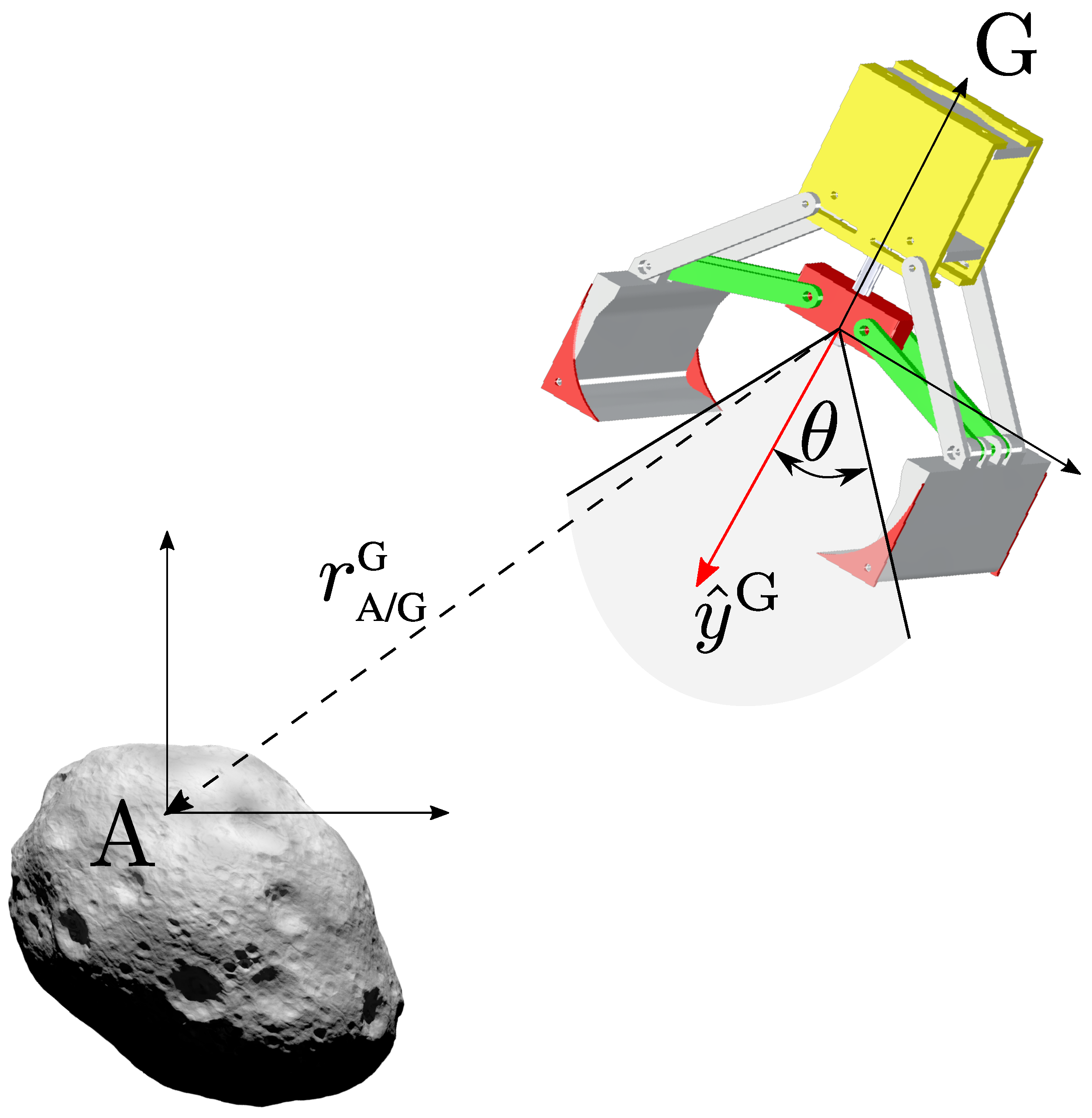
Proposition 1.

Consider the domain $\mathcal{D}=\{{\mathit{q}}_{\mathrm{G}/\mathrm{A}}\in {\mathbb{H}}_d:{\mathit{q}}_{\mathrm{G}/\mathrm{A}}\circ {\mathit{q}}_{\mathrm{G}/\mathrm{A}}\le 1+\frac{1}{4}{\delta }^2\}$. The line of sight constraint depicted in Figure 5 can be encoded as

$$r_{\mathrm{A}/\mathrm{G}}^{\mathrm{G}}·{\widehat{y}}^{\mathrm{G}}\ge \parallel r_{\mathrm{A}/\mathrm{G}}^{\mathrm{G}}\parallel cos\theta ,$$

(90)

and it requires that the angle between $r_{\mathrm{A}/\mathrm{G}}^{\mathrm{G}}$ and ${\widehat{y}}^{\mathrm{G}}$ remains less than θ. Using dual quaternions, this constraint can be equivalently expressed as

$$-{\mathit{q}}_{\mathrm{G}/\mathrm{A}}\circ (M_H\star {\mathit{q}}_{\mathrm{G}/\mathrm{A}})+2\parallel E_d{\mathit{q}}_{\mathrm{G}/\mathrm{A}}\parallel cos\theta \le 0,$$

(91)

where

$$M_H=\left[\begin{array}{cc}{0}_{4\times 4}& {⟦{\widehat{y}}^{\mathrm{G}}⟧}_{\mathrm{R}}^{\mathrm{T}}\\ {⟦{\widehat{y}}^{\mathrm{G}}⟧}_{\mathrm{R}}& 0_{4\times 4}\end{array}\right],$$

(92)

and it is convex over $\mathcal{D}$.

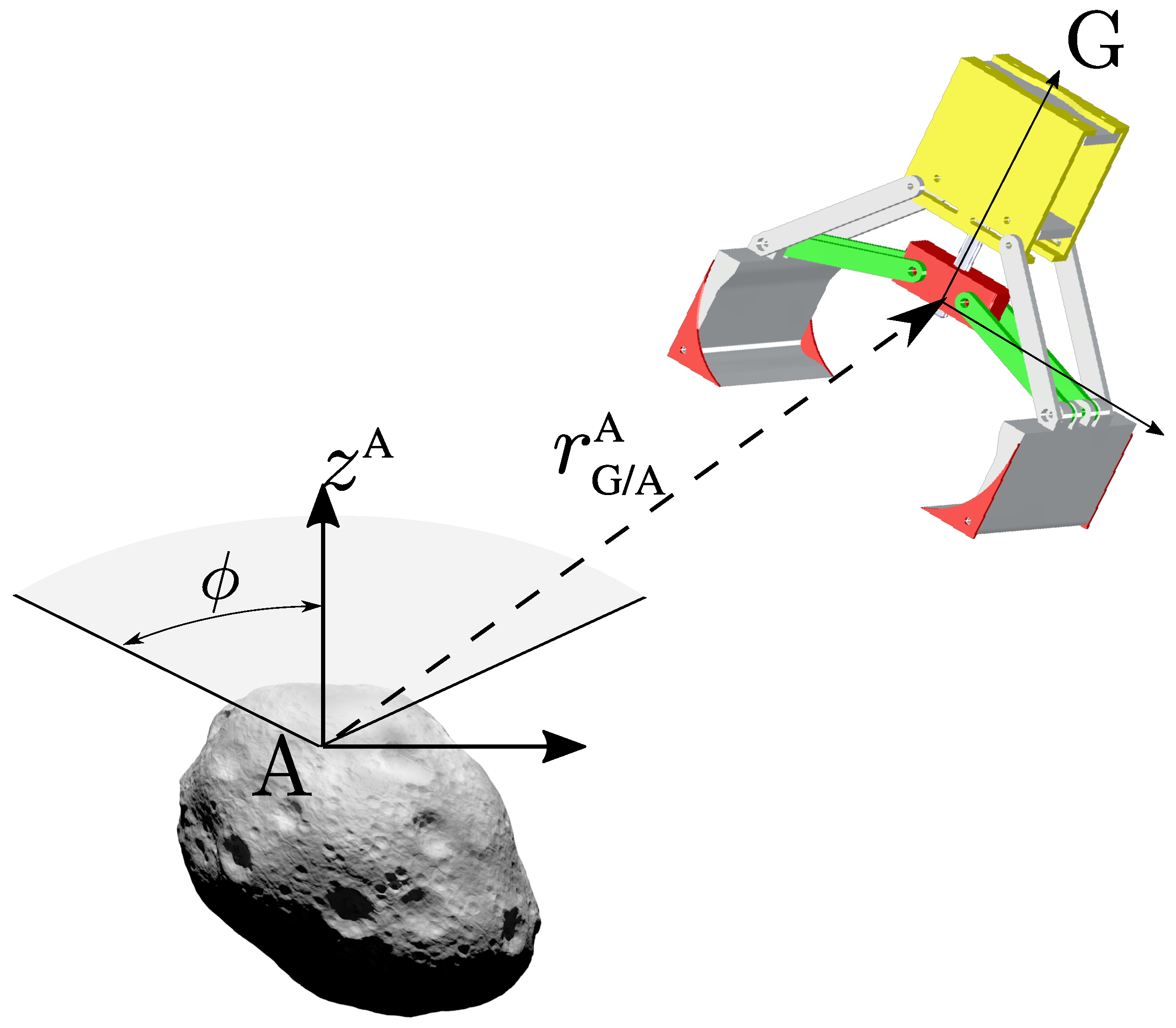
Proposition 2.

Consider the domain $\mathcal{D}=\{{\mathit{q}}_{\mathrm{G}/\mathrm{A}}\in {\mathbb{H}}_d:{\mathit{q}}_{\mathrm{G}/\mathrm{A}}\circ {\mathit{q}}_{\mathrm{G}/\mathrm{A}}\le 1+\frac{1}{4}{\delta }^2\}$. The approach slope constraint depicted in Figure 6, and the upper-and-lower bounded approach constraint depicted in Figure 7, can be encoded as

$$r_{\mathrm{G}/\mathrm{A}}^{\mathrm{A}}·{\widehat{z}}^{\mathrm{A}}\ge \parallel r_{\mathrm{G}/\mathrm{A}}^{\mathrm{A}}\parallel cos\varphi ,$$

(93)

and it requires that the angle between $r_{\mathrm{G}/\mathrm{A}}^{\mathrm{A}}$ and ${\widehat{z}}^{\mathrm{A}}$ remains less than ϕ. Using dual quaternions, this constraint can be equivalently expressed as

$$-{\mathit{q}}_{\mathrm{G}/\mathrm{A}}\circ (M_G\star {\mathit{q}}_{\mathrm{G}/\mathrm{A}})+2\parallel E_d{\mathit{q}}_{\mathrm{G}/\mathrm{A}}\parallel cos\varphi \le 0,$$

(94)

where

$$M_G=\left[\begin{array}{cc}{0}_{4\times 4}& {⟦{\widehat{z}}^{\mathrm{A}}⟧}_{\mathrm{L}}^{\mathrm{T}}\\ {⟦{\widehat{z}}^{\mathrm{A}}⟧}_{\mathrm{L}}& 0_{4\times 4}\end{array}\right],$$

(95)

and it is convex over $\mathcal{D}$.

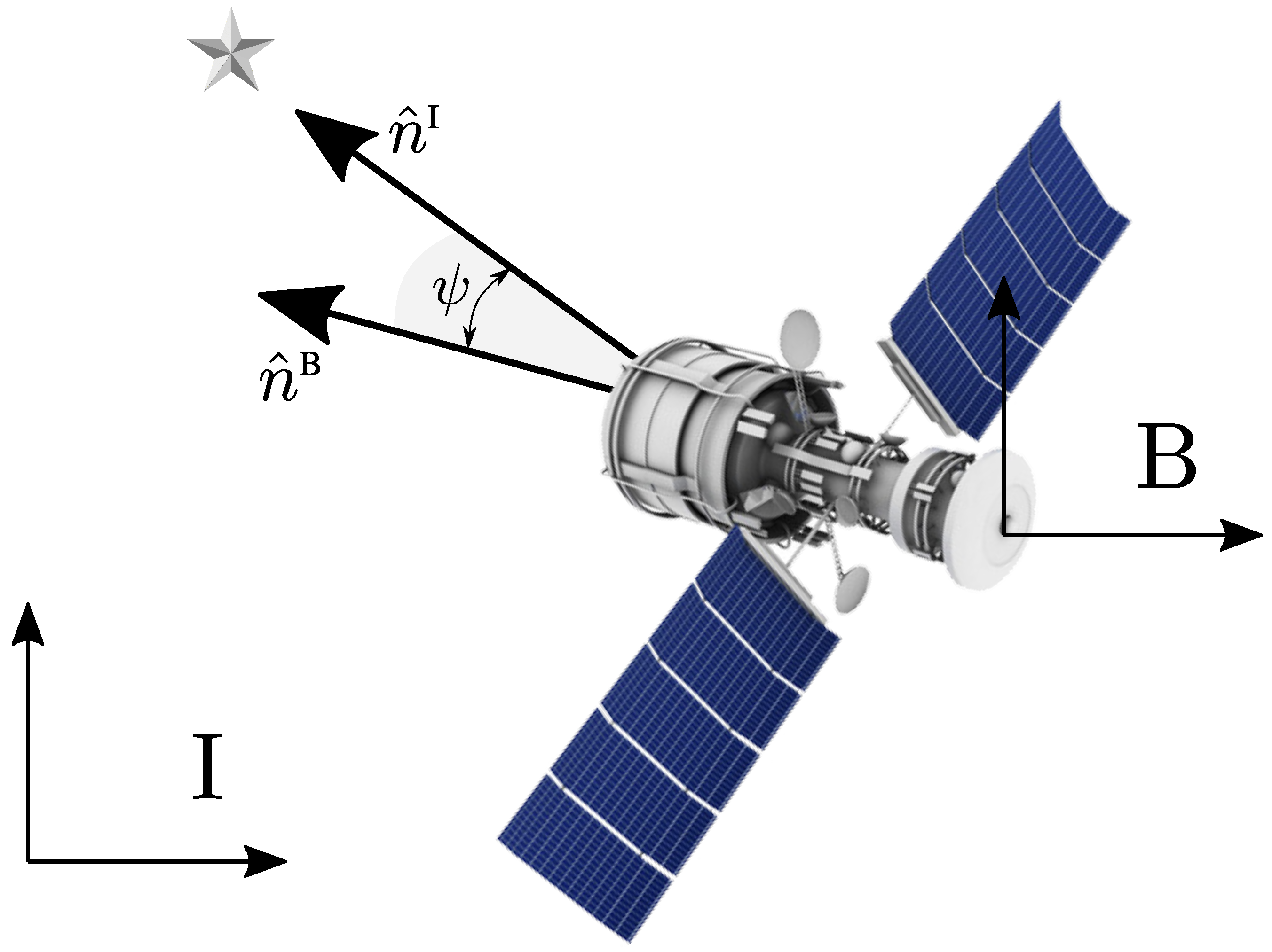
Proposition 3.

Consider the domain $\mathcal{D}=\{{\mathit{q}}_{\mathrm{B}/\mathrm{I}}\in {\mathbb{H}}_d:{\mathit{q}}_{\mathrm{B}/\mathrm{I}}\circ {\mathit{q}}_{\mathrm{B}/\mathrm{I}}\le 1+\frac{1}{4}{\delta }^2\}$. The attitude constraint depicted in Figure 8 can be encoded as

$${\widehat{n}}^{\mathrm{I}}·(q_{\mathrm{B}/\mathrm{I}}{\widehat{n}}^{\mathrm{B}}{q}_{\mathrm{B}/\mathrm{I}}^{*})\ge cos\psi ,$$

(96)

and it requires that the angle between the inertially fixed vector ${\widehat{n}}^{\mathrm{I}}$ and the body fixed vector ${\widehat{n}}^{\mathrm{B}}$ remains less than ψ. Using dual quaternions, this constraint can be equivalently expressed as

$${\mathit{q}}_{\mathrm{B}/\mathrm{I}}\circ (M_A\star {\mathit{q}}_{\mathrm{B}/\mathrm{I}})+cos\psi \le 0,$$

(97)

where

$$M_A=\left[\begin{array}{cc}{⟦{\widehat{z}}^{\mathrm{I}}⟧}_{\mathrm{L}}{⟦{\widehat{z}}^{\mathrm{B}}⟧}_{\mathrm{R}}& 0_{4\times 4}\\ 0_{4\times 4}& 0_{4\times 4}\end{array}\right],$$

(98)

and it is convex over $\mathcal{D}$.

6. Conclusions

In this paper we have explored the use of dual quaternions for robot modeling. In particular, the main contribution of this paper is a generalizable framework to capture the kinematics of spacecraft-mounted robotic manipulators using a dual quaternion approach. We took a bare-bones approach that built up to a convenient description of the end-effector’s dual velocity, making use of a more intuitive forward kinematics methodology than the existing methods in the literature. Previous works on robot kinematics using dual quaternions provided either strict geometry-dependent approaches or were only applicable to fixed-base robots. The work presented herein is highly relevant in combination with the latest literature in dynamic modeling of robot manipulators using dual quaternions. Additionally, in our study of kinematics, we developed a convenient and simple-to-implement representation of the body-frame Jacobian matrix. The proposed form of the Jacobian exploits a convenient matrix representation of the adjoint dual quaternion transformation so that, in combination with the newly proposed form of the screw matrix, it avoids the artificial separation of the contribution by the generalized speeds of a given joint. Finally, we have provided a summary, and re-interpretation, of several existing results on the topic of dual quaternions, emphasizing their applicability on spacecraft-mounted robots. These included results on the exponential and logarithmic maps, an exposition on the use of the DH parameters, and finally the casting of the dual quaternion representation of constraints (originally developed for EDL purposes) interpreted in the context of a gripper-target system on-board a spacecraft.

Future work in this area will aim at implementing kinematic control laws for end-effector pose control when the based is not fixed to an inertial reference frame. This should be possible by following the steps in Özgür and Mezouar [20], and through the use of the Generalized Jacobian Matrix [28].

References

- Reed, B.B.; Smith, R.C.; Naasz, B.J.; Pellegrino, J.F.; Bacon, C.E. The Restore-L Servicing Mission. AIAA Space Forum 2016. [Google Scholar] [CrossRef]
- NASA Goddard Space Flight Center. On-Orbit Satellite Servicing Study, Project Report. In National Aeronautics and Space Administration, Goddard Space Flight Center; Technical Report; NASA: Greenbelt, MD, USA, 2010. [Google Scholar]
- Saha, S.K.; Shah, S.V.; Nandihal, P.V. Evolution of the DeNOC-based dynamic modelling for multibody systems. Mech. Sci. 2013, 4, 1–20. [Google Scholar] [CrossRef] [Green Version]
- Todorov, E.; Erez, T.; Tassa, Y. MuJoCo: A physics engine for model-based control. In Proceedings of the 2012 IEEE/RSJ International Conference on Intelligent Robots and Systems, Vilamoura, Portugal, 7–12 October 2012. [Google Scholar]
- Featherstone, R. Rigid Body Dynamics Algorithms; Springer: Berlin/Heidelberg, Germany, 2008. [Google Scholar]
- Wang, J.; Liang, H.; Sun, Z.; Zhang, S.; Liu, M. Finite-Time Control for Spacecraft Formation with Dual-Number-Based Description. J. Guid. Control Dyn. 2012, 35, 950–962. [Google Scholar] [CrossRef]
- Filipe, N.; Tsiotras, P. Simultaneous Position and Attitude Control Without Linear and Angular Velocity Feedback Using Dual Quaternions. In Proceedings of the 2013 American Control Conference, Washington, DC, USA, 17–19 June 2013; pp. 4815–4820. [Google Scholar]
- Filipe, N.; Tsiotras, P. Rigid Body Motion Tracking Without Linear and Angular Velocity Feedback Using Dual Quaternions. In Proceedings of the European Control Conference, Zurich, Switzerland, 17–19 July 2013; pp. 329–334. [Google Scholar]
- Seo, D. Fast Adaptive Pose Tracking Control for Satellites via Dual Quaternion Upon Non-Certainty Equivalence Principle. Acta Astronaut. 2015, 115, 32–39. [Google Scholar] [CrossRef]
- Tsiotras, P.; Valverde, A. Dual Quaternions as a Tool for Modeling, Control, and Estimation for Spacecraft Robotic Servicing Missions. In Proceedings of the Texas A&M University/AAS John L. Junkins Astrodynamics Symposium, College Station, TX, USA, 20–21 May 2018. [Google Scholar]
- Valverde, A.; Tsiotras, P. Modeling of Spacecraft-Mounted Robot Dynamics and Control Using Dual Quaternions. In Proceedings of the 2018 American Control Conference, Milwaukee, WI, USA, 27–29 June 2018. [Google Scholar]
- Perez, A.; McCarthy, J. Dual Quaternion Synthesis of Constrained Robotic Systems. J. Mech. Des. 2004, 126, 425–435. [Google Scholar] [CrossRef] [Green Version]
- Perez, A. Dual Quaternion Synthesis of Constrained Robotic Systems. Ph.D. Thesis, University of California, Irvine, CA, USA, 2003. [Google Scholar]
- Pennestrì, E.; Stefanelli, R. Linear algebra and numerical algorithms using dual numbers. Multibody Syst. Dyn. 2007, 18, 323–344. [Google Scholar] [CrossRef] [Green Version]
- Radavelli, L.A.; De Pieri, E.R.; Martins, D.; Simoni, R. Points, Lines, Screws and Planes in Dual Quaternions Kinematics. In Advances in Robot Kinematics; Lenarcic, J., Khatib, O., Eds.; Springer: Berlin, Germany, 2014; pp. 285–293. [Google Scholar]
- Leclercq, G.; Lefèvre, P.; Blohm, G. 3-D Kinematics Using Dual Quaternions: Theory and Applications in Neuroscience. Front. Behav. Neurosci. 2013, 7, 1–7. [Google Scholar] [CrossRef] [PubMed]
- Quiroz-Omaña, J.J.; Adorno, B.V. Whole-Body Kinematic Control of Nonholonomic Mobile Manipulators Using Linear Programming. J. Intell. Robot. Syst. 2017, 91, 263–278. [Google Scholar] [CrossRef]
- Brodsky, V.; Shoham, M. Dual numbers representation of rigid body dynamics. Mech. Mach. Theory 1999, 34, 693–718. [Google Scholar] [CrossRef] [Green Version]
- Filipe, N. Nonlinear Pose Control and Estimation for Space Proximity Operations: An Approach Based on Dual Quaternions. Ph.D. Thesis, Georgia Institute of Technology, Atlanta, GA, USA, 2014. [Google Scholar]
- Özgür, E.; Mezouar, Y. Kinematic Modeling and Control of a Robot Arm Using Unit Dual Quaternions. Robot. Autom. Syst. 2016, 77, 66–73. [Google Scholar] [CrossRef]
- Filipe, N.; Tsiotras, P. Adaptive Position and Attitude-Tracking Controller for Satellite Proximity Operations Using Dual Quaternions. J. Guid. Control Dyn. 2014, 38, 566–577. [Google Scholar] [CrossRef]
- Bhat, S.; Bernstein, D. A topological obstruction to global asymptotic stabilization of rotational motion and the unwinding phenomenon. In Proceedings of the 1998 American Control Conference, Philadelphia, PA, USA, 26 June 1998. [Google Scholar] [CrossRef]
- Murray, R.M.; Li, Z.; Sastry, S.S. A Mathematical Introduction to Robotic Manipulation; CRC Press: Boca Raton, FL, USA, 1994. [Google Scholar]
- Jazar, R.N. Theory of Applied Robotics: Kinematics, Dynamics, and Control; Springer: Berlin, Germany, 2010. [Google Scholar]
- Gan, D.; Liao, Q.; Wei, S.; Dai, J.; Qiao, S. Dual Quaternion-Based Inverse Kinematics of the General Spatial 7R mechanism. Proc. Inst. Mech. Eng. C J. Mech. Eng. 2008, 222, 1593–1598. [Google Scholar] [CrossRef]
- Adorno, B.V. Two-Arm Manipulation: From Manipulators to Enhanced Human-Robot Collaboration. Ph.D. Thesis, Université Montpellier II Sciences et Techniques du Languedoc, Montpellier, France, 2011. [Google Scholar]
- Lee, U.; Mesbahi, M. Constrained Autonomous Precision Landing via Dual Quaternions and Model Predictive Control. J. Guid. Control Dyn. 2017, 40, 292–308. [Google Scholar] [CrossRef]
- Umetani, Y.; Yoshida, K. Resolved motion rate control of space manipulators with generalized Jacobian matrix. IEEE Trans. Robot. Autom. 1989, 5, 303–314. [Google Scholar] [CrossRef]
Figure 1.
Screw motion parametrized by and .
Figure 2.
Denavit-Hartenberg parameters.
Figure 3.
Robot arm configuration.
Figure 4.
Figure 5.
Line-of-sight constraint during grappling.
Figure 6.
Approach slope constraint.
Figure 7.
Upper-and-lower bounds constraint.
Figure 8.
General attitude constraint with respect to inertial directions.