URSIM: Unique Regions for Sketch Map Interpretation and Matching


School of Natural Science, University of Örebro, 70281 Örebro, Sweden
*
Author to whom correspondence should be addressed.
Robotics 2019, 8(2), 43; https://doi.org/10.3390/robotics8020043
Submission received: 3 April 2019
/
Revised: 31 May 2019
/
Accepted: 3 June 2019
/
Published: 5 June 2019
Abstract
:We present a method for matching sketch maps to a corresponding metric map, with the aim of later using the sketch as an intuitive interface for human–robot interactions. While sketch maps are not metrically accurate and many details, which are deemed unnecessary, are omitted, they represent the topology of the environment well and are typically accurate at key locations. Thus, for sketch map interpretation and matching, one cannot only rely on metric information. Our matching method first finds the most distinguishable, or unique, regions of two maps. The topology of the maps, the positions of the unique regions, and the size of all regions are used to build region descriptors. Finally, a sequential graph matching algorithm uses the region descriptors to find correspondences between regions of the sketch and metric maps. Our method obtained higher accuracy than both a state-of-the-art matching method for inaccurate map matching, and our previous work on the subject. The state of the art was unable to match sketch maps while our method performed only 10% worse than a human expert.
1. Introduction
In a time where touch screens are everywhere, from our laptops to our phones, drawing provides an intuitive and simple interface for human–robot interactions. As shown in the work of Blades [1], sketch maps are a reliable data acquisition tool to communicate information about an environment and to provide directions. However, sketch maps are abstract representation of the environment: they are not typically metrically accurate and may not include key information the user deemed unnecessary or forgot. Furthermore, the person drawing will use different strategies to make the map easy to understand, e.g., simplification of the representation by lowering the amount of details or accurate description of key places. However, as shown by Jan et al. [2], sketch maps correctly represent the topology of the environment and provide a relatively accurate representation at key locations. In a scenario where a sketch map is used as a tool to give directions toward a goal, an important place such as a crossing might be drawn as accurately as possible to avoid navigation errors. On the other hand, corridors are easy to navigate and will not necessitate the same attention to details. Hence, a user following indications on a sketch map can easily navigate corridors and reach points of interest, even when the representation of the corridors in the sketch map is inaccurate.
Understanding a sketch map depends on three abilities: the ability to understand the topology of the map, the ability to identify each individual element, such as rooms, corridors, and crossings, and the ability to evaluate their importance. While simplifying the representation, and changing the level of details in the sketch map might make it easier for a human to understand the map, it adds in complexity for the robot. Looking at Figure 1, one can see a metric map of an indoor environment (Figure 1a) and four associated sketch maps. Interpreting the sketch maps is not trivial: Figure 1b is missing a corridor, in Figure 1d the middle corridor is not present in the metric map, and all maps have large structural errors and errors in local scale, i.e., it is impossible to use a single transformation to align the sketch and metric maps. Hence, a robot using a sketch map as an interface needs to solve the hard problem of matching a semi-abstract representation with its own map of the environment.
While finding correspondences between elements of a sketch map and a metric map is a complex problem, the use for such a method is there: once the robot is able to match sketch maps to its own metric map, sending navigation commands can be as simple as starting one’s phone, sketching the environment, and directing the robot to its goal. In our work, we try to answer the question of how to find correspondences between equivalent elements of a sketch map and an equivalent metric map.
2. Method Outline and Contributions
We present the Unique Regions for Sketch map Interpretation and Matching (URSIM) method to find element-wise correspondences between a sketch map and an equivalent metric map representing the environment. URSIM takes as inputs two maps segmented in regions and finds the most distinguishable, or unique, regions in each map.
We call such regions anchors. Both segmented maps are then converted to graphs where each region is a vertex and we have an edge between each region in contact. A vertex descriptor is created for each vertex based on the topology of the map, the position of anchors, and the size of regions. Finally, using a planar graph matching algorithm, URSIM finds the most likely correspondences between both graphs’ vertices.
An illustration of the method can be seen in Figure 2.
The contributions of this paper are:
- A method to determine unique regions in segmented maps is proposed. By comparing the characteristics of each segmented region to other regions of the same map, we determine the most distinguishable, or unique, regions.
- A method to find two sets of equal length containing the most similar unique regions between two maps is presented. The unique regions in those sets are called anchors and are used later during the matching.
- A vertex descriptor using anchors in a graph with weighted vertices to compare the regions of two maps is introduced. Each vertex descriptor represents the topology of the environment around said vertex, relative to the position of anchors in the graph and the size of all other regions.
- An improvement of the graph matching algorithm used in our previous work [3] was confirmed. Instead of using a specific characteristic, such as a region being a crossing or a dead end, we changed the similarity measure used to compare vertices and compare the vertex descriptors presented in the previous point. A user–chosen similarity threshold determines when vertices are similar enough to be matched together.
3. Related Work
Few methods have been developed to match maps with a high level of abstraction. Instead, most works focus on matching partial metric maps or limit the extent to which maps can differ by using particular types of maps such as CAD models, aerial images, or blueprint layouts [4,5,6,7,8]. It is easy to understand why that is: similar maps can use easily describable similarity measures based on direct sensor measurements or some classic descriptors such as SIFT.
On the other hand, sketch maps have a high level of abstraction in the representation and one needs to understand their implicit characteristics, such as their topology, to be able to use them: a matching method that depends on correct metric information will lead to incorrect correspondences when used on sketch maps.
However, sketch maps are used to convey information about the world and, thus, while they are abstract representations of an environment, there is still a logic to how they are related to the real world. That logic is conveyed through the topology of the environment and by putting emphasis on accurate representation of important information; important information being decided in a subjective manner by the person drawing.
A common way to find the topology of a map is to use its Voronoi diagram. The Voronoi diagram is the set of all points at equal distance from at least two obstacles, and, as such, represents the topology of the environment through its skeleton [9,10]. Working on metric maps with errors due to drift or sensor noise, Schwertfeger and Birk [11,12] evaluated map quality by matching topology graphs derived from the Voronoi diagrams of two grid maps. They used the wavefront propagation algorithm to find a matching between the graphs. Correspondences are determined based on a similarity measure between vertices and ICP [13] using the local maps around the vertices. They tested their method on maps obtained by multiple robots during the RoboCup Rescue. While their method leads to good matching results on sensor maps, it did not work well with sketch maps due to the multiple parameters that needed tuning on a per map basis [3]. In this article, we propose to use a different similarity measure that needs less parameters and is more robust to large differences in scale or representation between the maps.
Park et al. [14] merged maps using rectangular features to estimate the largest shared area. They assumed that the environment was made of polygons with orthogonal angles. Their method is able to handle rotations and different global scales but cannot handle deformations of the map. While the idea of segmenting the map into similar regions for matching is also used in URSIM, URSIM is more robust to local changes.
Some works use CAD maps representing a building in a metrically correct way. For example, Boniardi et al. [8] presented a method for localization using a CAD floor plan as prior map. They performed matching between maps from different modalities by using maximum a posteriori pose-graph-based SLAM system [15]. They reported better localization results than Monte-Carlo localization on seven datasets. Although the method can handle some clutter in the environment, the paper states that “significant or even full occlusion due to clutter or large installations have a substantial effect on the method”. It should be also noted that associations can be hard to find between maps with a high level of disparity and performing pose graph optimization using sensor measurements might be impossible if the map built by the robot and the sketch differ too much. On the other hand, our method is able to find correspondences between maps with large structural differences.
Kakuma et al. [7] aligned an occupancy grid map with a floor map to obtain semantic information about the environment. They segmented the environment using morphological operations and created a graph out of the segmentation. Using the shape of each region, they aligned the graph of the occupancy map and the floor map using graph matching [16] and a similarity transform matrix computed from correspondences of the regions. They tested their method in two environments and obtained an error rate in scale, rotation, and translation of less than compared to the alignment given by a user. However, their method needs both maps to have similarly shaped regions after segmentation since the region comparison is based on the Hu moments. Thus, URSIM can handle maps with higher disparity than their method.
Freksa et al. [5] used schematic maps for interaction between a human and a robot, and between a robot and its environment. A schematic map corresponds to a user–provided map depicting a simplified version of the topology of the environment.
Corner correspondences between the environment and the schematic map are found by mapping features detected in sensor space to features in the schematic map.
They tested their method on a simulated environment with three rooms. By definition, their matching method depends on the ability to find spatial features and, since those features are not always present in sketch maps, our method does not rely on them for matching. In addition, in the work of Freksa et al. [5], correct interpretation of the spatial relationships is only possible because the schematic map creation step is highly restricted, e.g., walls need to be straight and features easy to detect. On the other hand, our method handles high disparity between the maps and is less restrictive about the way the input is supposed to be drawn.
Setalaphruk et al. [4] studied navigation in an indoor environment using a map provided by a user as input. They used the crossings and dead-ends of the Voronoi diagram as landmarks. While correct corridor length was not needed, the walls in the map had to be straight and the existence and connectivity of corridors had to be correct. Hence, their method assumes a sufficiently accurate representation of the environment. Our method is able to match regions of two maps almost independently of local scaling and does not require a metrically accurate representation.
Gholami Shahbandi et al. [17] developed a method to align a user given layout map and a sensor-built map. A layout map is defined as a simplified representation of a building that can have errors in local scaling and representation. As such, compared to other related works, the work of Gholami Shahbandi et al. [17] is the most similar to ours in terms of its aim and the types of map used. However, their alignment method is based on finding features such as walls and corners, which is not easy to achieve on sketch maps. We evaluate the performance of URSIM compared to the method of Gholami Shahbandi et al. [17] in Section 6.5.
Shah and Campbell [18] performed navigation using a sketch map of obstacles provided by the user. They extracted waypoints from the Voronoi diagram and estimated the transformation between the sketch map and the environment using a weighted least square affine matrix. The sketches were scaled and rotated to fit the environment, and errors in local scale and representation were handled by the path planner. However, obstacles and landmarks are not always represented in maps and our method handles that case.
Chronis and Skubic [19,20], Parekh et al. [21], and Skubic et al. [22,23] developed a sketch-map interface for robot control on a PDA and used it for navigation of one or a team of robots in an indoor environment. They conducted a usability study which gave an average rating of 4.2 on a Likert scale [24] to the sketch interface, with 5 being the maximum, showing that sketch maps are an intuitive interface. However, for all methods, the correspondences between the sketch interface and the map of the environment are found using isolated objects described by histograms of forces. Our method does not need isolated objects and landmarks to find correspondences between the maps.
In our previous work [3], we matched hand-drawn sketch maps to a ground truth map using the Voronoi diagram trimmed down automatically using the free space in the map. We used that diagram as a graph and performed planar graph matching. We obtained a rate of correct correspondences between vertices of on a simple environment, and of on a real environment. However, we found that using the Voronoi diagram to find correspondences sketch maps is not sufficient due to the pronounced differences between sketch and ground truth maps. The method presented in this article segments the map in regions, and thus removes the need to use the Voronoi diagram, leading to more correct correspondences as shown in Section 6.2.
In conclusion, no method in the state of the art is suitable for matching sketch maps to metric maps. Indeed, all methods presented above have assumptions about prior maps, such as metric accuracy or the presence of specific features in the maps, and those assumptions are not realistic for sketch maps. Hence, the related work cannot take into account the local scaling errors and differences in representation, or in the level of detail, between a sketch map and an equivalent metric map. On the other hand, our method can find correspondences between sketch maps with large differences in detail or representation compared to an equivalent metric map, with only two assumptions about the sketch map: that it is clutter free, and that it represents the walls of the environment.
4. Segmenting the Maps and Building the Anchor Sets
Sketch maps of indoor places cannot directly be used as metric maps due to errors in local scale, non-homogeneous levels of detail, and the approximation of distances and sizes. Instead of using a sketch map as an accurate representation of an environment, a person using a sketch map will focus on the topology and points of interest along the trajectory [25], i.e., places that are distinct from the rest of the environment. However, as demonstrated by Mielle et al. [3], using the topology of the environment alone is not enough to find correspondences between sketch and metric maps. Indeed, sketch maps can vary greatly from the metric map and, while the topology of both the sketch and the metric map can be correct, the schematization of the sketch can make it hard to find correct correspondences due to the difference in the level of detail. In our previous work [3], we extracted the topology by computing the Voronoi Diagram of the maps and used a planar graph matching algorithm to find correspondences between the diagrams. We obtained a matching accuracy of 58% on a dataset of sketches and we came to the conclusion that to get better correspondences between a sketch and an equivalent metric map, we would need to consider more than just the topology of the environment represented by the Voronoi diagram.
URSIM takes a different approach. URSIM takes as inputs the sketch and metric maps, segmented into regions using a given map segmentation algorithm (see Section 4.1), and finds the most unique regions in each map, as presented in Section 4.2 and Section 4.3. Section 5.1 presents how URSIM then builds region descriptors using those unique regions, the topology of the map, and attributes of the regions. Finally, correspondences between the regions are found using graph matching, as described in Section 5.2.
4.1. Map Segmentation
For segmentation of the sketch and metric maps, we use the MAORIS [26] algorithm. MAORIS’ main advantage is its ability to segment maps from different modalities in a way similar to that of a human, reducing errors due to differences of representation or level of detail.
When segmenting the maps, the first step of the MAORIS algorithm changes each pixel’s value to the diameter of the largest circle that can be fitted in free space and contains the respective pixel. Then, pixels with the same values are merged into regions. Noise in the segmentation is removed by detecting and merging special regions called ripples. Finally, neighboring regions with similar values are merged together. For a more detailed description of the MAORIS algorithm, we refer the reader to the corresponding paper [26].
It should be noted that other segmentation methods, such as Voronoi segmentation [27] or DuDe [28], could be used as well in URSIM. However, since MAORIS was developed for maps from different modalities and returned more accurate segmentation results than previous state-of-the-art segmentation methods [27,28] on a dataset of sketch and metric maps, all maps in our work were segmented using MAORIS.
4.2. Finding Unique Regions in a Segmented Map
Given a set of regions from a segmented map, the first step of the URSIM method is to find the most unique regions, i.e., the most distinguishable ones. To do so, each region is associated with a set of N attributes with values , with , representing different characteristics such as the size or shape of each region. All attributes are standardized to have comparable values and avoid the effect of outliers. While normalizing would reduce the differences between in the presence of outliers, standardizing, which gives the data a mean of 0 and a standard deviation of 1, mitigates the effect of outliers. Using the set of all attributes i for a given map, the set is standardized using the standard score:
with being the mean of all regions’ and being the standard deviation. If the value of any of a region is at least 1 standard deviation away from the mean, we consider the region’s attribute, and thus the region, to be unique.
In our method, we use two simple attributes based on the way MAORIS uses free space to segment maps: the size of each region and their general shape. The size of a region corresponds to the number of pixels in it. The shape of a region is roughly estimated by using the eigenvalues of its two first principal components (PC): more circular regions will have similar eigenvalues, while elongated regions will have different eigenvalues. To obtain a scalar parameter from the PCs describing the shape of a region, we first calculate the eigenvalues of the two first PCs. We then normalize the eigenvalues between 0 and 1 by dividing both of them by the larger one. Finally, the attribute representing the shape is the difference between both normalized eigenvalues. An example of unique regions in a sketch map is shown in Figure 3. However, it should be noted that the method to find unique regions is independent of the set of attributes used. One could use different attributes depending on the type of map or segmentation. We left the study of additional suitable attributes for future work.
4.3. Creating the Sets of Anchors from the Unique Regions of the Sketch and Metric Maps
Given a sketch and metric map, the number of unique regions found in each map might be very different, e.g., if one map has multiple similar looking regions compared to the other map, or if a map represents a bigger part of the environment than the other. As presented in Section 5.1, the URSIM method uses the position of all unique regions to build region descriptors representing the topology of the environment and the position of the anchors. Hence, having a different number of unique regions between the sketch and metric maps may create dissimilar region descriptors between otherwise equivalent regions. In this section, we present how, before creating the region descriptors, URSIM reduces both sets of unique regions to the same length by finding the most similar unique regions between the sketch and metric maps.
We define the disparity score d between two regions R and R’ as the mean of the differences of their attributes standardized:
and use the Hungarian matching algorithm [29], with weights given by the disparity score, to find the set of unique regions that are the most similar.
In practice, the Hungarian algorithm finds correspondences between the two sets of unique regions, effectively making both sets of unique regions equal in length if we disregard the regions that were not matched. However, since the topology of the environment is not yet taken into account, the correspondences are often not correct, as can be seen in Figure 4. Thus, this step is only used to reduce the sets of unique regions to two sets of equal length by removing the most dissimilar unique regions between the maps, i.e., the regions unmatched by the Hungarian matching. However, the Hungarian matching correspondences themselves are not used in the rest of the method.
We refer to the regions in the reduced sets as the anchors of the maps.
5. Graph Matching
5.1. Computing Vertex Descriptors that Express Topological Similarity with Respect to the Anchors and the Standardized Size of Regions
After reducing the set of unique regions as described in Section 4.3, we have two sets of equal length containing the most similar unique regions between the maps, i.e., the anchors. However, those anchors typically only concern a subset of all regions in the environment. The remaining regions not included in the anchor sets do not have attributes that distinguish them from most of the other regions in the map. To be able to express the similarity between all regions, and not just the anchors, the next step of the URSIM method creates region descriptors for all regions in both the sketch map and the metric map.
From a segmented map, we build a graph where each vertex corresponds to a region and edges connect regions in contact. The graph creation process is illustrated in Figure 5. We then compute a descriptor for each vertex. We built on the Laplacian Family Signature (LFS) presented by Hu and Guibas [30]. The LFS of a vertex with index u is the vertex descriptor describing a given vertex’s structural relationship to its extended neighborhood:
The expression of the LFS depends on the eigenpairs of the graph Laplacian with representing the uth element of the eigenvector k, and where is a real-valued function. The calculation of depends on the uth elements of due to the ordering of the vertices used when calculating . While the calculation of the graph Laplacian is described in more detail below, it should be noted that is a matrix representation of the graph. More precisely, measures the extent to which a graph differs at one vertex from its values at nearby vertices. Given a graph with V vertices, the vertices are ordered from to to calculate as follow:
where relates vertex n to vertex m. When calculating the eigenpairs of , a given vertex is directly related to the element u of each eigenvector k, according to the ordering used to calculate . For a given eigenvector , we have:
where relates to .
In our work, we use the heat kernel signature (HKS) as the real-valued function . The HKS was presented by Aubry et al. [31] and represents the relationship of a given vertex to its neighborhood in terms of simulated heat diffusion. For each vertex, the signature records the amount of heat left at the vertex at a number of times assuming a unit amount of heat is put on the vertex initially. The HKS for each vertex is expressed as and is intrinsic, meaning that, if two graphs are isomorphic, then the signatures of corresponding vertices are the same, i.e., equivalent vertices dissipate heat similarly. The signatures are also stable under small perturbations [30]. Hence, the similarity between two vertices can be evaluated by comparing their HKS.
However, for each vertex, the heat diffusion should be influenced by the size of the region. As in a real environment, a smaller room should diffuse heat to neighboring rooms faster than a larger room. Without taking the size of a region into account, every vertex will diffuse heat in the same way and important information given by the segmentation will be lost during the matching. Thus, each vertex is associated with a weight corresponding to the standardized size attribute of the corresponding region, as illustrated in Figure 5. We use the standardized size of regions to reduce scaling errors between the sketch and metric maps. However, the graph Laplacian used by Hu and Guibas [30] for the LFS is expressed with weights on the edges instead of the vertices. Indeed, the generalized graph Laplacian is defined as the difference between the diagonal matrix of the vertex degree and is the graph adjacency matrix:
with the set of edges in the graph and w the weights on the edges, i.e., .
where vertex v has weight and means that the vertex u and v are adjacent.
To express the graph Laplacian, and by extension the LFS, with weights on the vertices instead, we use the formulation proposed by Chung and Langlands [32].
To be able to use the graph Laplacian defined in Equation (7) to find the eigenvectors and values of the graph, which are necessary for the LFS, one needs to prove that is symmetric and positive semi-definite. Since this aspect of was not shown by Chung and Langlands [32], we show that is indeed symmetric and positive semi-definite. We can define the incidence matrix as in the work of Chung and Langlands [32]:
Thus, we have . If we consider the eigen decomposition of with unit-norm eigenvector and corresponding eigenvalue , we have:
Since can be written as the inner product of the vector with itself, this shows that and so the eigenvalues of are all non-negative and is positive-semidefinite, allowing us to use the eigenvectors and eigenvalues of .
The LFS in Equation (3) represents the structural relationship of a vertex compared to its neighbors. Instead, we want the LFS to represent the structural relationship of the vertex compared to the set of anchors found in Section 4.2 and Section 4.3. Thus, we use the heat kernel value of anchor vertices at a given vertex, as presented by Hu et al. [33]. Namely, for any vertex v of a graph , we define the heat kernel distance to anchor vertices as:
with the set of anchor vertices. Equation (10) is equivalent to Equation (3) but restricted to anchors instead of expressed for all vertices in the graph. Hence, for a vertex u, instead of calculating the square of the uth element of the eigenvector k, we use the product of the uth element of eigenvector k, i.e., , with the element of eigenvector k corresponding to the anchor a, i.e., . Hence, Equation (10) describes the structural relationship of a vertex compared to its neighbors and the positions of all anchors in the graph, instead of the position of the vertex u itself.
5.2. Planar Graph Matching Using the Laplacian Family Signature
We extend the planar graph matching method presented in our previous work [3] to use the LFS. Our solution to the graph matching problem is a neighbor expanding matching strategy. To initialize the matching process, the matching algorithm starts by finding a set of pairs of vertices, also called seeds, between a graph G and a corresponding graph . How to find the seeds is described below. From each seed, the algorithm finds the correspondences between the vertices of their neighborhoods by considering all permutations of ordered neighbors and keeping the one that yields the minimum normalized Levenshtein edit distance [34]. The Levenshtein edit distance is the minimum number of single edits between two sequences required to change one sequence into the other. Given two vertices’ neighborhoods, we consider as possible changes: removing a vertex and all of its edges, adding a vertex and an edge, or replacing a vertex. Each removal, replacement, or vertex creation is one edit. Thus, removing a vertex and all its edges has a cost of with n the number of edges associated with the vertex. On the other hand, adding a vertex and an edge has a cost of 2 and replacing a vertex a cost of 1. Then, to find all correspondences between vertices of the graphs, the neighborhood matching process is repeated for newly obtained vertex-to-vertex correspondences until no correspondence is left to expand.Once all seeds have been expanded, the final solution to the matching problem is the one with the lowest cost when adding both the cost of all correspondences and the cost of removing, in both graphs, all vertices without a correspondence, and their associated edges. See Algorithm 1 for the pseudocode of the matching algorithm and Figure 6 for an illustration of the calculation of the Levenshtein edit distance between two neighbors.
| Algorithm 1: Graph-Edit-Distance matching algorithm. |
 |
To decide when to remove or replace a vertex, the Levenshtein edit distance needs a comparison measure between vertices. We define the comparison measure between two vertices as the mean absolute difference between their heat kernel anchor distances over times samples, starting from 0 and with a sampling time of n:
where u is a vertex of the graph G and a vertex of . Since is bounded between 0 and 1, Equation (11) is also bounded between 0 and 1. The vertices are replaced or removed only if they are sufficiently different from each other up to a certain threshold m, i.e., . Stability to the threshold m is evaluated in Section 6.4. Similarly, we find the seeds by calculating for every possible correspondence between the vertices of G and . If , we create a new seed for the matching algorithm.
In the worst case with two graphs with p and y vertices, respectively, the algorithm would be and return possible solutions. However, since the heat diffusion is not usually the same in each graph, we observed during the experiments presented in Section 6 that the algorithm used of all possible seed combinations on average. Furthermore, in the same experiments, URSIM took on average less than s to find the correspondences between sketch and metric maps, even though the research code had not been optimized.
6. Experiments
We evaluated our dataset on 25 sketches presented in our previous work [26] and available online [35].
The sketch map dataset corresponds to the ground truth of the KTH dataset for SLAM (http://www.nada.kth.se/%7Ejohnf/kthdata/dataset.html). Twenty-five anonymous users explored a 3D environment online (http://mro.oru.se/wp-content/material/sketchmap-web/) and were asked to draw a 2D map from memory. The metric map representing the environment and four sketch maps are shown in Figure 1.
The correct correspondences, i.e., ground truth correspondences, between each sketch map and the metric map were manually annotated by both an expert in mobile robotics and an architect.
Given two segmented maps, the ground truth correspondences annotate which regions are equivalent. However, due to factors such as map resolution, level of detail, or noise in the measurements, the segmentation of the sketch and metric maps can differ and regions in the sketch map can be matched to more than one region in the metric map. Similarly, regions in the metric map can be matched to multiple regions in the sketch map, as illustrated in Figure 7.
We refer to such groups of correspondences as ground truth cliques.
We evaluated the set of correspondences returned by URSIM by calculating its score:
with the precision p:
and the recall r:
The score ranges between 0 and 1, with 0 being the worst possible score and 1 being the best. The precision and recall are calculated using the number of true positives , false positives , and false negatives . Given a set of correspondences between a sketch map and a metric map, true positives are correspondences where both vertices are present in the same ground truth clique. False positives are all correspondences for which both vertices are not present in the same ground truth clique. Finally, false negatives are all ground truth cliques for which no correspondence in the set corresponds to a true positive.
All results reported in this section were calculated over both ground truth sets.
6.1. Stability with Respect to the Number of Time Samples
Two intrinsic parameters of URSIM, present in Equation (11), are the sampling rate n used to calculate the values of t, and the number of samples . While the sampling rate n is closely related to the scale of the global information, there is no direct way to choose it. We investigated the stability of URSIM to those parameters by using between and time samples, and increasing by between subsequent samples. For each map and value of , the matching algorithm was run with different values of m, the threshold under which two vertices are considered similar, ranging from 0 to 1 by steps of . The highest score over all possible m was kept as the final matching score. The stability of URSIM to the threshold m is presented in Section 6.4.
Over the sketch map dataset, the scores obtained are fairly independent on , as shown in Figure 8. While using more time samples leads to slightly better results, the mean score is always above and stays fairly stable when using more than 10 time samples. Hence, while the value of the threshold m matters, as shown in Section 6.4, the number of time samples does not have much influence on the matching accuracy. Accordingly, in the rest of the experiments, we used a sampling rate and used .
6.2. Evaluation of the Scores
We calculated the scores over the sketch dataset using URSIM and evaluated the correspondences in terms of both the mean and median scores. While the mean enabled us to evaluate the general quality of the correspondences, the median gave a measure that disregards potential outliers. For example, a high median with a low mean value shows that, while most correspondences are correct, some incorrect correspondences returned low scores. On the other hand, a high mean with a low median means that most correspondences were wrong but correct ones scored very high. An efficient matching algorithm should have both mean and median as high as possible. As for the previous experiment, the matching algorithm was run with different values of m ranging from 0 to 1 by steps of , and the highest score over all possible m was kept as the final matching score.
As a baseline, we used the graph description proposed in our previous work [3] where regions are matched depending on their type: regions can either be crossings when they have more than one edge or dead-ends when they only have one edge. The results of the baseline are presented in the first column of Table 1. Furthermore, to test the effectiveness of URSIM’s graph matching method presented in Section 5.2, we replaced it by two different matching algorithms, the Hungarian matching and the VF2 algorithm developed by Cordella et al. [36], and compared their respective scores. While URSIM’s planar matching algorithm expands correspondences between vertices one neighborhood at the time, the Hungarian algorithm finds the solution of the assignment problem between the vertices. On the other hand, VF2 was developed to quickly find the largest common sub-graph between two large graphs. We also incrementally tested the usefulness of each attribute used to create the region descriptors by progressively building the descriptors and calculating the matching accuracy at each step. The second column of Table 1 presents the scores obtained when using only the topology to build the descriptors: anchors and weights on the vertices were not used to calculate the LFS. We refer to this test as and the flowchart of the algorithm can be seen in Figure 9a. The third column presents the test whose flowchart is illustrated in Figure 9b. For , the topology and positions of anchors in the graph were taken into account when calculating the LFS. However, vertices had equal weights and, thus, the relative sizes of regions were not taken into account. The fourth column shows the matching results of the test , where, when calculating the LFS, the weights on the vertices were the standardized region’s sizes but the positions of anchors in the graph were not taken into account (see Figure 9c). Finally, test , in the last column, corresponds to the full graph representation used by the URSIM method and used the topology, the positions of anchors in the graph, and the standardized size as weights for the vertices when calculating the LFS (see Figure 9d).
In all cases, the planar matching scored higher than both VF2 and the Hungarian matching. This result highlights the importance of using the topology as much as possible during the matching. Indeed, both the Hungarian matching and VF2 only consider the topology through the region descriptors. On the other hand, the planar matching presented in Section 5.2 starts from a pair of vertices, i.e., the seed, and expands the correspondences one neighborhood at a time, sequentially (see Line 10 of Algorithm 1). Therefore, the topology is taken into account both through the descriptors and by the planar graph matching algorithm during the neighborhood matching step.
Looking at the results of the planar matching in Table 1, URSIM has higher scores than the method presented in our previous work [3]. Furthermore, URSIM has the highest median and mean scores, with and , respectively, and, removing any attribute of the calculation of the LFS, leads to lower mean and median scores. Thus, we conclude that every attribute used in URSIM to build the descriptors and find correspondences is needed.
As a reference, we also calculated the median and mean scores between both sets of ground truth correspondences given by the users. While one set of ground truth correspondences was used in place of the correspondences returned by a matching algorithm, the other set was used as the ground truth set. One could expect the results for humans to be close to the maximum score, 1. However, the mean score is and the median is , showing that finding correspondences between a sketch map and a metric representation is not a trivial task, even for humans. The high level of abstraction and error in local scales, as shown in Figure 1 and mentioned in Section 3, make matching sketch maps a challenge even for humans.
6.3. Evaluation of the Scores over a Dataset of Partial Sensor Maps
To test the limits of the algorithm, we also applied URSIM to a scenario other than sketch-to-metric map matching: partially overlapping sensor maps built by one or more robots. We evaluated the accuracy of the correspondences on a dataset of 14 indoor sensor maps (https://github.com/saeedghsh/Halmstad-Robot-Maps) provided by Gholami Shahbandi et al. [17]. The dataset of indoor maps is composed of multiple partial views of an indoor environment scanned by a robot using a Google Tango tablet. Since the maps were built at different times and over different trajectories, they have different noise levels and cover different sets of rooms. As such, while the maps are largely metrically correct, the missing information between the maps make this dataset a challenge for matching algorithms. As for the sketch map dataset, the correct correspondences were manually annotated by both an expert in mobile robotics and an architect. However, while an actual metric map of the full environment was available for the sketch map dataset, this was not the case for the robot map dataset since the whole environment was never covered in one mapping run and every partial sensor map is, by definition, metric. Hence, since no partial sensor map is inherently a better metric map than the others for URSIM, each user created ground truth correspondences using a given partial sensor map as URSIM’s metric map. Both sensor maps used as URSIM’s metric maps are visible in Figure 10. We then ran the same tests with the same conditions as in Section 6.2.
Looking at the results in Table 2, one can see that again the planar matching algorithm scores higher than both the Hungarian matching and VF2. The planar algorithm outperforms Hungarian matching by for the median and by for the mean. Furthermore, VF2 did not manage to find any correct correspondence between the partial robot maps since the differences between the map’s graphs were too large. Looking at the results of URSIM, the scores are better than in our previous work [3]. However, URSIM was not designed for partial sensor maps: the median only increases significantly when using the anchors to build the descriptors while the mean stays the same with or without using the anchors. On the other hand, using the standardized size of regions decreased the matching accuracy. It should be noted that, even though using the anchors to create the region descriptors is the best strategy for partial sensor maps, worst-case matches got a lower score; only the median increased while the mean stayed stable. Hence, while using the LFS and anchors for matching sensor maps is better than the strategy used in our previous work [3], URSIM is not an ideal choice for finding correspondences between partial sensor maps.
6.4. Stability with Respect to the Threshold m
The planar matching depends on a parameter m, presented in Section 5.2, representing the threshold under which two vertices are considered similar. When looking at Figure 11, one can see that, for the previous experiment, the best m values are under for the sketch map dataset and under for the partial map dataset.
We evaluated how stable URSIM’s accuracy is with respect to the selection of the parameter m by calculating the scores with a fixed m value, for all maps in the datasets. We tested values of m ranging from to with a step size of . While the threshold m can vary between 0 and 1, we found that above the scores stayed constant and thus we only present the results between and . The stability is evaluated by looking at the median and mean of the scores.
In Figure 12, one can see a box plot of the scores over the sketch map dataset for fixed values of m. While both maximum median and mean are for , with the maximum median being and the maximum mean , the mean and median scores using a fixed m are significantly lower than the median and mean scores when choosing m on a per-map basis (see Section 6.2).
Hence, while for all sketch maps the best m value is under , using a fixed m value over the whole sketch map dataset leads to poorer matching results.
In Figure 13, one can see the same box plot as in Figure 12 over the partial map dataset. The region descriptors were built using only the topology and the position of anchors in the graph (see Figure 9b), since this strategy returned the highest scores on the partial sensor map dataset, as shown in Section 6.3. As for the sketch map dataset, using a fixed m value gives less accurate results than fine tuning the value of m for each map: a fixed value of m gives fairly stable results between and , however, it is constantly under the scores reported in Section 6.3 where m was fine tuned for each map. In conclusion, while the correct values of m were found in the lower half of all possible values, as for sketch maps finding the best value of m for a given map is important.
6.5. Comparison with a Metric Map Matching Algorithm
We also evaluated the results of URSIM in comparison to a recent state-of-the-art map matching method proposed by Gholami Shahbandi et al. [17], that we refer to as the decomposition alignment method (DAM). DAM focuses on sensor map to layout map matching, where a layout map represents the layout of the environment without much details and with possible errors in representation. Hence, in the related work, DAM is the method closest to URSIM in terms of its purpose: matching maps with high disparities. Furthermore, Gholami Shahbandi et al. [17] showed that DAM scores better when working with sensor maps than other recent works by Carpin [37] and Saeedi et al. [38]. They also found that those two matching methods [37,38] cannot match layout maps to sensor maps due to the large disparity in representation, even after correctly scaling the layout map. Since the sketch maps we used have an even higher level of disparity than layout maps, and since DAM performed better on both layout to sensor map and sensor to sensor map matching than the methods of Carpin [37] and Saeedi et al. [38], we focused on comparing our results to DAM’s.
DAM starts by segmenting two maps into regions and calculates the oriented minimum bounding box for each region. Segmentation is done using the morphological region segmentation presented by Bormann et al. [27]. For every pair of bounding boxes with similar shapes, a matching hypothesis is generated in the form of affine transformations. The shape descriptor of regions used to perform the matching is an ordered sequence of vertex-edge tuples where vertices denote corners, i.e., places where the region’s boundary has an angle other than . For each possible hypothesis, by applying the associated affine transform, the correspondences between all bounding boxes are found and a matching score is calculated. The transformation that leads to the highest score is used to perform the matching. Thus, DAM takes into account metric information of the maps and uses a different set of features than our method.
Gholami Shahbandi et al. [17] reported a success rate of on the subset of the partial map dataset used in this article. However, that number alone did not allow us to compare their method to ours since the score cannot be compared to the success rate. To be able to compare the affine transformation returned by DAM with the ground truth correspondences given by the users, we created correspondences between the largest overlapping MAORIS regions in both maps after having applied DAM’s affine transformation. We compared those correspondences to the ground truth correspondences using the method presented at the beginning of this section.
Over the partial sensor map dataset, DAM has a mean score of and a median of performing better than URSIM. However, over the sketch map dataset, DAM is not able to return correct correspondences due to the highly schematic nature of sketch maps and the large errors in local scale. Indeed, corners and walls are hard to find in sketches and Gholami Shahbandi et al. showed that the absence of these two features would result in incorrect correspondences. Two of the best map alignment returned by DAM are shown in Figure 14 where the sketch maps are overlaid on the metric map. One can see that since the maps cannot be locally scaled and translated to fit each other, the results are incorrect. Hence, while using DAM to match partial sensor maps returns more accurate matching results, URSIM performs better at matching maps which structural differences and a high level of abstraction in the representation.
7. Discussion and Future Work
Our results show that URSIM outperforms the state of the art in finding correspondences between a sketch map and a metric map. Some of the best matches returned by URSIM between sketch and metric maps are shown in Figure 15a–c. URSIM is mainly sensitive to the parameter m representing the threshold to determine when two regions are similar, and this parameter needs to be tuned on a per map basis. However, it should be noted that, in the experiments, m had values bounded in the lower quarter of all possible values.
When comparing our results to the correspondences given by a user, our study shows that URSIM has a matching accuracy close to that of a user, with URSIM’s scores being under the user’s. Our study shows the importance of using the topology and local information around vertices when matching sketch and metric maps. For example, changing URSIM’s graph matching method to another graph matching method that does not consider the topology of the environment leads to less accurate matching results. Furthermore, our study shows that the accuracy of the correspondences increases when using the topology and both the position of the anchors in the graph and the standardized sizes of regions to build the region descriptors. However, using the topology and either the position of the anchors in the graph or the standardized sizes of regions did not increase the accuracy compared to using the topology alone. Thus, the position of the anchors in the graph and the standardized sizes of regions are equally important for matching sketch maps to metric maps. Moreover, our study of the matching results of DAM, a state-of-the-art matching method for layout maps [17], shows that metric information is not useful to find correspondences between sketch and metric maps. While layout maps are schematic maps, they are metrically close to correct and clearly represent features of the environment, such as corner and walls. Due to DAM’s dependency on finding features and using metric information, it is unable to match sketch maps and metric maps, supporting our assumption that relying on metric information leads to incorrect correspondences. On the other hand, URSIM underperformed compared to DAM when used on partial sensor maps, showing the limitation of our method when dealing with metrically correct maps with partial overlap.
Hence, the relevance of the URSIM method is predominantly for highly schematic maps, or maps with a high level of abstraction, such as what could be encountered in a sketch-based interface for robot operators.
URSIM depends on finding the most unique regions of the map, called anchors. One subject that remains to be explored is how to find the best possible region attributes to find anchors and create the region descriptors used during the graph matching. Furthermore, future work should look at how to automatically determine the parameter m using either a learning algorithm or attributes of the sketch map or environment. A future study could also evaluate the usefulness of metric information depending on the map type: from metrically correct sensor maps to highly abstract sketch maps, using semi-metric maps such as emergency maps and layout maps as middle points between the two representations. This information could be used to develop a system that automatically takes into account the correct amount of metric information depending on the type of map being matched.
8. Applications
To the best of our knowledge, URSIM is the first method addressing the problem of map matching between a hand drawn sketch map of an indoor environment and a metric map with a high matching accuracy. Several possible applications of URSIM are described below.
A sketch interface can be used to control one or more service robots in a building such as an airport or a train station. Such service robots can be provided with metric prior maps, e.g., floor plans or emergency maps. Furthermore, since the robots perform their tasks in the same environment over multiple days, they can also build fairly accurate sensor maps. Using a sketch application on their phones, users could direct the robots to specific places by drawing the environment and sketching the robots’ trajectories. The robots could infer their trajectories in the environment by matching the user provided sketch map to their own prior or sensor maps using URSIM.
In another scenario, sketch maps can be used to enhance existing prior maps, e.g., emergency maps. Working with Dortmund’s firemen, we identified that they have access to emergency maps that they use to direct their operations [39]. However, while firemen are proficient with emergency maps, other people may not be, especially in situations of stress. On the other hand, a sketch map is easy and quick to draw and, if using URSIM to find the correspondences, the sketch can be drawn by hand and without major drawing constraints. Once the sketch map of the environment is matched onto the emergency map using URSIM, civilians can give information concerning the position of elements such as gas bottles, the position of victims, or where the fire started. Civilians can also help by sketching the safest or fastest trajectories to points of interest. Being able to quickly relate sketched information to a known map type leads to increased situation awareness and safer operations for both the firemen and the persons they are trying to rescue.
Furthermore, we previously developed the Auto-Complete Graph (ACG) method [39] to integrate an emergency map into the robot’s Simultaneous Localization and Mapping (SLAM). By first matching a sketch map to an emergency map using URSIM and then integrating the emergency map in the SLAM using the ACG method, the information of the sketch map could be included in the robot’s map during exploration and used to navigate to points of interest, both by sketching a trajectory or autonomous navigation.
9. Summary and Conclusions
Sketch maps are intuitive interfaces for human users. However, using them as human–robot interface necessitates being able to understand them and to find correspondences between elements of the sketch and equivalent elements of the environment represented in a metric map. Finding those correspondences is not a trivial task, even for a human.
In our work, we present the URSIM method aimed at matching sketch maps, with a high level of disparity in representation and details, to an equivalent metric map. URSIM takes as inputs a sketch map and an equivalent map segmented into regions. After determining which regions are the most unique (anchor regions), URSIM builds region descriptors taking into account the topology of the environment and the position of the anchors in the topological graph. Corresponding regions are found using a planar graph matching algorithm.
URSIM was able to match sketch maps to metric maps, outperforming the state of the art. On the other hand, the state of the art could not find correspondences between the regions due to the high level of abstraction in sketch maps. Considering that, in our experiment, two human users achieved a score of when matching the sketch maps while URSIM obtained an score of . URSIM’s results are very encouraging and constitute an important step toward developing a reliable sketch map interface for human–robot interactions.
Author Contributions
Conceptualization, M.M. (Malcolm Mielle) and M.M. (Martin Magnusson); methodology, M.M. (Malcolm Mielle); software, M.M. (Malcolm Mielle); validation, M.M. (Malcolm Mielle); writing—original draft preparation, M.M. (Malcolm Mielle); formal analysis, M.M. (Malcolm Mielle); investigation, M.M. (Malcolm Mielle); resources, M.M. (Malcolm Mielle); data curation, M.M. (Malcolm Mielle); writing—review and editing, M.M. (Malcolm Mielle), M.M. (Martin Magnusson) and A.J.L.; supervision, M.M. (Malcolm Mielle), M.M. (Martin Magnusson) and A.J.L.; project administration, M.M. (Malcolm Mielle); and funding acquisition, M.M. (Martin Magnusson) and A.J.L.
Funding
This work was funded in part by the EU H2020 project ILIAD (ICT-26-2016 732737) and by the Swedish Knowledge Foundation under contract number 20140220 (AIR).
Conflicts of Interest
The authors declare no conflict of interest.
References
- Blades, M. The reliability of data collected from sketch maps. J. Environ. Psychol. 1990, 10, 327–339. [Google Scholar] [CrossRef]
- Jan, S.; Wang, J.; Schwering, A.; Chipofya, M. Ordering: A reliable qualitative information for the alignment of sketch and metric maps. In Proceedings of the 2013 IEEE 12th International Conference on Cognitive Informatics and Cognitive Computing, New York, NY, USA, 16–18 July 2013; pp. 203–211. [Google Scholar]
- Mielle, M.; Magnusson, M.; Lilienthal, A.J. Using sketch-maps for robot navigation: Interpretation and matching. In Proceedings of the 2016 IEEE International Symposium on Safety, Security, and Rescue Robotics (SSRR), Lausanne, Switzerland, 23–27 October 2016; pp. 252–257. [Google Scholar]
- Setalaphruk, V.; Ueno, A.; Kume, I.; Kono, Y.; Kidode, M. Robot navigation in corridor environments using a sketch floor map. In Proceedings of the 2003 IEEE International Symposium on Computational Intelligence in Robotics and Automation, Kobe, Japan, 16–20 July 2003; Volume 2, pp. 552–557. [Google Scholar]
- Freksa, C.; Moratz, R.; Barkowsky, T. Schematic Maps for Robot Navigation. In Spatial Cognition II: Integrating Abstract Theories, Empirical Studies, Formal Methods, and Practical Applications; Freksa, C., Habel, C., Brauer, W., Wender, K.F., Eds.; Springer: Berlin/Heidelberg, Germany, 2000; pp. 100–114. [Google Scholar]
- Kümmerle, R.; Steder, B.; Dornhege, C.; Kleiner, A.; Grisetti, G.; Burgard, W. Large scale graph-based SLAM using aerial images as prior information. Auton. Robots 2011, 30, 25–39. [Google Scholar] [CrossRef]
- Kakuma, D.; Tsuichihara, S.; Ricardez, G.A.G.; Takamatsu, J.; Ogasawara, T. Alignment of Occupancy Grid and Floor Maps Using Graph Matching. In Proceedings of the 2017 IEEE 11th International Conference on Semantic Computing (ICSC), San Diego, CA, USA, 30 January–1 February 2017; pp. 57–60. [Google Scholar]
- Boniardi, F.; Caselitz, T.; Kümmerle, R.; Burgard, W. Robust LiDAR-based localization in architectural floor plans. In Proceedings of the 2017 IEEE/RSJ International Conference on Intelligent Robots and Systems (IROS), Vancouver, BC, Canada, 24–28 September 2017; pp. 3318–3324. [Google Scholar]
- Beeson, P.; Jong, N.K.; Kuipers, B. Towards autonomous topological place detection using the extended voronoi graph. In Proceedings of the 2005 IEEE International Conference on Robotics and Automation, Barcelona, Spain, 18–22 April 2005; pp. 4373–4379. [Google Scholar]
- Zhang, T.; Suen, C.Y. A fast parallel algorithm for thinning digital patterns. Commun. ACM 1984, 27, 236–239. [Google Scholar] [CrossRef]
- Schwertfeger, S.; Birk, A. Evaluation of map quality by matching and scoring high-level, topological map structures. In Proceedings of the 2013 IEEE International Conference on Robotics and Automation, Karlsruhe, Germany, 6–10 May 2013; pp. 2221–2226. [Google Scholar]
- Schwertfeger, S.; Birk, A. Map evaluation using matched topology graphs. Auton. Robots 2016, 40, 761–787. [Google Scholar] [CrossRef]
- Besl, P.J.; McKay, N.D. Method for registration of 3-D shapes. SPIE 1992, 1611. [Google Scholar] [CrossRef]
- Park, J.; Sinclair, A.J.; Sherrill, R.E.; Doucette, E.A.; Curtis, J.W. Map merging of rotated, corrupted, and different scale maps using rectangular features. In Proceedings of the 2016 IEEE/ION Position, Location and Navigation Symposium (PLANS), Savannah, GA, USA, 11–16 April 2016; pp. 535–543. [Google Scholar]
- Sünderhauf, N.; Protzel, P. Towards a robust back-end for pose graph SLAM. In Proceedings of the 2012 IEEE International Conference on Robotics and Automation, St. Paul, MN, USA, 14–18 May 2012; pp. 1254–1261. [Google Scholar]
- Sebastian, T.B.; Klein, P.N.; Kimia, B.B. Recognition of shapes by editing their shock graphs. IEEE Trans. Pattern Anal. Mach. Intell. 2004, 26, 550–571. [Google Scholar] [CrossRef] [PubMed] [Green Version]
- Gholami Shahbandi, S.; Magnusson, M.; Iagnemma, K. Nonlinear Optimization of Multimodal Two-Dimensional Map Alignment With Application to Prior Knowledge Transfer. IEEE Robot. Autom. Lett. 2018, 3, 2040–2047. [Google Scholar] [CrossRef] [Green Version]
- Shah, D.C.; Campbell, M.E. A qualitative path planner for robot navigation using human-provided maps. Int. J. Robot. Res. 2013, 32, 1517–1535. [Google Scholar] [CrossRef]
- Chronis, G.; Skubic, M. Sketch-based navigation for mobile robots. In Proceedings of the 12th IEEE International Conference on Fuzzy Systems, St. Louis, MO, USA, 25–28 May 2003; Volume 1, pp. 284–289. [Google Scholar]
- Chronis, G.; Skubic, M. Robot navigation using qualitative landmark states from sketched route maps. In Proceedings of the IEEE International Conference on Robotics and Automation, New Orleans, LA, USA, 26 April–1 May 2004; Volume 2, pp. 1530–1535. [Google Scholar]
- Parekh, G.; Skubic, M.; Sjahputera, O.; Keller, J.M. Scene matching between a map and a hand drawn sketch using spatial relations. In Proceedings of the 2007 IEEE International Conference on Robotics and Automation, Roma, Italy, 10–14 April 2007; pp. 4007–4012. [Google Scholar]
- Skubic, M.; Bailey, C.; Chronis, G. A sketch interface for mobile robots. In Proceedings of the 2003 IEEE International Conference on Systems, Man and Cybernetics, Washington, DC, USA, 8 Ocotber 2003; Volume 1, pp. 919–924. [Google Scholar]
- Skubic, M.; Anderson, D.; Blisard, S.; Perzanowski, D.; Schultz, A. Using a hand-drawn sketch to control a team of robots. Auton. Robots 2007, 22, 399–410. [Google Scholar] [CrossRef]
- Likert, R. A technique for the measurement of attitudes. Arch. Psychol. 1932, 22, 55. [Google Scholar]
- Kinnear, P.R.; Wood, M. Memory for topographic contour maps. Br. J. Psychol. 1987, 78, 395–402. [Google Scholar] [CrossRef]
- Mielle, M.; Magnusson, M.; Lilienthal, A.J. A Method to Segment Maps from Different Modalities Using Free Space Layout MAORIS: Map of Ripples Segmentation. In Proceedings of the 2018 IEEE International Conference on Robotics and Automation (ICRA), Brisbane, Australia, 21–26 May 2018; pp. 4993–4999. [Google Scholar]
- Bormann, R.; Jordan, F.; Li, W.; Hampp, J.; Hägele, M. Room segmentation: Survey, implementation, and analysis. In Proceedings of the 2016 IEEE International Conference on Robotics and Automation (ICRA), Stockholm, Sweden, 16–21 May 2016; pp. 1019–1026. [Google Scholar]
- Fermin-Leon, L.; Neira, J.; Castellanos, J.A. Incremental contour-based topological segmentation for robot exploration. In Proceedings of the 2017 IEEE International Conference on Robotics and Automation (ICRA), Marina Bay Sands, Singapore, 29 May–3 June 2017; pp. 2554–2561. [Google Scholar]
- Kuhn, H.W. The Hungarian method for the assignment problem. Naval Res. Logist. Q. 1955, 2, 83–97. [Google Scholar] [CrossRef] [Green Version]
- Hu, N.; Guibas, L. Spectral descriptors for graph matching. arXiv 2018, arXiv:1304.1572. [Google Scholar]
- Aubry, M.; Schlickewei, U.; Cremers, D. The wave kernel signature: A quantum mechanical approach to shape analysis. In Proceedings of the 2011 IEEE International Conference on Computer Vision Workshops (ICCV Workshops), Barcelona, Spain, 6–13 November 2011; pp. 1626–1633. [Google Scholar]
- Chung, F.; Langlands, R.P. A Combinatorial Laplacian with Vertex Weights. J. Comb. Theory Ser. A 1996, 75, 316–327. [Google Scholar] [CrossRef] [Green Version]
- Hu, N.; Rustamov, R.M.; Guibas, L. Graph Matching with Anchor Nodes: A Learning Approach. In Proceedings of the IEEE Conference on Computer Vision and Pattern Recognition (CVPR), Portland, OR, USA, 23–28 June 2013. [Google Scholar]
- Li, Y.; Liu, B. A normalized Levenshtein distance metric. IEEE Trans. Pattern Anal. Mach. Intell. 2007, 29, 1091–1095. [Google Scholar] [CrossRef] [PubMed]
- Mielle, M.; Magnusson, M.; Lilienthal, A.J. Sketch Maps Dataset. 2017. Available online: https://zenodo.org/record/892062#.XPXfFHERVPY (accessed on 4 June 2019).
- Cordella, L.P.; Foggia, P.; Sansone, C.; Vento, M. A (sub)graph isomorphism algorithm for matching large graphs. IEEE Trans. Pattern Anal. Mach. Intell. 2004, 26, 1367–1372. [Google Scholar] [CrossRef] [PubMed]
- Carpin, S. Fast and accurate map merging for multi-robot systems. Auton. Robots 2008, 25, 305–316. [Google Scholar] [CrossRef]
- Saeedi, S.; Paull, L.; Trentini, M.; Seto, M.; Li, H. Efficient map merging using a probabilistic generalized voronoi diagram. In Proceedings of the 2012 IEEE/RSJ International Conference on Intelligent Robots and Systems (IROS), Algarve, Portugal, 7–12 October 2012; pp. 4419–4424. [Google Scholar]
- Mielle, M.; Magnusson, M.; Lilienthal, A.J. The Auto-Complete Graph: Merging and Mutual Correction of Sensor and Prior Maps for SLAM. Robotics 2019, 8, 40. [Google Scholar] [CrossRef]
Figure 1.
The metric map of the KTH dataset for SLAM in (a) and four corresponding sketch maps (b–e).
Figure 1.
The metric map of the KTH dataset for SLAM in (a) and four corresponding sketch maps (b–e).

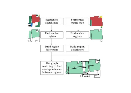
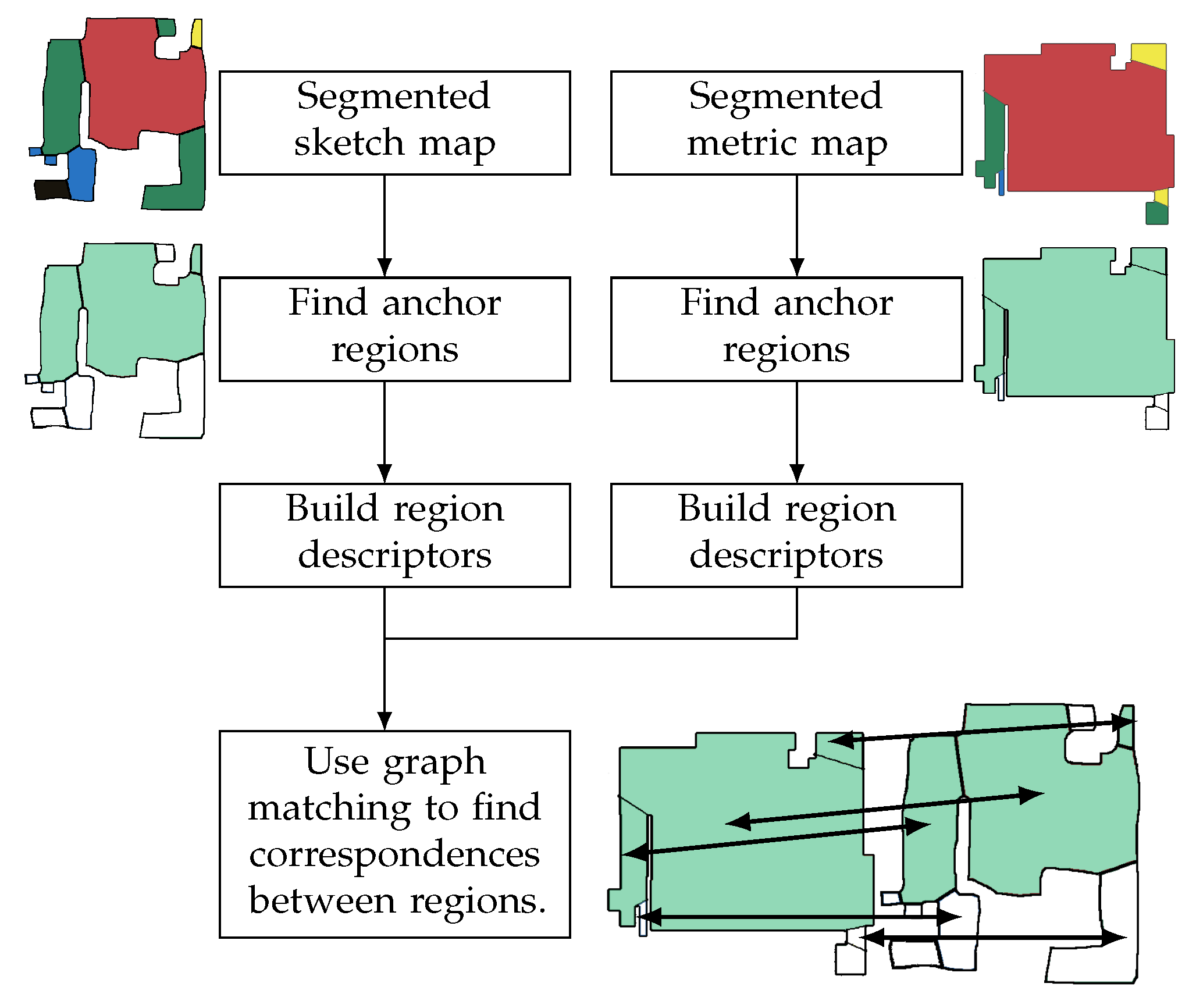
Figure 2.
Flowchart of the Unique Region for Sketch map Interpretation and Matching (URSIM) method. Looking at the example maps, one can see that understanding the sketch map and how it relates to a metric representation of the environment is not straight forward.
Figure 2.
Flowchart of the Unique Region for Sketch map Interpretation and Matching (URSIM) method. Looking at the example maps, one can see that understanding the sketch map and how it relates to a metric representation of the environment is not straight forward.

Figure 3.
Example of a map segmentation on the left and unique regions found using the map attributes on the right. Non-unique regions are left white. (a) MAORIS map segmentation of a sketch map. (b) Coloured are the unique regions found in the map shown in (a) using the size and shape attributes.
Figure 3.
Example of a map segmentation on the left and unique regions found using the map attributes on the right. Non-unique regions are left white. (a) MAORIS map segmentation of a sketch map. (b) Coloured are the unique regions found in the map shown in (a) using the size and shape attributes.

Figure 4.
Examples of correspondences between anchors identified using the Hungarian matching between different map types. Correct correspondences are in grey while incorrect correspondences are in red. While the Hungarian matching algorithm allows determining a reduced set of anchor regions most likely to correspond to each other, one can see that it is often unable to find sufficiently many correct associations between the vertices since the topology of the map is not yet taken into account. (a) shows correspondences between a sketch map and a metric map; the use case of URSIM. While the main room is correctly matched, the smaller regions are incorrectly matched. (b) shows correspondences between two sketch maps. One out of two of the anchor correspondences is correct. (c) shows the correspondences between two sensor maps. Two out of three correspondences are correct.

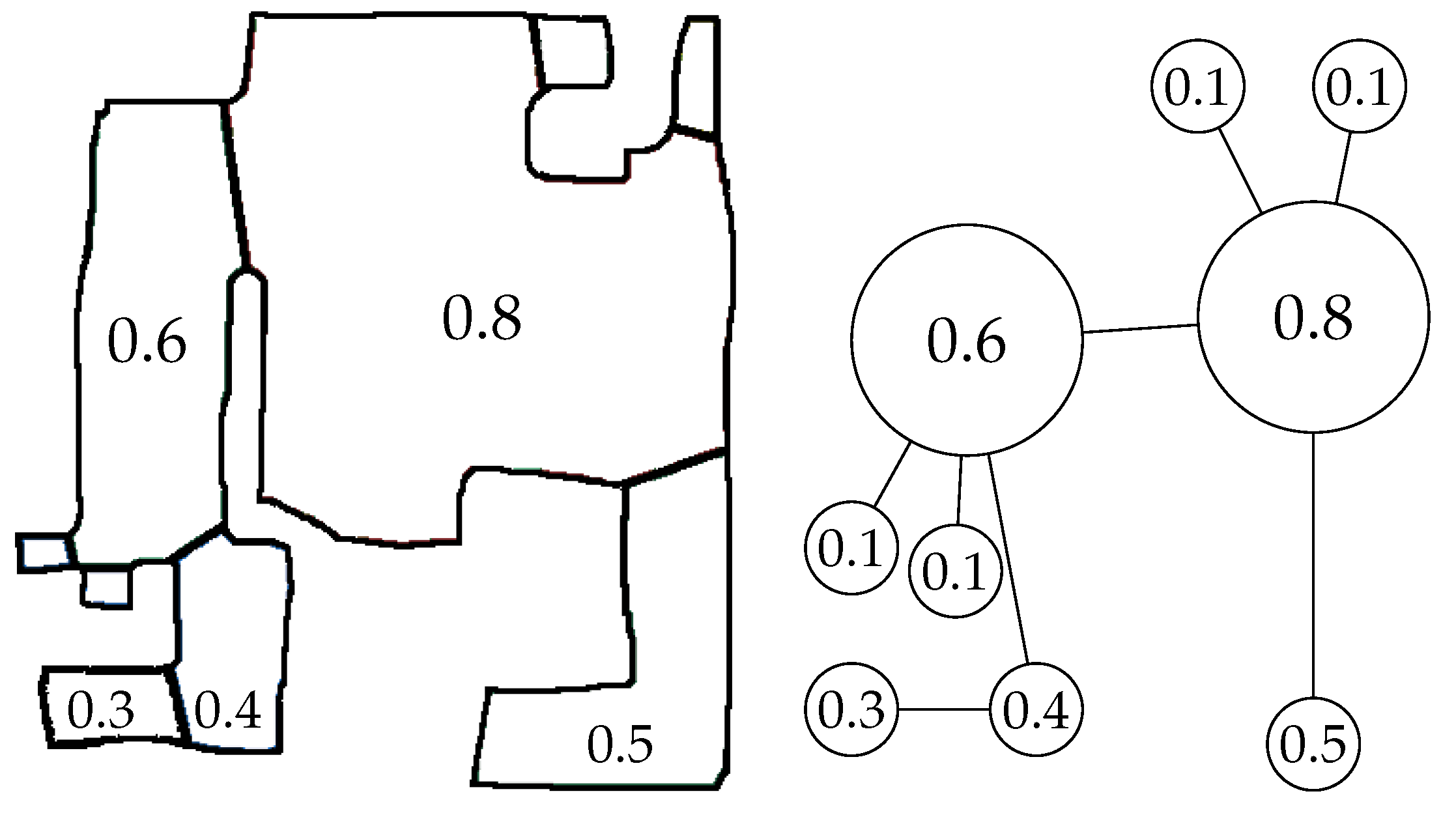
Figure 5.
The sketch map with regions and their corresponding standardized sizes on the left is converted to a graph, with weighted vertices, on the right.
Figure 5.
The sketch map with regions and their corresponding standardized sizes on the left is converted to a graph, with weighted vertices, on the right.

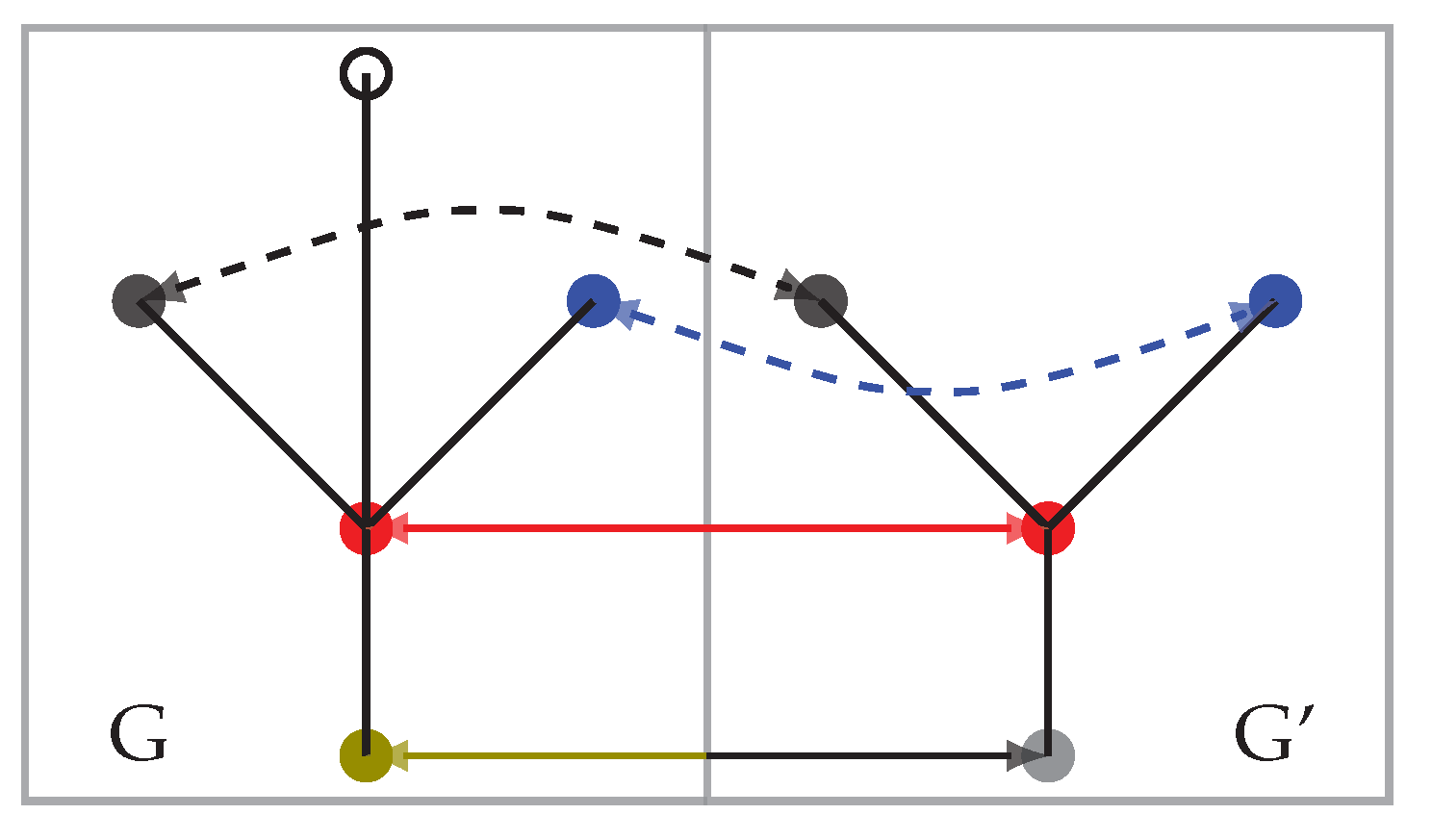
Figure 6.
Illustration of the calculation of the Levenshtein edit distance for correspondences between the neighbors of two vertices in red, where vertex attributes are represented by colors. The blue and black vertices are correctly matched and do not increase the Levenshtein edit distance. On the other hand, the olive and grey vertices are matched but need to change color attribute, thus increasing the Levenshtein distance by one. Finally, the empty vertex on top of the left neighbor needs to be removed, increasing the Levenshtein edit distance by 2: one for the removal of the vertex and one for the removal of the edge. The final edit distance of this matching is 3.

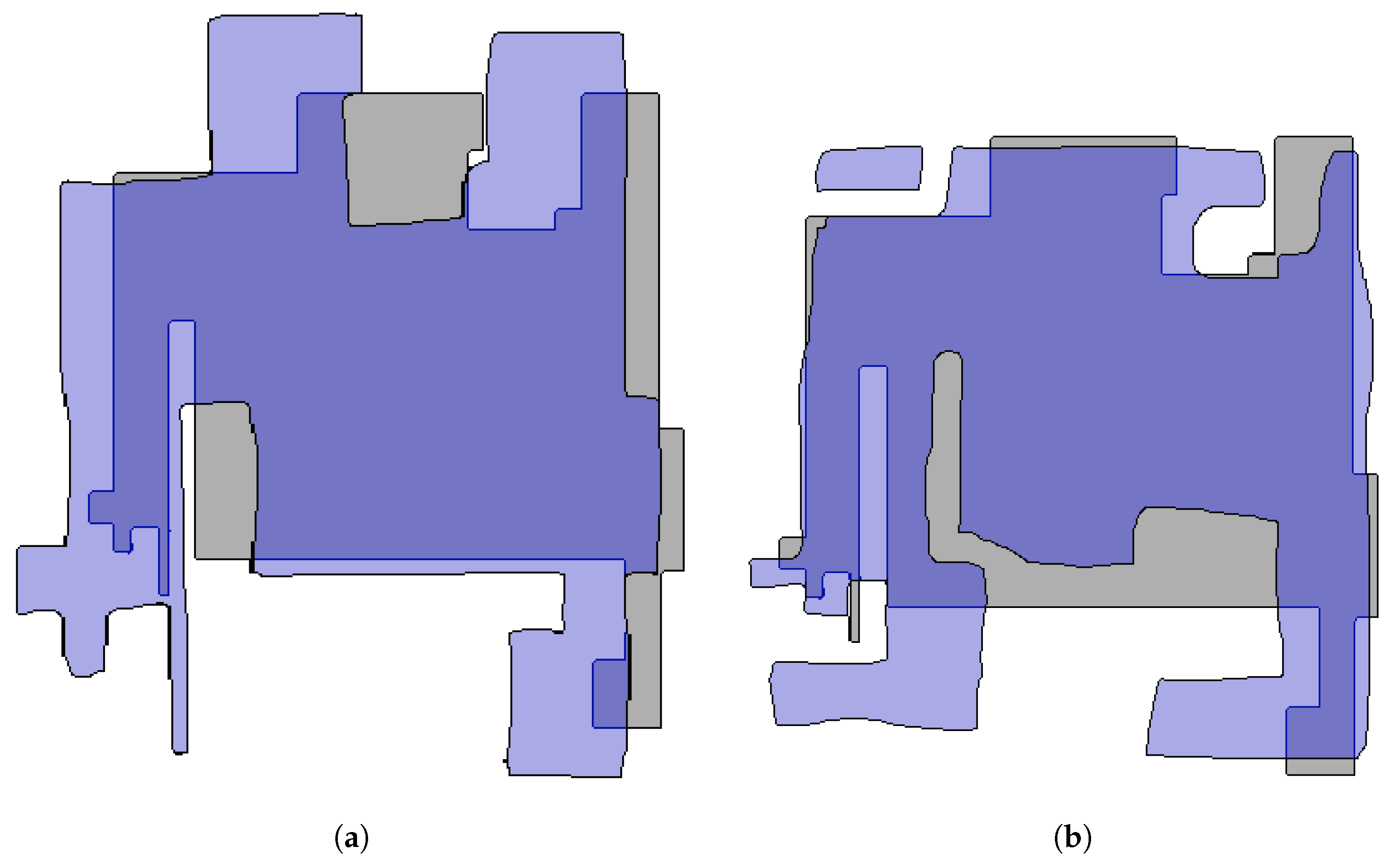
Figure 7.
Regions in one map may have several ground truth correspondences in another map. In this example, one region on the metric map on the left side has ground truth correspondences to three regions in the sketch map. Those three correspondences form a clique.
Figure 7.
Regions in one map may have several ground truth correspondences in another map. In this example, one region on the metric map on the left side has ground truth correspondences to three regions in the sketch map. Those three correspondences form a clique.

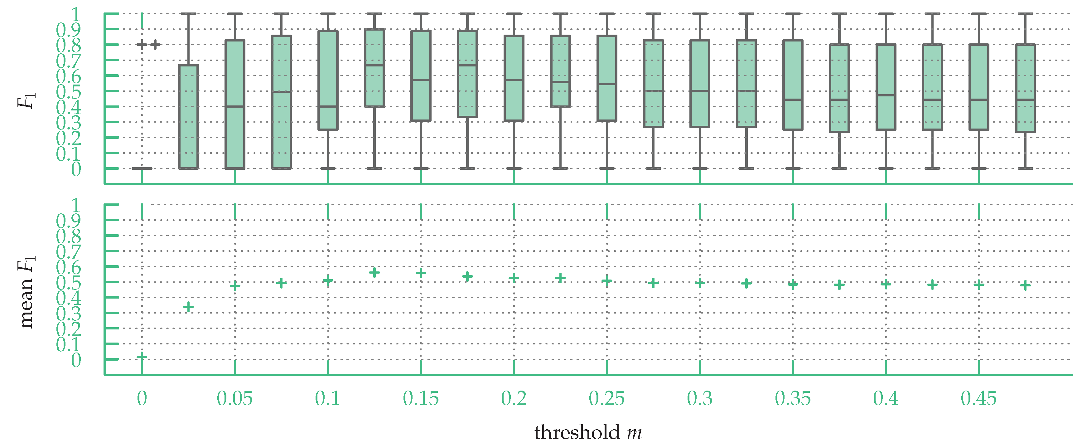
Figure 8.
Mean score using a different number of time samples ranging from 1 to 25 on the sketch map dataset. One can see that the score stays relatively stable and does not depend much on the number of time samples. Using at least 14 time samples leads to slightly better results.
Figure 8.
Mean score using a different number of time samples ranging from 1 to 25 on the sketch map dataset. One can see that the score stays relatively stable and does not depend much on the number of time samples. Using at least 14 time samples leads to slightly better results.

Figure 9.
Flowcharts describing the attributes used to build the descriptors in the tests of Section 6.2. (a) In the first test, , only the topology was used to generate the region descriptors. (b) In the second test, , both the topology and the anchors were used to generate the region descriptors. (c) The third test, , used the topology and the standardized size of regions. (d) The last test, , used the topology, the anchors, and the standardized size of regions.

Figure 10.
Partial sensor maps used by the two users as URSIM’s metric map to build the ground truth correspondences. Both maps represent the same part of the environment. However, since they were built at different times and different doors were opened, the robot mapped a different set of rooms for each map. (a) Partial map used as the metric map for the first user. (b) Partial map used as the metric map for the second user.

Figure 11.
For all maps in the datasets, those charts show for how many maps a given m value lead to the best set of correspondences. On top are the results for the sketch map dataset and at the bottom the results for the partial map dataset. All best-correspondences m values are under for the sketch map dataset and under for the partial map dataset.

Figure 12.
scores when using URSIM with m ranging from 0 to on the sketch dataset. The highest score was found around . However, even better scores could be obtained using different values of m for each sketch map. This shows that m must be carefully chosen on a per map basis.
Figure 12.
scores when using URSIM with m ranging from 0 to on the sketch dataset. The highest score was found around . However, even better scores could be obtained using different values of m for each sketch map. This shows that m must be carefully chosen on a per map basis.

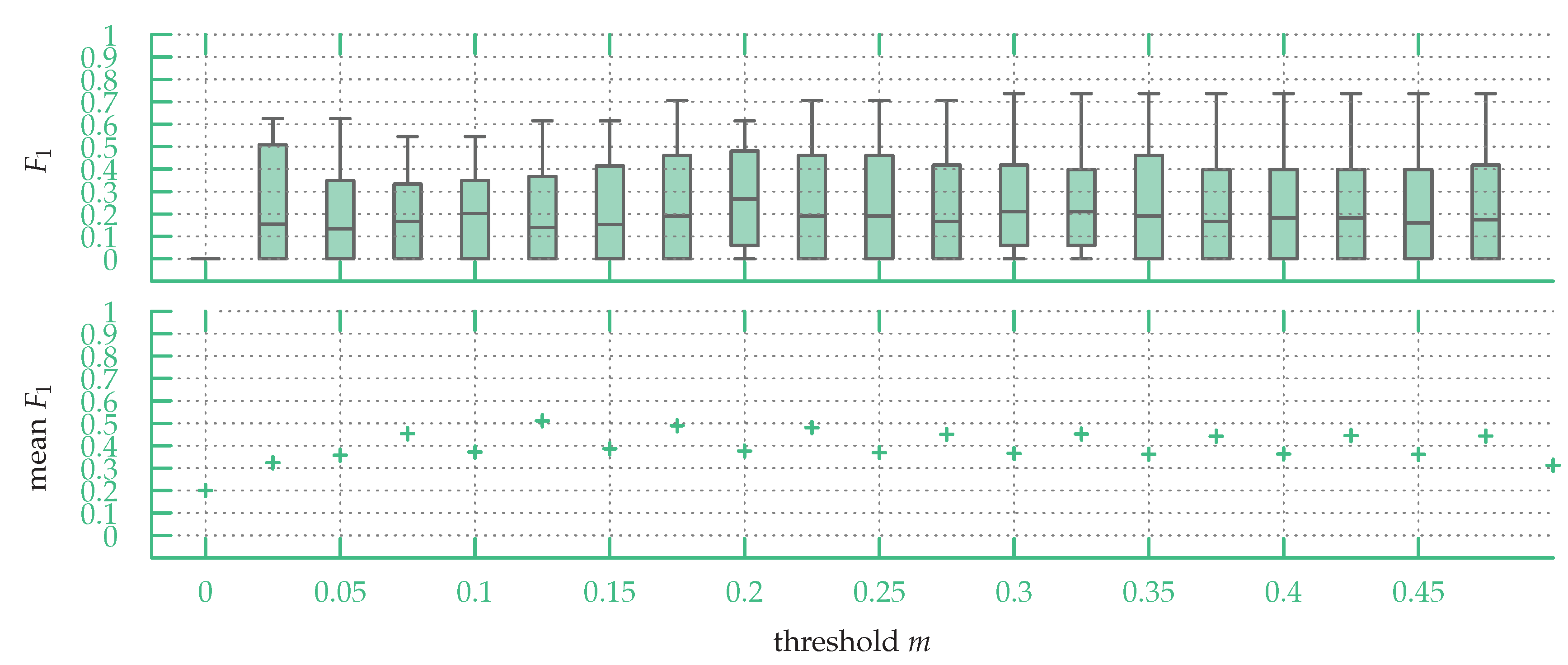
Figure 13.
scores when using URSIM with m ranging from 0 to on the partial map dataset. Above the scores are rather stable but are again not as good as when using different values of m tailored for particular maps. Again, m must be carefully chosen on a per map basis.
Figure 13.
scores when using URSIM with m ranging from 0 to on the partial map dataset. Above the scores are rather stable but are again not as good as when using different values of m tailored for particular maps. Again, m must be carefully chosen on a per map basis.

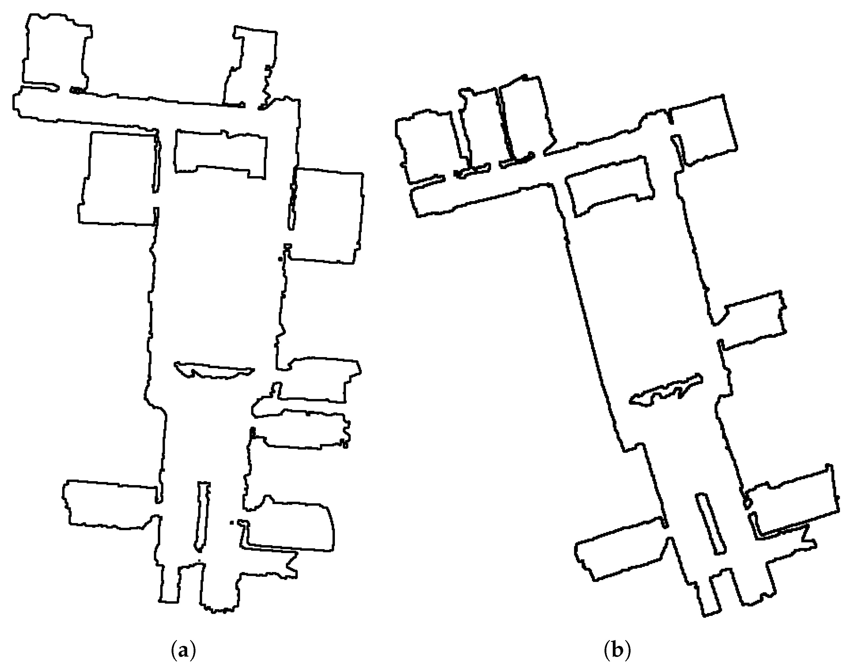
Figure 14.
Sketch map transformed onto the metric map using the affine transformation found by the map matching algorithm of Gholami Shahbandi et al. [17]. The two images correspond to the two best results over the sketch map dataset. One can see that having an affine transformation between the map does not lead to accurate map matching when using sketch maps since local scale errors cannot be taken into account. Hence, the transformed sketch map cannot be used for robot navigation or other tasks. (a) While the maps are correctly centered, the corridors are not matched together due to the differences in local scaling between the maps. (b) Local scale differences make it impossible for the matching algorithm to transform the sketch map onto the metric map.

Figure 15.
Some of the best matches returned by URSIM between sketch and metric maps, and partial sensor maps. Over the three sketch maps in (a–c) only one correspondence is wrong, visible in red in (b), due to the different segmentation between the maps. However, URSIM is not adapted for partial sensor maps and several correspondences are wrong in (d,e). While using methods that rely on metric information leads to incorrect correspondences when using sketch maps (see Section 6.5), adding simple metric information when matching partial sensor maps, e.g., angles between regions or distances, could increase the accuracy of the URSIM’s correspondences for sensor maps.


Table 1.
Median and mean scores over the sketch map dataset. Using the anchors and the standardized sizes as weights on the vertices leads to an increase for both the median and mean score, i.e., increase of the accuracy of the correspondences.
Table 1.
Median and mean scores over the sketch map dataset. Using the anchors and the standardized sizes as weights on the vertices leads to an increase for both the median and mean score, i.e., increase of the accuracy of the correspondences.
| Algorithm | Baseline | ||||
|---|---|---|---|---|---|
| Median values | |||||
| Hungarian | |||||
| VF2 | |||||
| Planar | URSIM: | ||||
| Human VS Human | |||||
| Mean ± one standard deviation | |||||
| Hungarian | |||||
| VF2 | |||||
| Planar | URSIM: | ||||
| Human VS Human | |||||
Table 2.
Median and mean scores over the partial sensor map dataset. The best results are found when using the planar matching with the anchors. When using the anchors to calculate the LFS, the mean stays stable but the median increases. Hence, overall, while more map matches obtained higher scores, maps with a low score are even lower than the maps with a low score when the anchors are not used.
| Algorithm | Baseline | ||||
|---|---|---|---|---|---|
| Median value | |||||
| Hungarian | |||||
| VF2 | |||||
| Planar | URSIM: | ||||
| DAM | |||||
| Mean ± one standard deviation | |||||
| Hungarian | |||||
| VF2 | |||||
| Planar | URSIM: | ||||
| DAM | |||||
© 2019 by the authors. Licensee MDPI, Basel, Switzerland. This article is an open access article distributed under the terms and conditions of the Creative Commons Attribution (CC BY) license (http://creativecommons.org/licenses/by/4.0/).
Share and Cite
MDPI and ACS Style
Mielle, M.; Magnusson, M.; Lilienthal, A.J. URSIM: Unique Regions for Sketch Map Interpretation and Matching. Robotics 2019, 8, 43. https://doi.org/10.3390/robotics8020043
AMA Style
Mielle M, Magnusson M, Lilienthal AJ. URSIM: Unique Regions for Sketch Map Interpretation and Matching. Robotics. 2019; 8(2):43. https://doi.org/10.3390/robotics8020043
Chicago/Turabian StyleMielle, Malcolm, Martin Magnusson, and Achim J. Lilienthal. 2019. "URSIM: Unique Regions for Sketch Map Interpretation and Matching" Robotics 8, no. 2: 43. https://doi.org/10.3390/robotics8020043
Note that from the first issue of 2016, this journal uses article numbers instead of page numbers. See further details here.