Simulation of an Autonomous Mobile Robot for LiDAR-Based In-Field Phenotyping and Navigation

Abstract

The agriculture industry is in need of substantially increasing crop yield to meet growing global demand. Selective breeding programs can accelerate crop improvement but collecting phenotyping data is time- and labor-intensive because of the size of the research fields and the frequency of the work required. Automation could be a promising tool to address this phenotyping bottleneck. This paper presents a Robotic Operating System (ROS)-based mobile field robot that simultaneously navigates through occluded crop rows and performs various phenotyping tasks, such as measuring plant volume and canopy height using a 2D LiDAR in a nodding configuration. The efficacy of the proposed 2D LiDAR configuration for phenotyping is assessed in a high-fidelity simulated agricultural environment in the Gazebo simulator with an ROS-based control framework and compared with standard LiDAR configurations used in agriculture. Using the proposed nodding LiDAR configuration, a strategy for navigation through occluded crop rows is presented. The proposed LiDAR configuration achieved an estimation error of 6.6% and 4% for plot volume and canopy height, respectively, which was comparable to the commonly used LiDAR configurations. The hybrid strategy with GPS waypoint following and LiDAR-based navigation was used to navigate the robot through an agricultural crop field successfully with an root mean squared error of 0.0778 m which was 0.2% of the total traveled distance. The presented robot simulation framework in ROS and optimized LiDAR configuration helped to expedite the development of the agricultural robots, which ultimately will aid in overcoming the phenotyping bottleneck.

1. Introduction

Climate change, population growth, and labor shortages pose immediate threats to the sustainability of global agriculture [1]. To ensure global food and fiber security, crop yield must increase and be made more robust to keep up with climate change. This can be achieved through breeding programs, which selectively cultivate crop genotypes with favorable phenotypic traits, such as higher yield and stress tolerance [2]. Crop phenotyping is done primarily by hand and, thus, does not allow for efficient, large-scale selective breeding [3]. In-field, high-throughput phenotyping (HTP) technologies are being developed to address this challenge, but repeatedly gathering phenotypic data on a large scale still presents a considerable bottleneck [4]. To address this phenotyping bottleneck, autonomous robots equipped with advanced sensor payloads have been developed in recent years to gather phenotypic data consistently and with a high throughput. Autonomous robots are particularly useful in phenotyping applications since they reduce the human labor needed to gather large amounts of data about crops. Robots can work continuously for long periods of time and at lower cost than humans, thereby allowing for a higher throughput of data collection.

Light detecting and ranging (LiDAR) sensors are one of the most widely used sensor systems in robotic platforms because of their ability to give accurate distance measurements without contact. LiDAR is increasingly being used in the field to generate 3D point clouds of crops for phenotypic analysis [5] as well as low-cost crop navigation [6]. A 2D LiDAR can generate point cloud data to determine important phenotypic traits of cotton plants, such as canopy height and plant volume [7]. Various methodologies have been used to calculate canopy volume from LiDAR Data. One study used a trapezoidal based algorithm where the profile of the LiDAR point cloud was used to calculate volume [8]. Another study calculated volume by voxelizing a point cloud and then extracting the volume [9]. Previous studies showed that plant height and volume are important parameters for geometric characterization and are highly correlated with final crop yield [10,11,12].

A static 2D LiDAR measures distances between objects on an xy plane. These 2D scans can be combined to create a 3D point cloud by moving the 2D LiDAR and applying the transformation of the sensor’s movement to the 2D scans in an inertial frame. The advantage of actuating a 2D LiDAR is that it can be used to generate a 3D point cloud at a lower cost than that of a typical 3D LiDAR sensor [5]. Most in-field applications of 2D LiDAR for high throughput phenotyping involve statically mounting the 2D LiDAR on a mobile platform and moving it directly overhead or to the side of the ground plant [5,7,13,14,15]. Agricultural mobile robot with side-mounted LiDAR units have been used to monitor health of status of crops [16,17]. Two recent studies on cotton plant phenotyping using 2D LiDAR have used systems with a 2D LiDAR in an overhead configuration in which the 2D LiDAR is perpendicular to the ground plane [7,18]. It is important that additional 2D LiDAR configurations are evaluated to determine their efficacy in measuring plant phenotypic traits. On a mobile robot, however, the most common strategy for using 2D LiDAR is in a “pushbroom” configuration. With this configuration, the LiDAR sensor is angled obliquely to the plant, and when the mobile base moves, the LiDAR scan is “pushed” and a 3D point cloud is generated. This pushbroom configuration has been used by mobile robots to navigate between crop rows [19,20]. Another class of 2D LiDAR configuration for 3D point cloud generation involves actuating the LiDAR sensor while it is mounted on a mobile base; this allows the 2D LiDAR to capture additional angles for distance measurement. 2D LiDAR has also been configured with a “nodding” configuration, such that the LiDAR is on a servo and “nods” back and forth to generate a 3D point cloud [21]. In a similar but slightly different configuration, Zebeedee is spring-mounted 2D LiDAR that has been used extensively for 3D mapping commercially [22].

Navigation of an autonomous robot is a challenge especially in agricultural fields where the environment is semi-unstructured with uneven ground surfaces, changes daily with dust and fog affecting sensor observations, and lacks of unique localization features [23]. Efficient navigation strategies are critical to an autonomous agricultural robot in the field due to battery constraints which limit operation time. Additionally the navigation strategy must output valid velocities that are within the kinematic constraints of the robot. GPS and range sensor-based navigation strategies are most commonly used methods.

A global positioning system with real time kinematic (RTK) differential correction can provide highly accurate global positioning to a centimeter level when it has an unblocked view of the satellites from the Global Navigation Satellite System (GNSS). Field robots have been developed by researchers to utilize GPS guided navigation for waypoint navigation in a world frame without any active obstacle avoidance [24,25,26,27,28]. These waypoints are chosen to allow the rover to follow a path based on the assumption that no additional obstacles will be introduced to the rover’s path. For example, “pure pursuit” is a popular path tracking algorithm that has been used extensively for autonomous navigation due to its simplicity and computational efficiency [29,30]. This navigation algorithm is a geometric method which outputs an angular/linear velocity that will move the robot in an arc to get to the desired robot position. An additional advantage of the pure pursuit algorithm is its output of a smooth path that is feasible for a differential drive robot and easily tunable with parameters such as look ahead distance. Robotanist is an agricultural robot that uses RTK GPS and “pure pursuit” as its navigation algorithm to go from point to point [19]. PID control has also been used as a path tracking navigation system due to its robustness and simplicity in implementation [31,32]. The disadvantages of GPS-based navigation strategies include that field robots may fail if the environment changes significantly or anything blocks the path of the rover [33]. Additionally RTK GPS is prone to inconsistent localization due to occlusion, attenuation and multipath errors and thus it requires redundancy and continuous fail-safe checking [34]. Another disadvantage for RTK GPS is that it is costly and is cost-prohibitive in multiple-robot implementations [35].

For inter-crop row navigation, GPS navigation is sometimes insufficient for the small heading and position corrections that are needed to successfully move between crop rows. In these cases, sensors such as cameras and range sensors (e.g., LiDAR and ultrasonic sensors) have been used extensively to perform local crop row navigation which involves determining the relative positioning (heading and distance) of the robot between crop rows [24]. The main goal of this localization strategy is to maintain proper distance from the left and right crop rows to avoid collision [36,37,38]. In one study, probabilistic techniques such as a Kalman Filter and Particle Filter were used alongside a 2D LiDAR for localization in-between crop rows to perform appropriate control actions [39]. One significant hurdle using 2D LiDAR for navigation is the occlusion resulting from plant leaves and branches, which can negatively affect the characterization of the crop rows and cause navigation to fail [37]. Another important drawback of the range sensor-based navigation strategy is that it does not localize a robot in a global frame for complete autonomous control.

Development of robotic platforms is time/cost intensive and complex, and, therefore, simulation is being used increasingly to test and validate robotic platforms as well as their sensors for their ability to perform agriculture sensing as well as navigation [40,41]. Simulation allows for low-cost and quick robotics testing and validation, which results in a large initial focus on broad strategies. In agricultural robotic simulations, the testing environment can be recreated to match specific agricultural use cases and robotic sensor platforms, and algorithms can be tested for efficacy and efficiency [36,42,43]. Full control strategies can be tested and developed with simulated sensors completing a feedback loop. Many agricultural robot drive systems and navigation techniques have been developed and tested in simulation prior to successful implementation [44,45,46]. A variety of simulation tools, such as V-REP, Gazebo, ArGOS and Webots, have been used and compared for robotics simulation in agriculture [40].

This paper proposes a simulated mobile robot configuration that can collect phenotypic and crop row data and autonomously navigate between crop rows using GPS waypoints and 2D LiDAR. Using a “nodding” LiDAR configuration [21], 3D point cloud data were generated and used for phenotyping as well as for navigation between crop rows. This actuated LiDAR configuration was tested in a high-fidelity simulation environment that simulated a cotton field with the occluding effects of cotton plants as well as the slippery, uneven terrain of a crop field that may affect LiDAR-based inferences and navigation.

2. Materials and Methods

2.1. ROS Mobile System Overview

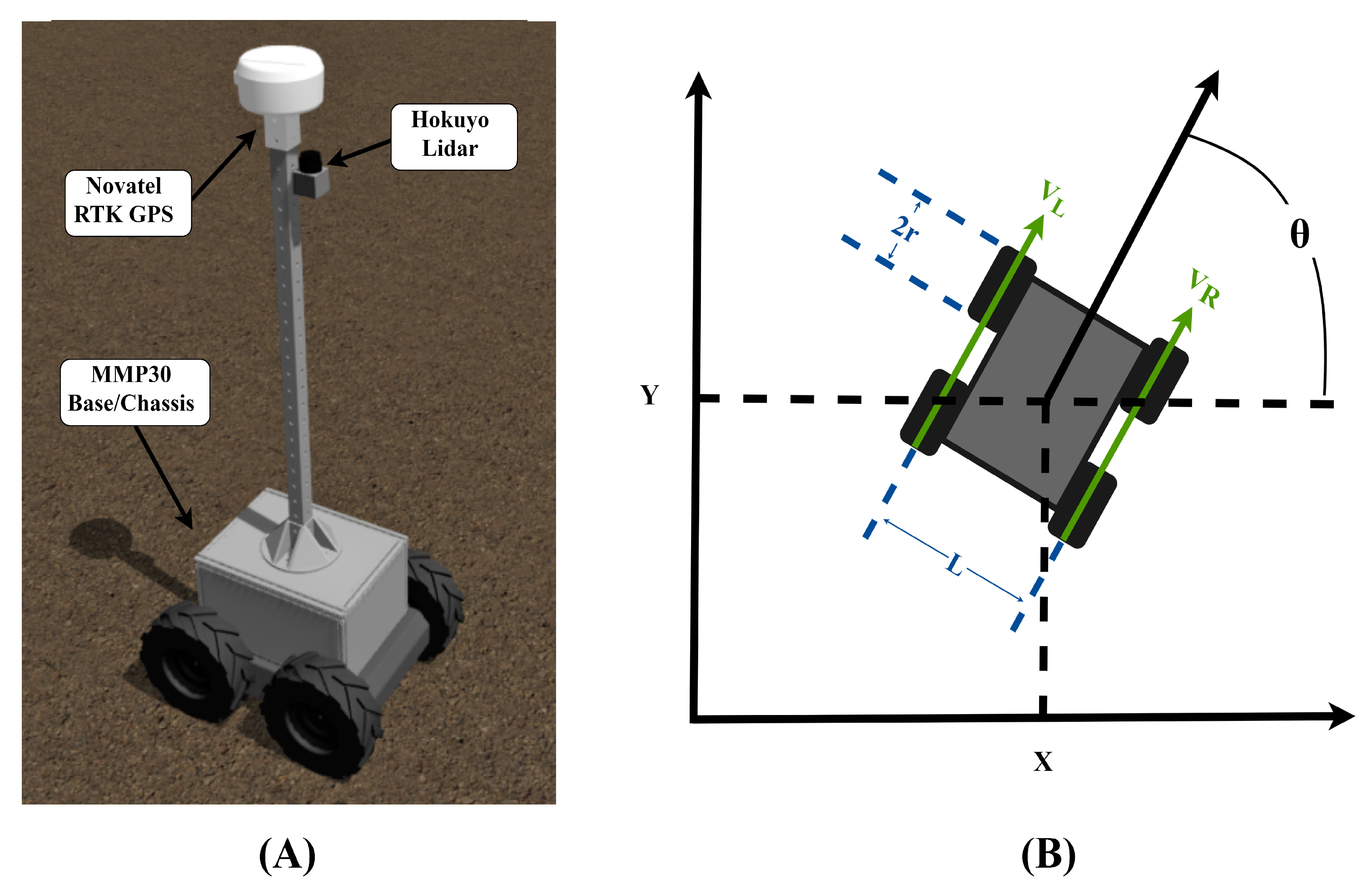
The system modeled in this paper is an unmanned ground vehicle (UGV) called the Phenotron. The Phenotron is a 4-wheel rover that utilizes a skid steer drive system. The sensors on board the Phenotron include a Hokuyo UTM-30LX 2D LiDAR, VectorNav Inertial Measurement Unit (IMU), and a Novatel RTK Global Positioning System. A CAD model for the drive system was based on a commercially available MMP30 model (The Machine Lab, Fort Collins, CO, USA).

The Robot Operating System (ROS), an open source meta operating system, was used for the development of the Phenotron. ROS provides a standardized communication platform and system for code reuse for applications like autonomous navigation and mapping. Gazebo, an open source physics simulator, was used to simulate the cotton fields and the Phenotron. Gazebo was chosen for use in this simulation study because of its better integration with ROS and its completely open-source nature, which allows for a more extensible and widely-usable simulation. ROS was also used as the underlying communication network between the simulated sensors, the environment, and the ROS packages and open source code used for robotics development.

To import the 3D model into the Gazebo simulator, a universal robot description format (URDF) file was created where its structural and locomotion elements were defined. The SolidWorks CAD model was exported into a URDF file using the solidworks_to_URDF_exporter add-in within SolidWorks. The exporter allows the user to export a CAD assembly and its kinematic tree to a properly linked URDF file alongside its corresponding CAD files (Figure 1). Within the URDF, every part of the robot is defined by links and joints, with each link and joint defining various properties of the robot. The wheels are defined as links that contact the ground as the locomotion elements of the rover and have a “continuous” joint that allows for continuous rotation about one axis relative to the chassis. This continuous joint is linked from the ROS to the Gazebo simulator by defining a transmission tag that specifies a velocity joint hardware interface, which enables each wheel to send velocity commands.

The differential drive motion of the Phenotron was controlled using the open source ROS package diff_drive_controller. The diff_drive_controller package was configured by referencing the transmission/joints defined in the URDF file and the dimensions of the rover. The diff_drive_controller accepts a geometry/twist message type that defines the linear and angular velocities along the XYZ axis. The right and left wheel velocities (Figure 1) required to meet the commanded goal velocity for the rover were computed and the velocity commands were sent to the rover. The diff_drive_controller package also computes the odometry of the Phenotron-simulated rover based on the velocities of the right and left wheels. Based on the odometry equations of a standard differential drive system (Equations (1)–(3)), $\dot{\theta }$ describes the angular velocity of the rover based on the linear velocities of the right and left wheels $V_R,V_L$ in addition to the distance between the right and left wheels of the rover (L). $\upsilon$ is the linear velocity of the rover. With the linear and angular velocities and the heading $\theta$ of the robot, the linear velocities $\dot{x}$ and $\dot{y}$ in the world frame can be found.

$$\dot{\theta }=\frac{V_R-V_L}{L}$$

(1)

$$\upsilon =\frac{V_R+V_L}{2}$$

(2)

$$\left[\begin{array}{c}\dot{x}\\ \dot{y}\\ \dot{\theta }\end{array}\right]=\left[\begin{array}{cc}cos\theta & 0\\ sin\theta & 0\\ 0& 1\end{array}\right]\left[\begin{array}{c}\upsilon \\ \dot{\theta }\end{array}\right]$$

(3)

Localization sensors on the Phenotron were simulated in Gazebo through open source plugins that create a sensor interface between the simulator and the ROS. Sensor simulator Gazebo plugins for the Global Positioning System and Inertial Measurement Unit were sourced from the hector_gazebo_plugin by Team HECToR (Heterogenous Cooperating Team of Robotics) of Technische Universitat Darmstadt [47]. The desired sensors/plugins are referenced in the URDF file. The sensor data were published automatically in the ROS topics list and are available for further use. For the 2D LiDAR scanner, a Hokuyo LiDAR was used with the Gazebo plugin “gazebo_ros_head_hokuyo_controller”. To match real specifications of the Hokuyo LiDAR, noise was included in a parameter for the plugin such that the noise followed a Gaussian distribution with a standard deviation of 0.01 m. Thus, 99.7% of samples are within 0.03 m of the true reading, which achieves a +/− 30 mm accuracy at ranges less than 10 m [48]. The simulated LiDAR has an update rate of 40 Hz. For GPS simulation, a real time kinematic (RTK) GPS was simulated including additive Gaussian noise with a standard deviation of 2 cm. With this noise factor, 70% of the time the accuracy of the GPS measurements were within 2 cm, thereby mimicking the accuracy of an RTK GPS that can achieve up to a 1 cm level positioning accuracy. The simulated GPS and IMU had an update frequency of 40 Hz. The "robot_localization" package is used to output a state estimate by using an extended Kalman filter and fusing the simulated RTK GPS with the inertial measurement unit and wheel encoder odometry. The robot localization package has an update rate of 30 Hz. For the simulated Hokuyo LiDAR, the scan frequency was 40 Hz.

2.2. Simulation World

A high-fidelity cotton plant model was designed within Sketchup^TM and imported into Gazebo as a 3D graphic file. Once a model of a single plant was created, the plants were then rotated randomly and grouped together within Sketchup^TM to create plots. The plant heights are modeled to be 1.2 m in height and 1.15 m in width and length (Figure 2). The plots themselves were made to be 3 m in length. The plot rows were spaced 1 m apart to mimic an experimental cotton field. The size and spacing of the plots were based on a study where multiple cotton plant cultivars were analyzed in terms of growth [8]. There were five plants within each plot with a 0.6-m distance from each other to have around 50% overlap to simulate plant occlusion and density.

The ground was constructed in Sketchup^TM using the sandbox tool. Bumps were simulated by creating pyramid-shaped protrusions in the plane’s mesh with the height of the bumps being 2 cm. This height was decided based on a reference [49] in which agricultural terrain was classified. Four 1 × 1 m squares with arbitrarily chosen “bumps” were put together randomly to make a 2 × 2 m (Figure 2). In this configuration, there was a 100% chance that the rover would encounter some type of bump disruption per two meters of travel. Then these 2 × 2 squares were multiplied to create a 60 m by 60 m field. A testing field of 4 rows was created in which each row consisted of 3 plots and in which each row was spaced 1 m from each other (Figure 3).

2.3. Experiment/Analysis Phenotypic Analysis

LiDAR Configurations

Multiple LiDAR configurations that have been used in HTP were configured and tested on a simulated cotton field. Their ability to correctly identify the height and volume of the plants using a 2D LiDAR was evaluated. The proposed actuated LiDAR configuration, also known as “nodding,” was tested against 3 common static LiDAR configurations used in agricultural robots for phenotyping: Tilted, Side and Overhead. The Tilted configuration was angled 45 degrees down from horizontal, aimed obliquely at crops at a height of 1.5 m (Figure 4A). The Side configuration was angled perpendicular to the ground, facing directly to the side of the crops at a height of 0.75 m (Figure 4B). And finally, the Overhead configuration was pointed towards the ground and facing the crops directly overhead (Figure 4C). The proposed LiDAR configuration actuates the 2D LiDAR in a nodding motion, similar to the Tilted configuration. However, the LiDAR angle is relative to horizontal changes over time (Figure 4D). This strategy is proposed to address leaf occlusion because some features are lost as the LiDAR needs a clear path to detect the profile of the plant canopy accurately, and, as such, multiple angles of detection would assist in this characterization [6]. For the nodding configuration, the LiDAR is rotated while the mobile base is static and the angled LiDAR scans from 0 radians (parallel to the ground) to 0.4 radians (22.9 degrees) towards the ground. The LiDAR is actuated at a step increment of 0.005 radians (0.286 degree) at 10 Hz which results in a rotational velocity of 0.05 radians a second (2.86 degrees) and a complete nod cycle time of 8 s.

Since only a 2D LiDAR was used, each scan of the LiDAR needed to be stitched together to generate a 3D point cloud for analysis. The laser assembler ROS package was used to initiate a server service that could be called upon to begin assembling scans together at specific time intervals. The frame in which these laser scans were assembled was set with the laser assemble ROS package and in the global “map” frame (Figure 5). This transform frame is generated by the "robot_localization" package. The “laser_assembler” service call responds with a point cloud that is then published to an ROS topic. This assembled laser point cloud is then downloaded as a PCD file using the pcl_ros package, which listens to a topic and then saves it to a directory.

The ability of the LiDAR configurations to obtain the two main phenotypic traits of cotton plants, height and volume, was tested (Figure 6). For each of the 4 LiDAR configurations, the simulated autonomous robot was given a velocity command to go forward and continuously collect LiDAR data for a single row containing 3 plots (Figure 5). Each configuration collected point cloud data (PCD) from a single side of the plot for phenotyping estimation. After data collection, the resulting PCD was post processed in MATLAB. A region of interest (ROI) was manually selected for each plot for processing, then the ground floor was determined by using the random sampling consensus algorithm (RANSAC). Once determined, the ground floor was also removed, although the height of the ground plane was recorded as the baseline for height prediction.

To obtain plant height, the LiDAR data were projected on the XZ plane such that height measurements were calculated along the axis that the mobile rover base traveled. Then, peaks were filtered from the height data such that each peak was higher than the peaks around it at a certain distance threshold [10].

To obtain the ground truth for plant volume, the CAD model for the cotton plot was voxelized with cubic centimeter voxels which are cubic volumetric shapes representing regularly sampled spaces that are non-homogeneously filled. The voxelization of a CAD model allows for the computation of volume taken up by the CAD model with a predetermined sized cubic shape. The voxelized plant model was put into a CAD program called Blender where the 3D print tool was used to determine the volume of a single voxelized cotton plot. The volume of a single plot was experimentally determined from the point cloud data using the MATLAB boundary function with its default shrink factor of 0.5. Shrink factor is a scalar value ranging from 0 to 1 where 0 results in the convex hull of the points while 1 corresponds to the tightest single-region boundary around the points. As such when the shrink factor was 1, due to making the tightest boundary around the point cloud, the volume estimate is much lower than when the shrink factor was 0 where only the outer most points are used for the generated hull. The default value for shrink factor of 0.5 was kept as it was a neutral parameter for volume estimation.

2.4. Experiment/Analysis Nodding LiDAR Configuration for Navigation Through Cotton Crops

As the rover moved through the crop row, the 2D LiDAR was actuated in a certain “nod” window. In this nod window, 2D laser scans were stitched together to generate a 3D point cloud at a certain look ahead distance. Since the rover is in the middle of the two rows, the field of view of the 2D LiDAR is large enough to capture both the left and right crop row simultaneously at each nod. While the LiDAR unit is actuating, the laser assembler node is continuously listening to the LiDAR topic and the transform of the LiDAR unit to assemble the individual scans and generate a point cloud every 8 s which is the time needed to complete a single nod. The Hokuyo LiDAR is continuously being actuated to make sure that the crop rows are being characterized even while moving. The LiDAR scans are still being transformed and assembled relative to the movement of the rover itself as it is moving by using the state estimate and transform provided by the "robot_localization" package. The output of the "robot_localization" state estimation is at the same frequency as the simulated Hokuyo LiDAR, as such the pose of the robot is accurately considered even while moving. At the end of each “nod” action, the generated point cloud was sent to a Python service node in the sensor_msgs/PointCloud2 message format. This Python service, which is detailed later, returned the angles of the left and right crop row as well as their distance away from the rover. Based on this service response, the navigation module performs a control action which would include angular and linear velocity for 0.25 s. Then the rover waits for the next control update as the nodding LiDAR gets actuated and the point cloud data gets processed. The main goal of the LiDAR based navigation strategy was to stay parallel and equidistant with the left and right crop rows. Each point cloud generated for every iteration of the looped navigation control were combined based on the distance traveled by the rover as calculated by the "robot_localization" package.

LiDAR Processing Strategy

Using the same laser assembler package discussed above, the nodding LiDAR scans were assembled within a specific tilt window. The tilt window was defined as the angle range at which the nodding actuation occurs and the corresponding 2D laser scans assembled into the point cloud. A row_characterization service server was created that accepts a point cloud from the assembled point cloud topic. The row_characterization server utilizes the open 3D point cloud library, a library for point cloud data processing. The point cloud data were downsampled and voxelized and then split into the left and right rows (Figure 7). Each of these rows were then filtered using a radius outlier filter and then a RANSAC algorithm was used to fit a line through the left and right rows. The row_characterization server returned the average angle of the left and right crop rows as well as the distance of left and right rows from the robot itself.

2.5. ROS Node Structure

A complete ROS topic and node structure was developed to mimic the topic and information structure of the real rover (Figure 8). The data from the inertial measurement unit, wheel odometry, and GPS topics were combined using an extended Kalman filter using the robot localization package to get an accurate pose estimate. The robot localization package also handled creating the various transforms needed to convert GPS waypoints into goals in the rover’s frame. The GPS topic was converted to UTM coordinates by the gps_common package for Euclidean-based navigation. A navigation module was developed to handle all control actions of the rover and the implementation of the algorithm described above. An ROS service was created that takes a point cloud input in the sensor_msgs/PointCloud2 ROS message format. The service call processed the point cloud and characterized the crop row point cloud to give the angles of the left and right crop rows and the distance between them. The navigation module then processes the crop row information and performs the appropriate control action. ROS-control and Gazebo are simulation-based processes that implement commands to actuators and simulate all sensor and physical interactions with the rover.

2.5.1. Control Loop for Crop Row Navigation

A feedback system with two error signals was created to correct the rover to ensure it is traveling safely between the crop rows. One error signal includes an angle of the rover relative to the left and right crop rows. Ideally, the robot should be completely parallel to the left and right rows. If the crop rows are angled from the rover’s perspective, the angles of the left and right crop rows are averaged and then this is output as an error for row heading. The average of the left and right rows was used as the error signal. The second error signal was the difference in distance between the robot and the right and left rows. Ideally, the difference between the two rows would be zero, which would mean that the right and left rows are equidistant from the robot, which is the desired position of the robot. If the position was closer to the right row than the left row, this would be output as an error. For the heading error and the distance error there were threshold values for registering errors to make sure that the control action was not enacted for trivial error values in heading and distance. The error values for heading and distance are multiplied by corresponding weights C1 and C2 to control the amount of impact each error signal has on the control action (Figure 9). Then both error signals are summed and input into the PID controller. The PID controller was tuned through trail and error to output the appropriate angular velocity for 0.25 s to correct the heading and the centering of the rover relative to the crop rows. For each control step, there was always a linear velocity in the x-axis frame to ensure the robot keeps on moving forward. The control loop iterated based on the subsequent error signals generated by the actuated LiDAR until the stop condition is met as described by the complete navigation algorithm detailed below.

2.5.2. Complete Navigation Algorithm

A simple navigation algorithm was implemented for use with the LiDAR based navigation strategy (Algorithm 1). The LiDAR based navigation strategy was designed to be able to move within crop rows despite occlusion and misaligned crop rows without any global positioning. However, for use in a crop field with multiple rows, additional intelligence is needed. An algorithm is proposed that switches between the LiDAR based navigation, which is robust in navigation between crop rows, and a GPS-based navigation strategy, which ensures that the robot is going to the correct user-defined crop row. The GPS guided navigation algorithm used is called the Pure Pursuit, which finds the linear and angular velocity needed to go to a specific point in space [19].

Algorithm 1: Complete Navigation Algorithm

The proposed algorithm creates a robust navigation strategy that is extensible and re-configurable for different navigation plans for the rover. The main parameter in this algorithm is the distance between crop rows ($d_{cr}$ ) (Figure 10). Initially, the rover starts using the LiDAR-based navigation strategy when it goes straight while facing the next GPS waypoint. However, when the rover is within ($d_{cr}$) distance of a GPS waypoint, it switches to the Pure Pursuit algorithm. The Pure Pursuit algorithm guides the rover to the waypoint (A GPS coordinate as well as heading), which faces the next waypoint on the list of waypoints given by the user (these are points between one crop row plot and the next to define the path the rover will take). When the rover gets to the waypoint at a sufficient tolerance and faces the next waypoint, the navigation algorithm now switches back to the LiDAR-based navigation strategy. The rover goes straight while performing an appropriate control action to stay centered between crop rows until it gets within $d_{cr}$ of the next waypoint and the algorithm repeats until the last waypoint. In the case where it reaches the end of the crop row and must go to the next crop row, it checks the ($d_{cr}$) parameter and automatically switches to Pure Pursuit to get into position to implement the nodding LiDAR-based navigation. This process will continue until the last waypoint is reached. With the switching dual strategy, fewer waypoints are needed to be given to the rover, and by being given only the waypoints at the end of each row, the LiDAR-based navigation strategy can maintain distance between crop rows successfully.

The navigation strategy was tested in a simulated crop field under two scenarios. In the first scenario, the crop rows were parallel with each other and waypoints were provided for each plot totalling 12 waypoints. In the second and more challenging scenario, the crop rows were not parallel, which allowed for the testing of the robustness of the navigation strategy to make corrections for non-parallel crop rows. Additionally, the test waypoints were given only at the end of the crop rows totalling 6 waypoints, so the LiDAR-based navigation strategy had to navigate through the entire crop row by itself. The ideal path was determined as being equidistant and parallel to the crop rows.

3. Results and Discussion

3.1. Phenotyping and Navigation Results

The nodding, tilt and side configurations had comparable volume results with an average percent error of 6%. Of the 3 configurations, the nodding configuration had the highest volume error of 6.6% ± 4.8%. The tilt and side LiDAR configurations had average errors of 5.7% ± 3.4% and 6.6% ± 2.8%, respectively (Figure 11). The tilt and nodding configurations had the most similar results, however the nodding configuration performed slightly worse due to the LiDAR actuating while moving over the uneven ground. The side configuration performed slightly better than the tilt and nodding configurations due to having the best side profile of the plot as well as being the best suited for the convex hull method of volume estimation. The side configuration was able to get the ends of the plots which due to getting a hull wrapped around it, compensated for not having a view of the width of the plot. The overhead configuration had the highest average percent error for volume at 15.2% ± 5.7%. While all the volume estimations were underestimates compared to the ground truth, the overhead volume estimate was much lower. This underestimation from the overhead configuration was due to the LiDAR only being able to view the canopy of the plot and missing the side profile for volume estimation.

For plant height prediction, all configurations were able to perform within a low percentage error with an average percentage error of 2.7%. The overhead configuration performed the best with a 1.3% ± 0.87% average error. This is because a direct overhead angle that obtains a perpendicular-to-the-ground cross section collects more z-axis data from the plot. With this overhead view angle, the LiDAR was better able to characterize the height of the plant relative to the ground because each scan captured the entire top of the crop of interest as well as the ground to the side of the plot. The overhead configuration is more robust in calculating errors for height estimation compared to the tilt (4.2% ± 0.69%) and nodding (4% ± 0.14% which are pointed downward obliquely into the crops and does not have a unobstructed view of the ground. In the presence of external error factors such as an uneven ground, the overhead configuration is better able to compensate for height disturbances by more effectively mapping of the ground which was used as the height baseline by the RANSAC algorithm. Height detection using configurations such as side (2.8% is sensitive to bumps and noises, as they have a more limited angle on the z axis cross sections onto the plots. For height estimation all the LiDAR configurations underestimated the height of the cotton plant because the height estimation was an average of the top profile of the attained point cloud data. Additionally the uneven ground has only protruding bumps which elevated the rover and LiDAR, making plant measurements smaller.

Overall this phenotyping study determined that the proposed nodding LiDAR configuration achieves comparable accuracy in volume and height estimation when compared to commonly used configurations such as side and tilt. The nodding configuration performed height and volume analysis with relatively low error, similar to that of tilt and side. The overhead configuration heavily underestimated volume although it performed height analysis with the lowest error. The main advantage of using the proposed nodding configuration is that while it can be used to phenotype and perform competitively with other commonly used LiDAR configurations, it can also be used for navigation while the other configurations cannot.

Results showed that the navigation strategy performs well in both testing scenarios. In the first scenario where all crop rows were parallel and waypoints were given between each crop plot (As shown by the red circles) (Figure 12A) the root mean squared error was 0.0225 m with 32.5 m of travel across three rows, indicating the navigation strategy performed with 0.06% drift from the ideal path. (A video of this first navigation test is provided in the Supplementary Materials). In the second and more challenging scenario, the LiDAR based control algorithm would have to navigate correctly from one plot to the next (Figure 12B). In this scenario the root mean squared error was 0.0778 m with 38.8 m of travel resulting in 0.2% drift. Although the performance in the second scenario was less desirable, the navigation strategy overall performed well in both scenarios, achieving well below 1% drift from an ideal path.

Using this navigation strategy, a point cloud of the simulated cotton field was also created (Figure 13). This cotton field point cloud could be further analyzed as the phenotyping section of this paper proposed to determine height and volume of each plot. While there could be point cloud errors that were generated due to wheel slippage at way points that required turning, the volume and height estimations were not significantly affected by the navigation course because the "robot_localization" package effectively estimated the pose change from the various localization sensor inputs from the rover and published the appropriate transform to the laser assembler package for combining the LiDAR scans.

3.2. Discussion and Future Work

It was shown through high-fidelity simulation that a nodding LiDAR configuration can be used for simultaneous phenotyping and navigation of cotton crop fields. A simulation approach was used to validate the robot configuration as well as the data analysis procedures.

The use of the nodding LiDAR configuration was validated within simulation by comparing its performance in measuring plant height and volume with other commonly used configurations. The nodding configuration was shown to have low error in estimating the height and volume, similar to that of both tilt and side configurations. This low error is likely due to the nodding LiDAR’s ability to “see” the cotton plot from multiple angles while some of the other configurations could not. With the particular volume method used where a hull was formed around the point cloud, having a view of the side profile of the plant greatly increased volume accuracy. Although the overhead configuration performed volume analysis with the most error, it was the most accurate height method because the ground plane was always in view of the LiDAR and was therefore mapped best by this configuration which allowed for better filtering of uneven terrain. However, in total the nodding LiDAR height estimate was only about 2.6% less accurate than the overhead, and with the additional functionality of the nodding LiDAR for navigation, this can be deemed an acceptable trade-off.

The position of the LiDAR unit can heavily influence phenotypic results due to occlusion. For the nodding, tilt and overhead configurations, the LiDAR unit must be above the plot with a certain factor of safety to avoid any branches hitting the LiDAR unit. The side LiDAR configuration is even more sensitive to height placement because if it is too high the underside of the plot will be occluded and if it is too low the topside of the plot will be occluded, consequently affecting the final phenotypic results. Additionally it should be noted that to use the side and overhead LiDAR configuration on a mobile base, two LiDAR units would need to be purchased to perform phenotyping on the left and right crop row. However with the tilting and nodding configuration, only one LiDAR is needed due to the field of view being large enough to see the left and right crop rows reducing the cost of phenotyping by 100%. This highlights cost effectiveness of the actuated LiDAR because the LiDAR can be used for both left and right crop row phenotyping and navigation.

The errors obtained from this simulation experiment differ from those obtained from a real experiment where plant volume and height was estimated using an overhead LiDAR configuration [50]. The RMSE obtained for LiDAR based volume and height estimation was 0.011 m³ and 0.03 m, respectively in the real-life experiment. Comparatively the best volume and height estimation from the various configurations tested in simulation was 0.0238 m³ and 0.0071 m. The discrepancy in volume estimation can be attributed to the difference in determining ground truth and different methodology for determining volume. For the real-life experiment, the manual phenotyping measurements were done by measuring the radius of the plant at specific height segments and then combining the volumes of the resulting cylinders whereas due to having the CAD model the ground truth was determined absolutely from the model itself. As such the manual estimation of ground truth using cylinders would be more prone to error and is more of an estimation in comparison to using a CAD model and finding volume directly.

For determining volume in MATLAB, the shrink factor for the convex hull function has a large effect on the volume results of the various LiDAR configurations. For example, the overhead configuration does not capture the underside of the plot and therefore underestimate the volume of the plot. If the shrink factor is decreased, however, the accuracy of the overhead configuration increases. On the contrary, the nodding configuration can capture plant canopy at different levels and its volume estimation accuracy decreases if a lower shrink factor were used.

The simplified cotton plant CAD model has some limitations that may have affected results. The cotton plant model canopy may not have been dense enough to completely block LiDAR scanning from all angles. Typically, cotton plants are dense at late stages of growth, and self-occlusion effects are very prominent. Another aspect that could have affected results was the shape of the cotton plants. The cotton plants modeled had an oval shaped cross section, and plants with different shapes could have resulted in different volume calculations. For example, a pyramidal shaped cross section would have achieved better results from an overhead LiDAR configuration, while a top-heavy plant would yield worse results. This phenotyping study could be advanced further by including plants of different shapes and sizes as well as including plant models of young cotton plants.

A complete navigation strategy that uses both LiDAR for crop row detection and GPS for waypoint following was also developed for the robot that allowed for successful navigation between simulated crop rows with 0.2% error. The navigation strategy however does assume that at each nod both the left and right crop rows are visible to make a valid control action. If both rows are not visible, then the navigation control algorithm fails. Additionally, the LiDAR navigation algorithm may fail if it is not positioned correctly and due to occlusion cannot have a good “view” on the crop rows. The proposed actuated 2D LiDAR-based strategy allowed for the generation of a dense point cloud that made it easier to filter out erroneous LiDAR data, such as hits from branches, by obtaining multiple angular views of the area in front of the rover and thus a more consistent characterization of the left and right crop rows. This makes the technique less susceptible to occluding factors compared to static 2D LiDAR units, which only view from one angle. By adding multiple levels of functionality to one sensor, the cost of phenotyping and navigation was reduced and the barrier for implementing HTP platforms was lowered. In the future, additional LiDAR-based navigation strategies could be tested with different types of actuation, such as a vertical scanning.

Because of the favorable results of this simulation, the next steps would be to implement this LiDAR-based phenotyping and navigation strategy on real crops to test and compare efficacy with the simulated results. With the ROS implementation of the rover already completed in terms of rover navigation, sensor fusion, as well as LiDAR processing pipeline, the real-life implementation will be quicker due to having prototyped and validated in simulation. However, there are a number of differences between the real life implementation and simulation that will need to be addressed. Localization may have much greater uncertainty in real-life due to many external conditions. GPS may have much greater error or variance due to conditions such as cloudy days, plant occlusion or signal loss. Wheel odometry might show greater slippage or various obstructions such as rocks may cause the rover to move in unpredictable ways. These localization errors will manifest in the LiDAR point cloud generated by the actuated LiDAR, as such additional LiDAR registration techniques may be needed. Additionally in the simulation there was no error associated with the rotation of the LiDAR unit itself, however in real-life there is always some amount of error for actuator positioning which will cause some error with the transform of the actuated LiDAR. An additional source of error is from specular reflectance, when the LiDAR beam is reflected of a surface and result in false positives.

4. Conclusions

This paper presents a simulation of a customized mobile platform for autonomous phenotyping that can simultaneously phenotype and navigate through occluded crop rows with the use of a nodding LiDAR. A complete ROS configuration was implemented to represent an agriculture robot for HTP. A high-fidelity simulated cotton crop environment was created as a test bed for phenotyping and navigation strategies. A hybrid navigation strategy that utilizes both a LiDAR-based control algorithm and GPS waypoint navigation was determined to be successful. The simulation methodology presented in this paper will benefit robot development in high throughput phenotyping and precision agriculture.

References

- Campbell, Z.C.; Acosta-Gamboa, L.M.; Nepal, N.; Lorence, A. Engineering plants for tomorrow: How high-throughput phenotyping is contributing to the development of better crops. Phytochem. Rev. 2018, 17, 1329–1343. [Google Scholar] [CrossRef]
- Jannink, J.L.; Lorenz, A.J.; Iwata, H. Genomic selection in plant breeding: From theory to practice. Brief. Funct. Genom. 2010, 9, 166–177. [Google Scholar] [CrossRef] [PubMed] [Green Version]
- Fiorani, F.; Schurr, U. Future scenarios for plant phenotyping. Annu. Rev. Plant Biol. 2013, 64, 267–291. [Google Scholar] [CrossRef] [PubMed] [Green Version]
- Furbank, R.T.; Tester, M. Phenomics – technologies to relieve the phenotyping bottleneck. Trends Plant Sci. 2011, 16, 635–644. [Google Scholar] [CrossRef] [PubMed]
- Wang, H.; Lin, Y.; Wang, Z.; Yao, Y.; Zhang, Y.; Wu, L. Validation of a low-cost 2D laser scanner in development of a more-affordable mobile terrestrial proximal sensing system for 3D plant structure phenotyping in indoor environment. Comput. Electron. Agric. 2017, 140, 180–189. [Google Scholar] [CrossRef]
- Pabuayon, I.L.B.; Sun, Y.; Guo, W.; Ritchie, G.L. High-throughput phenotyping in cotton: A review. J. Cotton Res. 2019, 2, 18. [Google Scholar] [CrossRef]
- Sun, S.; Li, C.; Paterson, A.H. In-Field High-Throughput Phenotyping of Cotton Plant Height Using LiDAR. Remote Sens. 2017, 9, 377. [Google Scholar] [CrossRef] [Green Version]
- Sun, S.; Li, C.; Paterson, A.H.; Jiang, Y.; Xu, R.; Robertson, J.S.; Snider, J.L.; Chee, P.W. In-field High Throughput Phenotyping and Cotton Plant Growth Analysis Using LiDAR. Front. Plant Sci. 2018, 9. [Google Scholar] [CrossRef] [Green Version]
- Jin, S.; Su, Y.; Wu, F.; Pang, S.; Gao, S.; Hu, T.; Liu, J.; Guo, Q. Stem–Leaf Segmentation and Phenotypic Trait Extraction of Individual Maize Using Terrestrial LiDAR Data. IEEE Trans. Geosci. Remote Sens. 2019, 57, 1336–1346. [Google Scholar] [CrossRef]
- Jiang, Y.; Li, C.; Paterson, A.H. High throughput phenotyping of cotton plant height using depth images under field conditions. Comput. Electron. Agric. 2016, 130, 57–68. [Google Scholar] [CrossRef]
- Zotz, G.; Hietz, P.; Schmidt, G. Small plants, large plants: The importance of plant size for the physiological ecology of vascular epiphytes. J. Exp. Bot. 2001, 52, 2051–2056. [Google Scholar] [CrossRef] [PubMed]
- Zhang, L.; Grift, T.E. A LIDAR-based crop height measurement system for Miscanthus giganteus. Comput. Electron. Agric. 2012, 85, 70–76. [Google Scholar] [CrossRef]
- Jimenez-Berni, J.A.; Deery, D.M.; Rozas-Larraondo, P.; Condon, A.G.; Rebetzke, G.J.; James, R.A.; Bovill, W.D.; Furbank, R.T.; Sirault, X.R.R. High Throughput Determination of Plant Height, Ground Cover, and Above-Ground Biomass in Wheat with LiDAR. Front. Plant Sci. 2018, 9. [Google Scholar] [CrossRef] [PubMed] [Green Version]
- Llop, J.; Gil, E.; Llorens, J.; Miranda-Fuentes, A.; Gallart, M. Testing the Suitability of a Terrestrial 2D LiDAR Scanner for Canopy Characterization of Greenhouse Tomato Crops. Sensors 2016, 16, 1435. [Google Scholar] [CrossRef] [Green Version]
- White, J.W.; Andrade-Sanchez, P.; Gore, M.A.; Bronson, K.F.; Coffelt, T.A.; Conley, M.M.; Feldmann, K.A.; French, A.N.; Heun, J.T.; Hunsaker, D.J.; et al. Field-based phenomics for plant genetics research. Field Crops Res. 2012, 133, 101–112. [Google Scholar] [CrossRef]
- Vidoni, R.; Gallo, R.; Ristorto, G.; Carabin, G.; Mazzetto, F.; Scalera, L.; Gasparetto, A. ByeLab: An Agricultural Mobile Robot Prototype for Proximal Sensing and Precision Farming. In Proceedings of the ASME 2017 International Mechanical Engineering Congress and Exposition, Tampa, FL, USA, 3–9 November 2017; p. V04AT05A057. [Google Scholar] [CrossRef] [Green Version]
- Bietresato, M.; Carabin, G.; D’Auria, D.; Gallo, R.; Ristorto, G.; Mazzetto, F.; Vidoni, R.; Gasparetto, A.; Scalera, L. A tracked mobile robotic lab for monitoring the plants volume and health. In Proceedings of the 12th IEEE/ASME International Conference on Mechatronic and Embedded Systems and Applications (MESA), Auckland, New Zealand, 29–31 August 2016; pp. 1–6. [Google Scholar]
- French, A.; Gore, M.; Thompson, A. Cotton phenotyping with lidar from a track-mounted platform. In Proceedings of the SPIE Commercial + Scientific Sensing and Imaging, Baltimore, MD, USA, 17 May 2016; Volume 9866. [Google Scholar]
- Mueller-Sim, T.; Jenkins, M.; Abel, J.; Kantor, G. The Robotanist: A ground-based agricultural robot for high-throughput crop phenotyping. In Proceedings of the 2017 IEEE International Conference on Robotics and Automation (ICRA), Singapore, 29 May–3 June 2017; pp. 3634–3639. [Google Scholar] [CrossRef]
- Reiser, D.; Vázquez-Arellano, M.; Paraforos, D.S.; Garrido-Izard, M.; Griepentrog, H.W. Iterative individual plant clustering in maize with assembled 2D LiDAR data. Comput. Ind. 2018, 99, 42–52. [Google Scholar] [CrossRef]
- Harchowdhury, A.; Kleeman, L.; Vachhani, L. Coordinated Nodding of a Two-Dimensional Lidar for Dense Three-Dimensional Range Measurements. IEEE Rob. Autom. Lett. 2018, 3, 4108–4115. [Google Scholar] [CrossRef]
- Bosse, M.; Zlot, R.; Flick, P. Zebedee: Design of a Spring-Mounted 3-D Range Sensor with Application to Mobile Mapping. IEEE Trans. Rob. 2012, 28, 1104–1119. [Google Scholar] [CrossRef]
- Mousazadeh, H. A technical review on navigation systems of agricultural autonomous off-road vehicles. J. Terramech. 2013, 50, 211–232. [Google Scholar] [CrossRef]
- Bonadies, S.; Gadsden, S.A. An overview of autonomous crop row navigation strategies for unmanned ground vehicles. Eng. Agric. Environ. Food 2019, 12, 24–31. [Google Scholar] [CrossRef]
- Bakker, T.; Asselt, K.; Bontsema, J.; Müller, J.; Straten, G. Systematic design of an autonomous platform for robotic weeding. J. Terramech. 2010, 47, 63–73. [Google Scholar] [CrossRef]
- Nagasaka, Y.; Saito, H.; Tamaki, K.; Seki, M.; Kobayashi, K.; Taniwaki, K. An autonomous rice transplanter guided by global positioning system and inertial measurement unit. J. Field Rob. 2009, 26, 537–548. [Google Scholar] [CrossRef]
- Blackmore, B.; Griepentrog, H.W.; Nielsen, H.; Nørremark, M.; Resting-Jeppesen, J. Development of a deterministic autonomous tractor. In Proceeding of the CIGR International Conference, Beijing, China, 11–14 November 2004. [Google Scholar]
- Yang, L.; Noguchi, N. Development of a Wheel-Type Robot Tractor and its Utilization. IFAC Proc. Volumes 2014, 47, 11571–11576. [Google Scholar] [CrossRef] [Green Version]
- Ollero, A.; Heredia, G. Stability analysis of mobile robot path tracking. In Proceedings of the 1995 IEEE/RSJ International Conference on Intelligent Robots and Systems. Human Robot Interaction and Cooperative Robots, Pittsburgh, PA, USA, 5–9 August 1995; pp. 461–466. [Google Scholar]
- Samuel, M.; Hussein, M.; Mohamad, M.B. A review of some pure-pursuit based path tracking techniques for control of autonomous vehicle. Int. J. Comput. Appl. 2016, 135, 35–38. [Google Scholar] [CrossRef]
- Normey-Rico, J.E.; Alcalá, I.; Gómez-Ortega, J.; Camacho, E.F. Mobile robot path tracking using a robust PID controller. Control Eng. Pract. 2001, 9, 1209–1214. [Google Scholar] [CrossRef]
- Luo, X.; Zhang, Z.; Zhao, Z.; Chen, B.; Hu, L.; Wu, X. Design of DGPS navigation control system for Dongfanghong X-804 tractor. Nongye Gongcheng Xuebao/Trans. Chin. Soc. Agric. Eng. 2009, 25, 139–145. [Google Scholar] [CrossRef]
- Reina, G.; Milella, A.; Rouveure, R.; Nielsen, M.; Worst, R.; Blas, M.R. Ambient awareness for agricultural robotic vehicles. Biosyst. Eng. 2016, 146, 114–132. [Google Scholar] [CrossRef]
- Rovira-Más, F.; Chatterjee, I.; Sáiz-Rubio, V. The role of GNSS in the navigation strategies of cost-effective agricultural robots. Comput. Electron. Agric. 2015, 112, 172–183. [Google Scholar] [CrossRef] [Green Version]
- Pedersen, S.; Fountas, S.; Have, H.; Blackmore, B. Agricultural robots—system analysis and economic feasibility. Precision Agric. 2006, 7, 295–308. [Google Scholar] [CrossRef]
- Malavazi, F.B.P.; Guyonneau, R.; Fasquel, J.B.; Lagrange, S.; Mercier, F. LiDAR-only based navigation algorithm for an autonomous agricultural robot. Comput. Electron. Agric. 2018, 154, 71–79. [Google Scholar] [CrossRef]
- Higuti, V.A.H.; Velasquez, A.E.B.; Magalhaes, D.V.; Becker, M.; Chowdhary, G. Under canopy light detection and ranging-based autonomous navigation. J. Field Rob. 2019, 36, 547–567. [Google Scholar] [CrossRef]
- Velasquez, A.; Higuti, V.; Borrero GUerrero, H.; Valverde Gasparino, M.; Magalhães, D.; Aroca, R.; Becker, M. Reactive navigation system based on H∞ control system and LiDAR readings on corn crops. Precis. Agric. 2019. [Google Scholar] [CrossRef]
- Blok, P.M.; van Boheemen, K.; van Evert, F.K.; IJsselmuiden, J.; Kim, G.H. Robot navigation in orchards with localization based on Particle filter and Kalman filter. Comput. Electron. Agric. 2019, 157, 261–269. [Google Scholar] [CrossRef]
- Shamshiri, R.; Hameed, I.; Karkee, M.; Weltzien, C. Robotic Harvesting of Fruiting Vegetables, A Simulation Approach in V-REP, ROS and MATLAB; IntechOpen: London, UK, 2018. [Google Scholar] [CrossRef] [Green Version]
- Fountas, S.; Mylonas, N.; Malounas, I.; Rodias, E.; Hellmann Santos, C.; Pekkeriet, E. Agricultural Robotics for Field Operations. Sensors 2020, 20, 2672. [Google Scholar] [CrossRef] [PubMed]
- Le, T.D.; Ponnambalam, V.R.; Gjevestad, J.G.O.; From, P.J. A low-cost and efficient autonomous row-following robot for food production in polytunnels. J. Field Rob. 2020, 37, 309–321. [Google Scholar] [CrossRef] [Green Version]
- Habibie, N.; Nugraha, A.M.; Anshori, A.Z.; Ma’sum, M.A.; Jatmiko, W. Fruit mapping mobile robot on simulated agricultural area in Gazebo simulator using simultaneous localization and mapping (SLAM). In Proceedings of the 2017 International Symposium on Micro-NanoMechatronics and Human Science (MHS), Nagoya, Japan, 3–6 December 2017; pp. 1–7. [Google Scholar] [CrossRef]
- Grimstad, L.; From, P. Software Components of the Thorvald II Modular Robot. Model. Identif. Control A Nor. Res. Bull. 2018, 39, 157–165. [Google Scholar] [CrossRef] [Green Version]
- Sharifi, M.; Young, M.S.; Chen, X.; Clucas, D.; Pretty, C. Mechatronic design and development of a non-holonomic omnidirectional mobile robot for automation of primary production. Cogent Eng. 2016, 3. [Google Scholar] [CrossRef]
- Weiss, U.; Biber, P. Plant detection and mapping for agricultural robots using a 3D LiDAR sensor. Rob. Autom. Syst. 2011, 59, 265–273. [Google Scholar] [CrossRef]
- Hector_gazebo_plugins–ROS Wiki. Available online: http://wiki.ros.org/hector_gazebo_plugins (accessed on 31 May 2020).
- MasayasuIwase. Scanning Rangefinder Distance Data Output/UTM-30LX Product Details | HOKUYO AUTOMATIC CO., LTD. Available online: https://www.hokuyo-aut.jp/search/single.php?serial=169 (accessed on 31 May 2020).
- Kragh, M.; Jørgensen, R.N.; Pedersen, H. Object Detection and Terrain Classification in Agricultural Fields Using 3D LiDAR Data. In Proceedings of the International Conference on Computer Vision Systems, Copenhagen, Denmark, 6–9 July 2015; pp. 188–197. [Google Scholar]
- Shamshiri, R.; Hameed, I.; Pitonakova, L.; Weltzien, C.; Balasundram, S.; Yule, I.; Grift, T.; Chowdhary, G. Simulation software and virtual environments for acceleration of agricultural robotics: Features highlights and performance comparison. Int. J. Agric. Biol. Eng. 2018, 11, 15–31. [Google Scholar] [CrossRef]
Figure 1.
(A) Simulated rover Phenotron in Gazebo and (B) Robot kinematics = average velocity of left wheels, = average velocity of right wheels, = angle relative to X axis.
Figure 2.
(A) Dimensions of the cotton plot and (B) a section of ground floor.
Figure 3.
Test field for LiDAR-based phenotyping.
Figure 4.
LiDAR configurations: (A) Tilted, (B) Side, (C) Overhead, and (D) Nodding.
Figure 5.
Assembled LiDAR on uneven terrain data visualized within RVIZ using the Tilted configuration.
Figure 6.
LiDAR phenotyping pipeline to extract phenotypic traits. (A) A point cloud generated from the Nodding LiDAR configuration, (B) The PCD is split into the ground plane and segmented point cloud of a single plot, (C) The isolated ground plane is used as a datum for calculating height of segmented point cloud and convex hull is used just on the segmented point cloud for volume estimation.
Figure 7.
LiDAR crop row characterization strategy: (A) generated point cloud from actuated LiDAR, (B) downsampled and voxelized point cloud, (C) left and right split crop rows with radius outlier filter, (D) left and right crop row characterization using RANSAC.
Figure 8.
ROS node diagram.