Integrating Open Access Geospatial Data to Map the Habitat Suitability of the Declining Corn Bunting (Miliaria calandra)


Abstract
:
1. Introduction
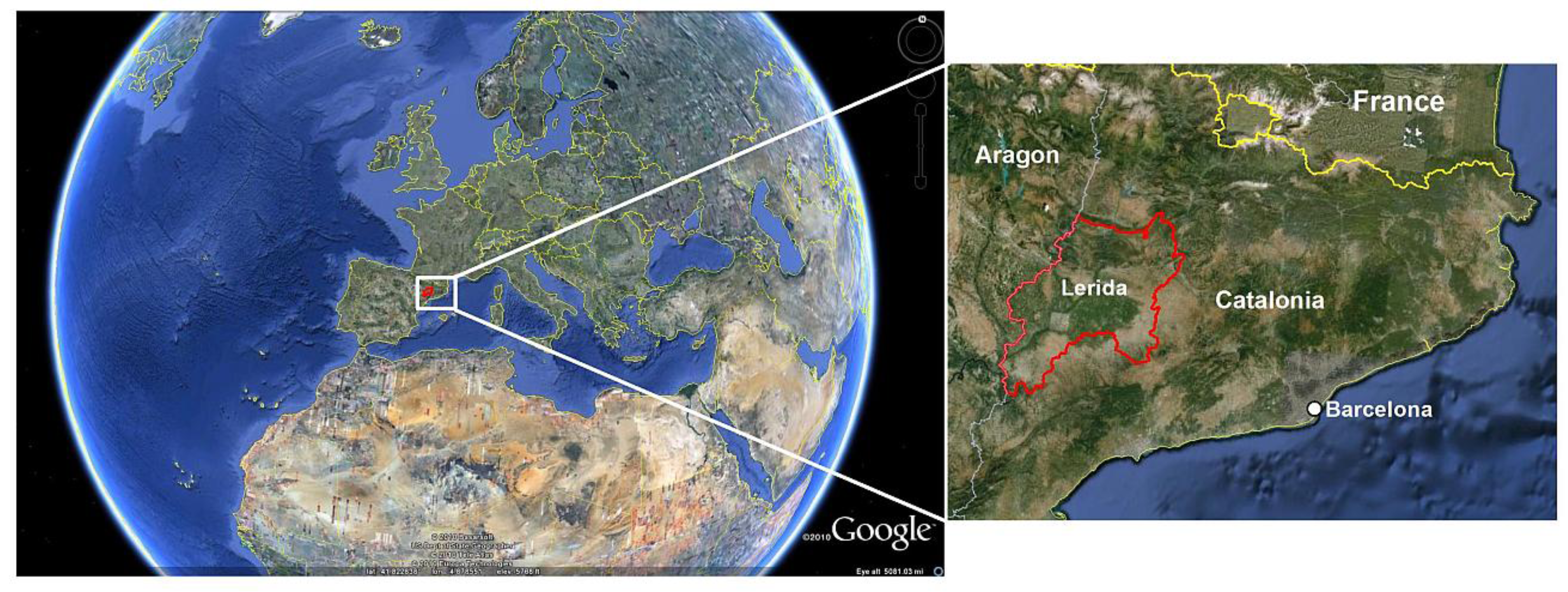
2. Study Area

3. Materials and Methods
3.1. Open Access Geospatial Data

| Band | Spatial Resolution (m) | Lower Limit (µm) | Upper Limit (µm) | Designation | Optical Domain |
|---|---|---|---|---|---|
| 1 | 30 | 0.45 | 0.52 | Blue | Visible |
| 2 | 30 | 0.52 | 0.60 | Green | Visible |
| 3 | 30 | 0.63 | 0.69 | Red | Visible |
| 4 | 30 | 0.77 | 0.90 | Near Infrared | Infrared |
| 5 | 30 | 1.55 | 1.75 | Shortwave Infrared | Infrared |
| 6 | 60 | 10.40 | 12.50 | Thermal Infrared | Thermal |
| 7 | 30 | 2.09 | 2.35 | Shortwave Infrared | Infrared |
3.2. Explanatory Variables
| CLC2000 Classes | Area in km2 | Percent of Study Area |
|---|---|---|
| Permanently irrigated land | 1,440 | 26.48 |
| Non-irrigated arable land | 1,182 | 21.74 |
| Complex cultivation patterns | 923 | 16.97 |
| Fruit trees and berry plantations | 452 | 8.31 |
| Agricultural with natural vegetation | 396 | 7.27 |
| Transitional woodland-shrub | 331 | 6.08 |
| Sclerophyllous vegetation | 240 | 4.41 |
| Broad-leaved forest | 240 | 4.41 |
| Mixed forest | 56 | 1.04 |
| Water bodies | 50 | 0.92 |
| Continuous urban fabric | 38 | 0.69 |
| Vineyards | 26 | 0.48 |
| Water courses | 16 | 0.29 |
| Olive groves | 12 | 0.23 |
| Natural grasslands | 8 | 0.15 |
| Industrial or commercial units | 8 | 0.14 |
| Discontinuous urban fabric | 5 | 0.10 |
| Mineral extraction sites | 5 | 0.09 |
| Bare rocks | 3 | 0.05 |
| Inland marshes | 2 | 0.04 |
| Annual crops associated with perm crops | 2 | 0.03 |
| Pastures | 1 | 0.02 |
| Rice fields | 1 | 0.02 |
| Sparsely vegetated areas | 1 | 0.02 |
| Sport and leisure facilities | 0.5 | 0.01 |
| Construction sites | 0.2 | 0.004 |
| Variable | Coefficient | S.E. | Wald | p | |
|---|---|---|---|---|---|
| Landsat ETM+ | Standard deviation ETM+1: BAND1SD | −1.106 | 0.636 | −1.74 | 0.009 |
| Standard deviation ETM+2: BAND2SD | 0.017 | 0.027 | 0.63 | 0.523 | |
| Standard deviation ETM+3: BAND3SD | 0.027 | 0.016 | 1.69 | 0.103 | |
| Standard deviation ETM+4: BAND4SD | 0.012 | 0.019 | 0.63 | 0.523 | |
| Standard deviation ETM+5: BAND5SD | −0.005 | 0.018 | −0.28 | 0.763 | |
| Standard deviation ETM+7: BAND7SD | 0.022 | 0.018 | 1.22 | 0.209 | |
| Coefficient of variation ETM+1: BAND1CV | 1.172 | 1.240 | 0.95 | 0.344 | |
| Coefficient of variation ETM+2: BAND2CV | 1.397 | 1.225 | 1.14 | 0.253 | |
| Coefficient of variation ETM+3: BAND3CV | 1.922 | 0.934 | 2.06 | 0.039 | |
| Coefficient of variation ETM+4: BAND4CV | −1.003 | 1.005 | −1.00 | 0.318 | |
| Coefficient of variation ETM+5: BAND5CV | −2.994 | 1.049 | −2.85 | 0.003 | |
| Coefficient of variation ETM+7: BAND7CV | 0.995 | 0.964 | 1.03 | 0.302 | |
| LST (°C) | 2.182 | 1.052 | 2.07 | <0.001 | |
| MSAVI | 2.311 | 0.677 | 3.41 | <0.001 | |
| SRTM | Digital elevation model: DEM (meters) | −0.001 | 0.007 | −0.15 | 0.022 |
| Slope: SLOPE (degrees) | −0.252 | 0.047 | −5.36 | 0.001 | |
| Aspect: ASPECT | −0.001 | 0.001 | −1.00 | 0.311 | |
| CLC2000 | Agricultural with natural vegetation: PANV * | −0.522 | 0.775 | −0.67 | 0.500 |
| Broad-leaved forest: BLF * | −2.453 | 0.895 | −2.74 | 0.206 | |
| Complex cultivation patterns: CCP * | −0.393 | 0.390 | −1.01 | 0.314 | |
| Fruit trees and berry plantations: FTBP * | −0.479 | 0.460 | −1.04 | 0.298 | |
| Non-irrigated arable land: NIAL * | 2.694 | 0.594 | 4.54 | <0.001 | |
| Permanently irrigated land: PIL * | 1.139 | 0.397 | 2.87 | 0.004 | |
| Sclerophyllous vegetation: SVEG * | −0.449 | 0.798 | −0.56 | 0.573 | |
| Transitional woodland-shrub: TWS * | −2.469 | 0.722 | −3.42 | 0.600 | |
| Distance to wet areas: WETDIST (meters) | 7.69e−5 | 1.95e−05 | 3.94 | <0.001 | |
| Distance to human activity: HUMDIST (meters) | −1.26e−04 | 3.74e−05 | −3.37 | <0.001 |
3.2.1. Satellite Image Texture (ETM+)
3.2.2. Vegetation Index (ETM+)
3.2.3. Land Surface Temperature (ETM+)
3.2.4. Landscape Metrics (CLC2000)
3.2.5. Topography (SRTM)
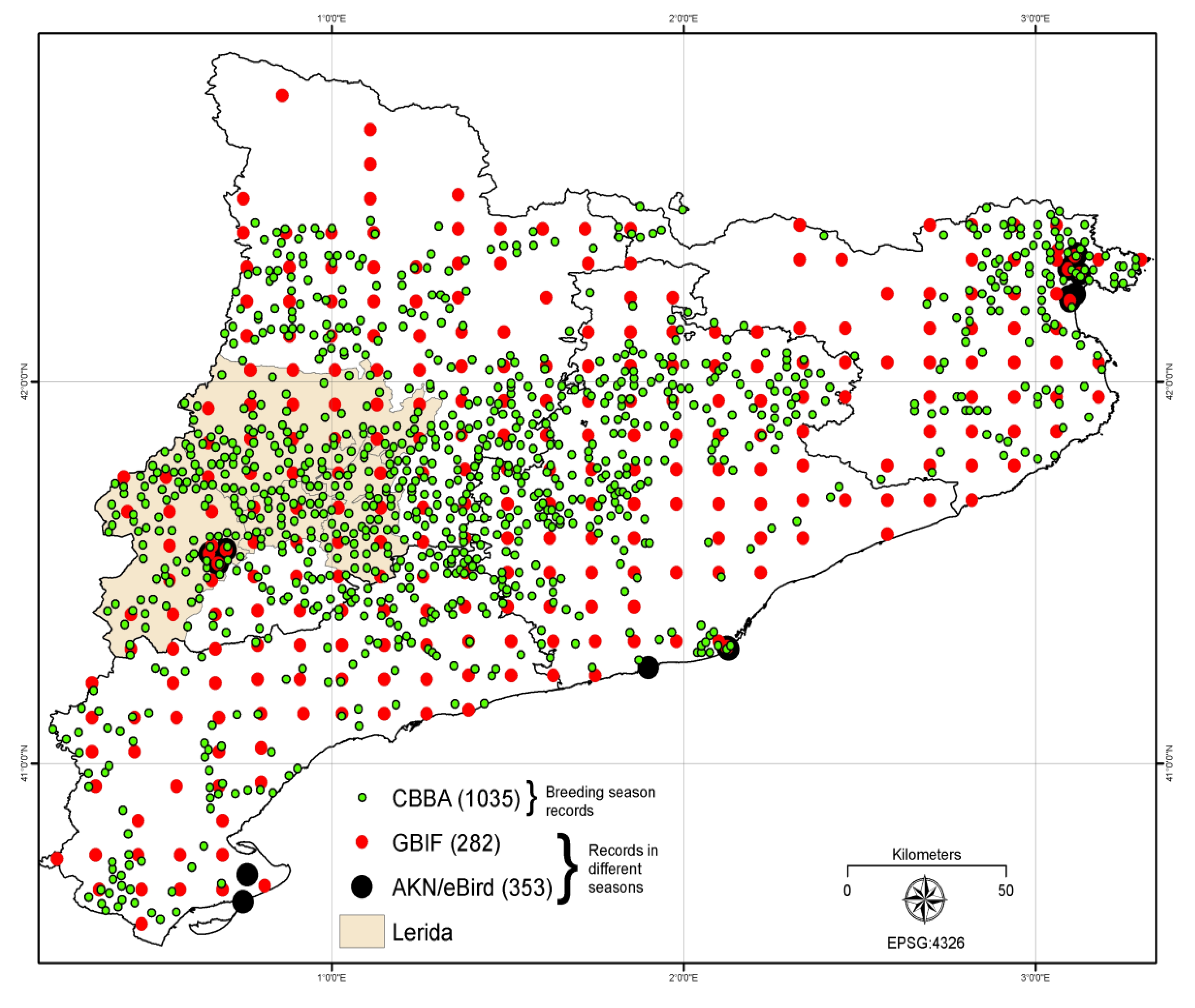
3.3. Open Access Bird Data

Data from the Catalan Breeding Bird Atlas
3.4. Free and Open Source Geospatial Software
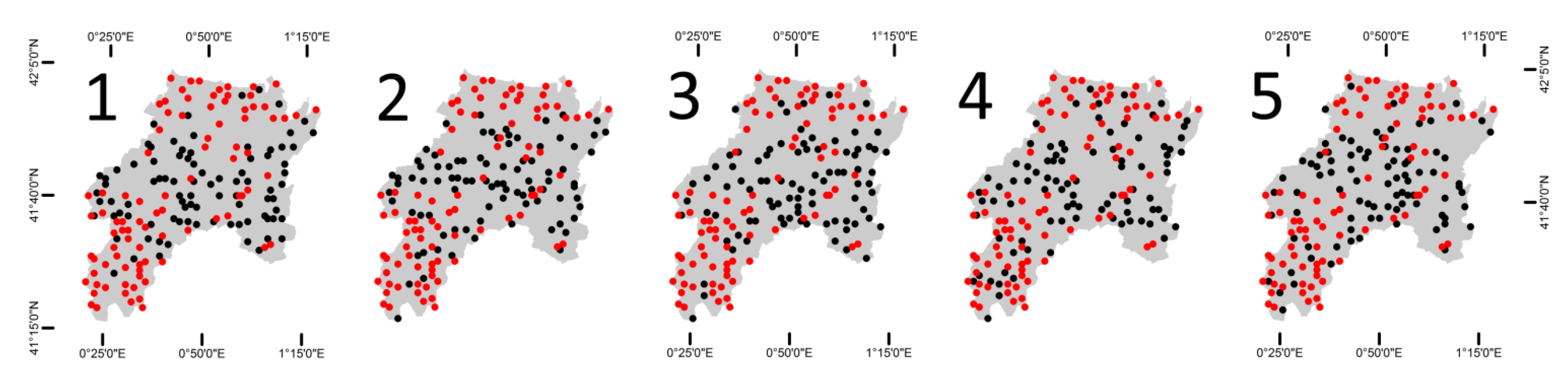
3.5. Modeling


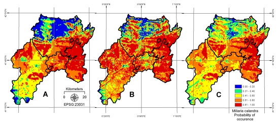
4. Results
| Variable | Coefficient | S.E. | Wald | p |
|---|---|---|---|---|
| (Intercept) | −0.703 | 0.456 | −1.542 | 0.123 |
| PANV | 1.207 | 0.861 | 1.402 | 0.161 |
| CCP | 1.136 | 0.539 | 2.108 | 0.035 |
| FTBP | 1.291 | 0.613 | 2.106 | 0.035 |
| NIAL | 4.032 | 0.721 | 5.592 | <0.001 |
| PIL | 2.395 | 0.557 | 4.300 | 0.002 |
| SVEG | 1.924 | 0.976 | 1.971 | 0.048 |
| HUMDIST | −8e−05 * | 5e05 ** | −1.6E−10 | 0.091 |
| WETDIST | −5e−05 | 2e05 | −2.501 | 0.016 |
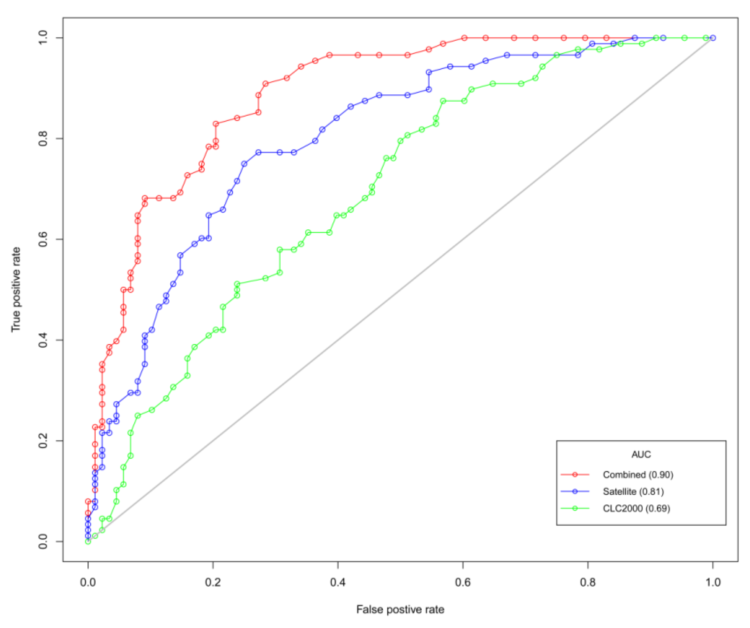
| AIC | 355 | AUC | 0.69 |
| Variable | Coefficient | S.E. | Wald | p |
|---|---|---|---|---|
| (Intercept) | −12.741 | 3.004 | −4.241 | 0.002 |
| MSAVI | 3.432 | 0.979 | 3.506 | <0.001 |
| BAND1SD | −0.093 | 0.056 | −1.661 | 0.097 |
| BAND5CV | 5.255 | 1.735 | 3.029 | 0.002 |
| DEM | 0.003 | 0.001 | 3.001 | 0.011 |
| SLOPE | −0.301 | 0.075 | −4.013 | <0.001 |
| LST | 0.286 | 0.071 | 4.028 | <0.001 |
| AIC | 310 | AUC | 0.81 |
| Variable | Coefficient | S.E. | Wald | p |
|---|---|---|---|---|
| (Intercept) | −12.16 | 3.495 | −3.479 | 0.005 |
| MSAVI (A) | 3.287 | 0.883 | 3.723 | 0.002 |
| LST (B) | 0.328 | 0.095 | 3.453 | <0.001 |
| BAND5CV (C) | 4.600 | 1.856 | 2.478 | 0.013 |
| BAND1SD (D) | −0.141 | 0.060 | −2.350 | 0.019 |
| SLOPE (E) | −0.211 | 0.082 | −2.573 | 0.010 |
| BLF (F) | −0.002 | 0.001 | −2.001 | 0.051 |
| NIAL (G) | 1.975 | 0.613 | 3.222 | 0.001 |
| PIL (H) | 1.658 | 0.685 | 2.420 | 0.015 |
| HUMDIST (I) | −9e−05 | 5e−05 | −1.801 | 0.048 |
| AIC | 285 | AUC | 0.90 |


5. Discussion
6. Conclusion
Acknowledgments
Conflict of Interest
References
- Birdlife-International. In Birds in the European Union: A Status Assessment, 1st ed.; Birdlife International: Wageningen, The Netherlands, 2004.
- Deceuninck, B. The Corncrake (Crex crex) in France; Schaeffer, N., Mammen, U., Eds.; International Corncrake Workshop: Hilpoltstein, Germany, 1998. [Google Scholar]
- De Leo, G.A.; Focardi, S.; Gatto, M.; Cattadori, I.M. The decline of the grey partridge in Europe: Comparing demographies in traditional and modern agricultural landscapes. Ecol. Model. 2004, 177, 313–335. [Google Scholar] [CrossRef]
- Tucker, G.M.; Heath, M.F. Birds in Europe: Their Conservation Status; BirdLife International: Cambridge, UK, 1994. [Google Scholar]
- Vepsäläinen, V.; Pakkala, T.; Piha, M.; Tiainen, J. Population crash of the ortolan bunting Emberiza hortulana in agricultural landscapes of southern Finland. Ann. Zoologici. Fennici 2005, 42, 91–107. [Google Scholar]
- Kosicki, J.Z.; Chylarecki, P. Habitat selection of the Ortolan bunting Emberiza hortulana in Poland: Predictions from large-scale habitat elements. Ecol. Res. 2012, 27, 347–355. [Google Scholar] [CrossRef]
- Evans, A.; Smith, K. Habitat selection of Cirl Buntings Emberiza cirlus wintering in Britain. Bird Study 1994, 41, 81–87. [Google Scholar] [CrossRef]
- Wotton, S.R.; Langston, R.H.W.; Gibbons, D.W.; Pierce, A.J. The status of the Cirl Bunting Emberiza cirlus in the UK and the Channel Islands in 1998. Bird Study 2000, 47, 138–146. [Google Scholar] [CrossRef]
- Stoate, C.; Moreby, S.J.; Szczur, J. Breeding ecology of farmland Yellowhammers Emberiza citrinella. Bird Study 1998, 45, 109–121. [Google Scholar] [CrossRef]
- Golawski, A.; Dombrowski, A. Habitat use of Yellowhammers Emberiza citrinella, Ortolan Buntings E. hortulana, and Corn Buntings Miliaria calandra in farmland of east-central Poland. Ornis Fennica 2002, 79, 164–172. [Google Scholar]
- Wretenberg, J.; Lindström, Å.; Svensson, S.; Pärt, T. Linking agricultural policies to population trends of Swedish farmland birds in different agricultural regions. J. Appl. Ecol. 2007, 44, 933–941. [Google Scholar] [CrossRef]
- Whittingham, M.J.; Swetnam, R.D.; Wilson, J.D.; Chamberlain, D.E.; Freckleton, R.P. Habitat selection by yellowhammers Emberiza citrinella on lowland farmland at two spatial scales: Implications for conservation management. J. Appl. Ecol. 2005, 42, 270–280. [Google Scholar] [CrossRef]
- Brickle, N.; Harper, D.; Aebischer, N.; Cockayne, S. Effects of agricultural intensification on the breeding success of corn buntings Miliaria calandra. J. Appl. Ecol. 2000, 37, 742–755. [Google Scholar] [CrossRef]
- Orlowski, G. Endangered and declining bird species of abandoned farmland in south-western Poland. Agric. Ecosyst. Environ. 2005, 111, 231–236. [Google Scholar] [CrossRef]
- Eisloeffel, F. The Corn Bunting (Miliaria calandra) in South-West Germany: Population Decline and Habitat Requirements. In The Ecology and Conservation of Corn Buntings (Miliaria calandra); Donald, P.F., Aebischer, N.J., Eds.; Joint Nature Conservation Committee: Peterborough, UK, 1997; pp. 170–173. [Google Scholar]
- Taylor, A.J.; O’Halloran, J. The decline of the Corn Bunting Miliaria calandra, in the Republic of Ireland. Biology Environ. Proc. Royal Irish Acad. 2002, 102, 165–175. [Google Scholar] [CrossRef]
- Donald, P.F.; Green, R.E.; Heath, M.F. Agricultural intensification and the collapse of Europe’s farmland bird populations. Proc. Royal Soc. B 2001, 268, 25–29. [Google Scholar] [CrossRef]
- Fuller, R.M.; Devereux, B.J.; Gillings, S.; Amable, G.S. Indices of bird-habitat preference from field surveys of birds and remote sensing of land cover: A study of south-eastern England with wider implications for conservation and biodiversity assessment. Global Ecol. Biogeogr. 2005, 14, 223–239. [Google Scholar] [CrossRef]
- Kuczynski, L.; Antczak, M.; Czechowski, P.; Grzybek, J.; Jerzak, L.; Zablocki, P.; Tryjanowski, P. A large scale survey of the great grey shrike Lanius excubitor in Poland: Breeding densities, habitat use and population trends. Ann. Zoologici Fennici 2010, 47, 67–78. [Google Scholar] [CrossRef]
- Diaz, M.; Telleria, J.L. Habitat Selection and Distribution Trends of Corn Buntings in the Iberian Peninsula. In The Ecology and Conservation of Corn Buntings Miliaria Calandra; Donald, P., Aebischer, N.J., Eds.; JNCC: Peterborough, UK, 1997; pp. 151–161. [Google Scholar]
- Stoate, C.; Borralho, R.; Araujo, M. Factors affecting corn bunting Miliaria calandra abundance in a Portuguese agricultural landscape. Agric. Ecosyst. Environ. 2000, 77, 219–226. [Google Scholar] [CrossRef]
- Brambilla, M.; Guidali, F.; Negri, I. Breeding-season habitat associations of the declining Corn Bunting Emberiza calandra—A potential indicator of the overall bunting richness. Ornis Fennica 2009, 86, 41–50. [Google Scholar]
- Brotons, L.; Manosa, S.; Estrada, J. Modelling the effects of irrigation schemes on the distribution of steppe birds in Mediterranean farmland. Biodivers. Conserv. 2004, 13, 1039–1058. [Google Scholar] [CrossRef]
- Moreno-Mateos, D.; Pedrocchi, C.; Comin, F.A. Avian communities’ presence in recently created agricultural wetlands in irrigated landscapes of semi-arid areas. Biodivers. Conserv. 2009, 18, 811–828. [Google Scholar] [CrossRef]
- Reeves, H.M.; Cooch, F.G.; Munro, R.E. Monitoring arctic habitat and goose production by satellite imagery. J. Wildl. Manag. 1976, 40, 532–541. [Google Scholar] [CrossRef]
- Cannon, R.W.; Knopf, F.L.; Pettinger, L.R. Use of Landsat data to evaluate Lesser Prairie Chicken habitats in western Oklahoma. J. Wildl. Manag. 1982, 46, 915–922. [Google Scholar] [CrossRef]
- Lauver, C.L.; Whistler, J. A hierarchical classification of Landsat TM imagery to identify natural grassland areas and rare species habitat. Photogramm. Eng. Remote Sens. 1993, 59, 627–634. [Google Scholar]
- Shirley, S.; Yang, Z.; Hutchinson, R.; Alexander, J.; McGarigal, K.; Betts, M. Species distribution modelling for the people: Unclassified landsat TM imagery predicts bird occurrence at fine resolutions. Divers. Distrib. 2013, 19, 855–866. [Google Scholar] [CrossRef]
- Houska, T.R.; Johnson, A.P. GloVis Ver. 8.17.1.; US Geological Survey General Information Product Series 137; Earth Resources Observation and Science (EROS) Center: Reston, VA, USA, 2012. [Google Scholar]
- Goslee, S.C. Analyzing remote sensing data in R: The Landsat package. J. Stat. Softw. 2011, 43, 1–25. [Google Scholar]
- R Development Core Team, R: A Language and Environment for Statistical Computing; R Foundation for Statistical Computing: Vienna, Austria, 2009.
- Rabus, B.; Eineder, M.; Roth, A.; Bamler, R. The shuttle radar topography mission—A new class of digital elevation models acquired by spaceborne radar. ISPRS J. Photogramm. Remote Sens. 2003, 57, 241–262. [Google Scholar] [CrossRef]
- Oliver, T.; Roy, D.B.; Hill, J.K.; Brereton, T.; Thomas, C.D. Heterogeneous landscapes promote population stability. Ecol. Lett. 2010, 13, 473–484. [Google Scholar] [CrossRef]
- Jarvis, A.; Reuter, H.; Nelson, A.; Guevara, E. Hole-Filled SRTM for the Globe Version 4. In CGIAR-CSI SRTM 90 m Database. Available online: http://srtm.csi.cgiar.org (accessed on 12 November 2009).
- Büttner, G.; Feranec, J.; Jaffrain, G.; Mari, L.; Maucha, G.; Soukup, T. The CORINE land cover 2000 project. EARSeL eProc. 2004, 3, 331–346. [Google Scholar]
- Saveraid, E.H.; Debinski, D.M.; Kindscher, K.; Jakubauskas, M.E. A comparison of satellite data and landscape variables in predicting bird species occurrences in the Greater Yellowstone Ecosystem, USA. Landsc. Ecol. 2001, 16, 71–83. [Google Scholar] [CrossRef]
- St-Louis, V.; Pidgeon, A.M.; Clayton, M.K.; Locke, B.A.; Bash, D.; Radeloff, V.C. Satellite image texture and a vegetation index predict avian biodiversity in the Chihuahuan Desert of New Mexico. Ecography 2009, 32, 468–480. [Google Scholar] [CrossRef]
- Horning, N.; Robinson, J.; Sterling, E.; Turner, W.; Spector, S. Remote Sensing for Ecology and Conservation; Oxford University Press: Oxford, UK, 2010; pp. 108–111. [Google Scholar]
- Qi, J.; Chehbouni, A.; Huete, A.R.; Kerr, Y.H.; Sorooshian, S. A modified soil adjusted vegetation index. Remote Sens. Environ. 1994, 48, 119–126. [Google Scholar] [CrossRef]
- Lambin, E.F.; Ehrlich, D. The surface temperature-vegetation index space for land cover and land-cover change analysis. Int. J. Remote Sens. 1996, 17, 463–487. [Google Scholar] [CrossRef]
- Quattrochi, D.A.; Luvall, J.C. Thermal infrared remote sensing for analysis of landscape ecological processes: Methods and applications. Landsc. Ecol. 1999, 14, 577–598. [Google Scholar] [CrossRef]
- Kerr, J.T.; Ostrovsky, M. From space to species: Ecological applications for remote sensing. Trends Ecol. Evol. 2003, 18, 299–305. [Google Scholar] [CrossRef]
- Sobrino, J.A.; Jiménez-Muñoz, J.C.; Paolini, L. Land surface temperature retrieval from Landsat TM 5. Remote Sens. Environ. 2004, 90, 434–440. [Google Scholar] [CrossRef]
- NASA, Band 6 Conversion to Temperature. In Landsat 7 Science Data Users Handbook; ational Aeronautics and Space Administration: Greenbelt, MD, USA, 2009; pp. 117–120.
- Gustafson, E.J.; Parker, G.R.; Backs, S.E. Evaluating spatial pattern of wildlife habitat: A case study of the wild Turkey (Meleagris gallopavo). Am. Midl. Nat. 1994, 131, 24–33. [Google Scholar] [CrossRef]
- Fauth, P.T.; Gustafson, E.J.; Rabenold, K.N. Using landscape metrics to model source habitat for Neotropical migrants in the Midwestern US. Landsc. Ecol. 2000, 15, 621–631. [Google Scholar] [CrossRef]
- De Smith, M.J.; Goodchild, M.F.; Longley, P.A. Grid-based Statistics. In Geospatial Analysis: A Comprehensive Guide to Principles, Techniques and Software Tools; Troubador Publishing Ltd.: Leicester, UK, 2007; pp. 194–199. [Google Scholar]
- Vander Haegen, W.M.; Dobler, F.C.; Pierce, D.J. Shrubsteppe bird response to habitat and landscape variables in Eastern Washington, USA. Conserv. Biol. 2000, 14, 1145–1160. [Google Scholar] [CrossRef]
- Edwards, J.L.; Lane, M.A.; Nielsen, E.S. Interoperability of biodiversity databases: Biodiversity information on every desktop. Science 2000, 289, 2312–2314. [Google Scholar] [CrossRef]
- Sullivan, B.L.; Wood, C.L.; Iliff, M.J.; Bonney, R.E.; Fink, D.; Kelling, S. eBird: A citizen-based bird observation network in the biological sciences. Biol. Conser. 2009, 142, 2282–2292. [Google Scholar] [CrossRef]
- Brotons, L.; Herrando, S.; Estrada, J.; Pedrocchi, V.; Martin, J.L. The Catalan Breeding Bird Atlas (CBBA): Methodological aspects and ecological implications. Revista Catalana d’Ornitologia 2008, 24, 118–137. [Google Scholar]
- Keitt, T.H.; Bivand, R.; Pebesma, E.; Rowlingson, B. Rgdal: Bindings for the Geospatial Data Abstraction Library. R Package Version 0.6–25. 2010. Available online: http://cran.r-project.org/web/packages/rgdal/index.html (accessed on 25 February 2010),.
- Lindsay, J. Whitebox Geospatial Analysis Tools; Department of Geography, University of Guelph: Guelph, Ontario, Canada, 2009. Available online: Available online: http://www.uoguelph.ca/~hydrogeo/ Whitebox/ (accessed on 29 December 2009).
- Cimmery, V. User Guide for SAGA. Version 2.0, 2007. Available online: http://saga-gis.org/ (accessed on 15 January 2010).
- Gagné, M. Moving to Ubuntu Linux; Pearson Education: Upper Saddle River, NJ, USA, 2006. [Google Scholar]
- Hosmer, D.W.; Lemeshow, S. Applied Logistic Regression, 2nd ed.; John Wiley & Sons, Inc.: New York, NY, USA, 2000. [Google Scholar]
- Akaike, H. Information Theory as an Extension of the Maximum Likelihood Principle; Petrov, B.N., Csaki, F., Eds.; Akademiai Kiado: Budapest, Hungary, 1973; pp. 267–281. [Google Scholar]
- Brauner, N.; Shacham, M. Role of range and precision of the independent variable in regression of data. Am. Inst. Chem. Eng. J. 1998, 44, 603–611. [Google Scholar] [CrossRef]
- O’Brien, R.M. A caution regarding rules of thumb for variance inflation factors. Qual. Quantity 2007, 41, 673–690. [Google Scholar] [CrossRef]
- Cohen, J. A coefficient of agreement for nominal scales. Educ. Psychological Meas. 1960, 20, 37–46. [Google Scholar] [CrossRef]
- Deleo, J.M. Receiver Operating Characteristic Laboratory (ROCLAB): Software for Developing Decision Strategies that Account for Uncertainity. In Proceedings of Second International Symposium on Uncertainty Modelling and Analysis, College Park, MD, 25–28 April 1993; IEEE Computer Society Press: College Park, MD, USA, 1993; pp. 318–325. [Google Scholar]
- Baraldi, A.; Parmiggiani, F. An investigation of the textural characteristics associated withgray level cooccurrence matrix statistical parameters. IEEE Trans. Geosci. Remote Sens. 1995, 33, 293–304. [Google Scholar] [CrossRef]
- Seoane, J.; Bustamante, J.; Diaz-Delgado, R. Competing roles for landscape, vegetation, topography and climate in predictive models of bird distribution. Ecol. Model. 2004, 171, 209–222. [Google Scholar] [CrossRef]
- Carrao, H.; Caetano, M. The Effect of Scale on Landscape Metrics. In Proceedings of International Symposium of Remote Sensing of the Environment, Buenos Aires, Argentina, 8–12 April 2002.
- Whited, D.; Galatowitsch, S.; Tester, J.R.; Schik, K.; Lehtinen, R.; Husveth, J. The importance of local and regional factors in predicting effective conservation: Planning strategies for wetland bird communities in agricultural and urban landscapes. Landsc. Urban. Plann. 2000, 49, 49–65. [Google Scholar] [CrossRef]
- Martí-Ragué, X.; Lescrauwaet, A.-K.; Borg, M.; Valls, M. Indicators Guidelines: To Adopt an Indicators-Based Approach to Evaluate Coastal Sustainable Development; Government of Catalonia: Barcelona, Spain, 2007. [Google Scholar]
- Seoane, J.; Bustamante, J.; Diaz-Delgado, R. Are existing vegetation maps adequate to predict bird distributions? Ecol. Model. 2004, 175, 137–149. [Google Scholar] [CrossRef]
Appendix
| Explanatory Variable | VIF |
|---|---|
| MSAVI | 3.820 |
| BAND1SD | 0.095 |
| BAND5CV | 2.850 |
| SLOPE | 0.165 |
| LST | 0.283 |
| BLF | 0.438 |
| NIAL | 2.061 |
| PIL | 2.051 |
| HUMDIST | 4.3e−5 |
© 2013 by the authors; licensee MDPI, Basel, Switzerland. This article is an open access article distributed under the terms and conditions of the Creative Commons Attribution license (http://creativecommons.org/licenses/by/3.0/).
Share and Cite
Abdi, A.M. Integrating Open Access Geospatial Data to Map the Habitat Suitability of the Declining Corn Bunting (Miliaria calandra). ISPRS Int. J. Geo-Inf. 2013, 2, 935-954. https://doi.org/10.3390/ijgi2040935
Abdi AM. Integrating Open Access Geospatial Data to Map the Habitat Suitability of the Declining Corn Bunting (Miliaria calandra). ISPRS International Journal of Geo-Information. 2013; 2(4):935-954. https://doi.org/10.3390/ijgi2040935
Chicago/Turabian StyleAbdi, Abdulhakim M. 2013. "Integrating Open Access Geospatial Data to Map the Habitat Suitability of the Declining Corn Bunting (Miliaria calandra)" ISPRS International Journal of Geo-Information 2, no. 4: 935-954. https://doi.org/10.3390/ijgi2040935
APA StyleAbdi, A. M. (2013). Integrating Open Access Geospatial Data to Map the Habitat Suitability of the Declining Corn Bunting (Miliaria calandra). ISPRS International Journal of Geo-Information, 2(4), 935-954. https://doi.org/10.3390/ijgi2040935