
Within Skyline Query Processing in Dynamic Road Networks


Department of Maritime Information and Technology, National Kaohsiung Marine University, Kaohsiung City 80543, Taiwan
ISPRS Int. J. Geo-Inf. 2017, 6(5), 137; https://doi.org/10.3390/ijgi6050137
Submission received: 22 January 2017
/
Revised: 26 April 2017
/
Accepted: 27 April 2017
/
Published: 29 April 2017
Abstract
:The continuous within skyline query is an important type of location-based query, which can provide useful skyline object information for the user. Previous studies on processing the continuous within skyline query focus exclusively on a static road network, where the object attributes and the conditions of roads remain unchanged. However, in real-world applications, object attributes and road conditions inevitably vary with time, which severely limits the applicability of previous studies in practice. Therefore, in this paper, we address the issue of efficiently processing the continuous within skyline query in dynamic road networks with time-varying information. We design three elaborate data structures, the object attribute dominating matrix (OADM), the road distance sorted list (RDSL) and the skyline object expansion tree (SOET), to maintain the information of objects and the road network. Combined with OADM, RDSL and SOET, we develop an efficient algorithm, namely the within skyline object updating algorithm, to provide real-time processing of the time-varying information. Finally, a thorough experimental evaluation is conducted to show the merits of the proposed approaches.
1. Introduction
With the fast advance of positioning techniques in mobile systems and the popularization of portable computers (e.g., laptops, 3G mobile phones and tablet PCs), spatio-temporal databases that aim at efficiently managing a large number of moving objects so as to support various types of location-based queries have attracted much attention in the database community [1,2,3,4]. Many applications, such as geographical information systems, traffic control systems and location-aware advertisements, can benefit from efficient processing of the location-based queries. The distance-based skyline query is an important type of location-based query that can provide useful information for preference-based data analysis and has a wide range of real applications [5,6,7]. Given a set of data objects with m dimensional attributes and a query object q in a road network, the distance-based skyline query finds the objects in that are not dominated by any other object, in terms of the m attributes and the road distance to q. More specifically, object p dominates another object if (1) its value in each attribute is as good or better than that of and is better in at least one attribute and (2) it is closer to q than . The objects not dominated by others are termed the skyline objects.
A novel distance-based skyline query, called the within skyline query, can be used to find the skyline objects within a given distance range, where the objects retrieved are termed the within skyline objects (WSOs). In the previous work [8], the continuous within skyline query is presented for continuous monitoring of WSOs in road networks. Given a path , along which the query object q moves, a set of data objects and a distance d, the continuous within skyline query finds a set of WSOs for each point p on , such that the road distance from each WSO to point p is less than or equal to d. The continuous within skyline query can be found in many fields and application domains. A real-world example is that of a traveler who is planning a trip, who may want to know which hotels are better to stay at en route. In this scenario, the traveler can issue the continuous within skyline query to find the hotels within the distance range d and with good quality (e.g., higher rank and lower price) during the trip.
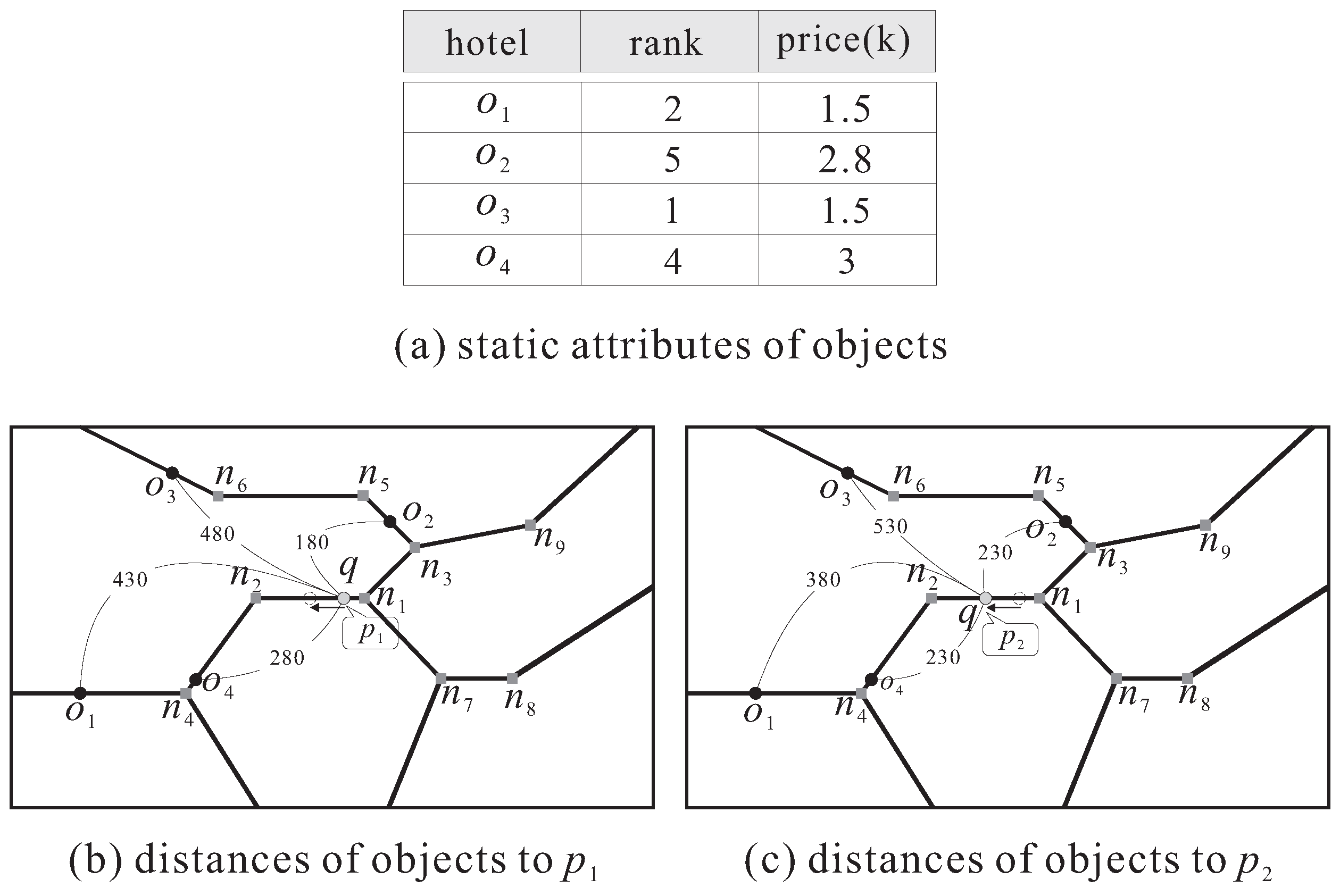
Figure 1 illustrates an example of processing the continuous within skyline query, where objects to and the query object q are located in a road network, represented as a graph consisting of nodes and edges. Figure 1a shows the static attributes (i.e., “rank” and “price”) of the four objects. In this example, the query object q moves from node to node (that is, the query path is ). Assume that the continuous within skyline query is issued to find the WSOs whose road distances to q are within 300 (i.e., ). When q is located at point (as shown in Figure 1b), only object is the WSO. Note that although is not dominated by , it cannot be the WSO because its road distance to q is greater than d. When q moves to point (as shown in Figure 1c), the road distance of object to is equal to that of object . That is, when q is located at the left side of , object becomes closer to q than . Thus, is better than in the “distance” dimension, so that becomes a skyline object. As the road distances of and are both less than d, they are the WSOs.
The processing techniques for the continuous within skyline query developed in [8] focus exclusively on a static road network, where the information of objects (i.e., their object attributes) and the conditions of roads remain unchanged. However, in real-world applications, object information and road conditions inevitably vary with time. For example, a hotel offers a discount so as to attract more customers (that is, varying the “price” attribute), and a crash obstructs the road for several hours (in this case, the length of the road is changed to ∞). Such varying information about objects and roads may outdate the previous query result, so that the continuous within skyline query needs to be evaluated again. This incurs the problem of high re-evaluation cost, which severely limits the applicability of the approaches in [8] in practice.
In this paper, we address the issue of efficiently processing the continuous within skyline query in dynamic road networks with time-varying information, where three types of time-varying information are taken into account. The first type of time-varying information is the time-varying object attribute, in which an object o changes its attribute from to . The second type is the time-varying edge length, where the length of an edge e changes from to ∞ (meaning that the road is temporarily closed) or from ∞ to (i.e., the road now is passable). The last one is the time-varying query path, where the query path has been changed to because there are road congestions or accidents on the roads in .
To provide real-time processing of the above time-varying information, we need to quickly examine whether the WSOs of the continuous within skyline query are affected by the time-varying information and then evaluate the new WSOs if necessary. Therefore, we design three elaborate data structures, the object attribute dominating matrix (OADM), the road distance sorted list (RDSL) and the skyline object expansion tree (SOET), to adequately maintain the information of objects and the road network, which can be used to facilitate the task of quickly determining which time-varying information influences the query result. Moreover, we develop an efficient algorithm, namely the within skyline object updating algorithm, combined with the three data structures to rapidly evaluate the new result of the continuous within skyline query. For better readability, Table 1 summarizes the notations used.
The main contributions of this paper are summarized as follows.
- We address the issue of efficiently processing the continuous within skyline query in dynamic road networks, where three types of time-varying information, the time-varying object attribute, the time-varying edge length and the time-varying query path, are taken into account in query processing.
- Three data structures, OADM, RDSL and SOET, are designed to adequately maintain the information of objects and the road network, in order to efficiently handle the time-varying information.
- We propose the within skyline object updating algorithm, combined with the three data structures, to rapidly evaluate the new query result affected by the time-varying information.
- A comprehensive set of experiments is conducted to demonstrate the merits of the proposed approaches.
The remainder of this paper is organized as follows. Section 2 reviews some related works. In Section 3, we present the three data structures, SADM, RDSL and SOET. Section 4 illustrates how the within skyline object updating algorithm works. Section 5 shows extensive experiments on the performance of the proposed methods. Finally, Section 6 concludes the paper with directions on future work.
2. Related Works
The skyline query is first studied in the area of computational geometry [9,10,11,12,13]. Several processing methods have been proposed to solve the continuous skyline query in Euclidean spaces. Cheema et al. [14] study the problem of continuously monitoring a moving skyline query by using a safe zone-based approach. Zheng et al. [15] propose continuous skyline computation over an incremental motion model, where the query point moves incrementally in discrete time steps with no restrictions and predictability. Vu et al. [16] further address the issue of processing the skyline query for object data with uncertainty.
In recent years, processing skyline queries in road networks has received considerable attention. Deng et al. [17] extend the concept of the spatial skyline [7] to road networks and present the multi-source skyline query (MSQ). Given a set of m query objects and a set of n data objects in a road network, each data object o is mapped to an m-dimensional point, where the value of the i-th dimension refers to the road distance between o and the i-th query object. Then, MSQ retrieves the skyline points that are not dominated in terms of the m dimensions. Deng et al. propose three algorithms, the Euclidean distance constraint (EDC), the lower bound constraint (LBC), and collaborative expansion (CE), to solve the MSQ problem. To improve the search performance, EDC and LBC utilize Euclidean distance as the lower bound of road distance to prune data objects. As for CE, the pruning strategy is to start from the m query objects to search the road network for candidate skyline objects. Once an object has been visited m times, those objects that have never been visited can be pruned. However, these algorithms may generate too many candidates and cause unnecessary road distance computation. Hence, Zou et al. [18] propose the shared shortest path (SSP) algorithm associated with the shortest path tree (SP-Tree) to overcome the problems. The criteria for determining the skyline points in the above methods are based on the road distances between data objects and query objects. Other studies [19,20] consider the skyline problem in multi-cost transportation networks (MCN), where each edge (i.e., road segment) is associated with multiple cost values and the skyline points are determined based on these cost values. Huang et al. [21] study another skyline problem of finding the skyline points that are not dominated in terms of only two attributes: (1) their network distance to a query location q and (2) the detour distance from q’s predefined route on the road network. Jang et al. [22] address the issue of processing continuous skyline queries in road networks. The idea is to pre-compute a range R for each data object o such that if the query object is within R, then o must be a skyline point in terms of its road distance to the query object and object attribute. Then, the skyline points of the query object can be determined based on the pre-computed ranges of all data objects. However, two major problems limit the applicability of this method. The first problem is that pre-computing all object ranges incurs tremendous processing cost, especially for a road network with a large size. The second is that the skyline result cannot provide useful information to the user because the skyline points far away from the query object are also included in the query result. Recently, Huang et al. [8] propose several approaches to process the continuous within skyline query in a static road network. For each edge , the procedure includes: (1) obtaining a set of global within skyline objects (GWSO) such that object must be a WSO for point p on edge e; and (2) determining some points on edge e such that the WSOs between two consecutive points remain the same and finding the corresponding WSOs of these points. However, as discussed in the Introduction, the time-varying information limits the applicability of their approach in practice.
The related works mentioned above focus exclusively on: (1) processing the skyline queries in Euclidean spaces (e.g., [14,15]), where the distance between objects is computed by simply using the objects’ locations rather than based on the connectivity of the road network; (2) answering the traditional skyline queries and their variants in the road networks (e.g., [7,17,18]); or (3) considering the continuous skyline query processing in a static road network (e.g., [8,22]), in which the information of objects and the conditions of the roads remain unchanged. In this paper, our efforts are devoted to overcoming the limitations of the previous works. That is, we investigate the continuous skyline problem in dynamic road networks with time-varying information.
3. Data Structures
The approach in [8] first determines a set GWSO for each edge and then finds the WSOs for point p on edge e by taking into consideration the objects in GWSO only. The set GWSO is represented as a union of the WSOs of the two nodes connected by the edge e and the objects on e, where determining the WSOs of the nodes dominates the overall performance of processing the continuous within skyline query since it involves a large number of road distance computations. To efficiently process the continuous within skyline query in dynamic road networks with time-varying information, we design three data structures, the object attribute dominating matrix (OADM), the road distance sorted list (RDSL) and the skyline object expansion tree (SOET), to maintain the information of objects and the road network. Benefiting from the data structures, we can quickly update the set GWSO for each edge affected by the time-varying information. In the following, we describe separately the three data structures in detail and discuss how to update them for the time-varying information (i.e., the time-varying object attribute, the time-varying edge length and the time-varying query path).
3.1. Object Attribute Dominating Matrix
For each node n belonging to the query path , the object attribute dominating matrix (OADM), represented as a 2D matrix, is designed to maintain the dominance relationships between objects, in terms of their object attributes. When the continuous within skyline query is processed, the rows and the columns of the OADM correspond to the objects whose road distances to n are less than or equal to the distance d. The reason why only such objects are kept in the OADM is that if their dominance relationships have been changed by the time-varying object attributes, the WSOs of node n could be affected. In other words, the time-varying object attributes of the objects not in the OADM cannot affect n’s WSOs.
In the OADM, the value of each entry is represented as follows:
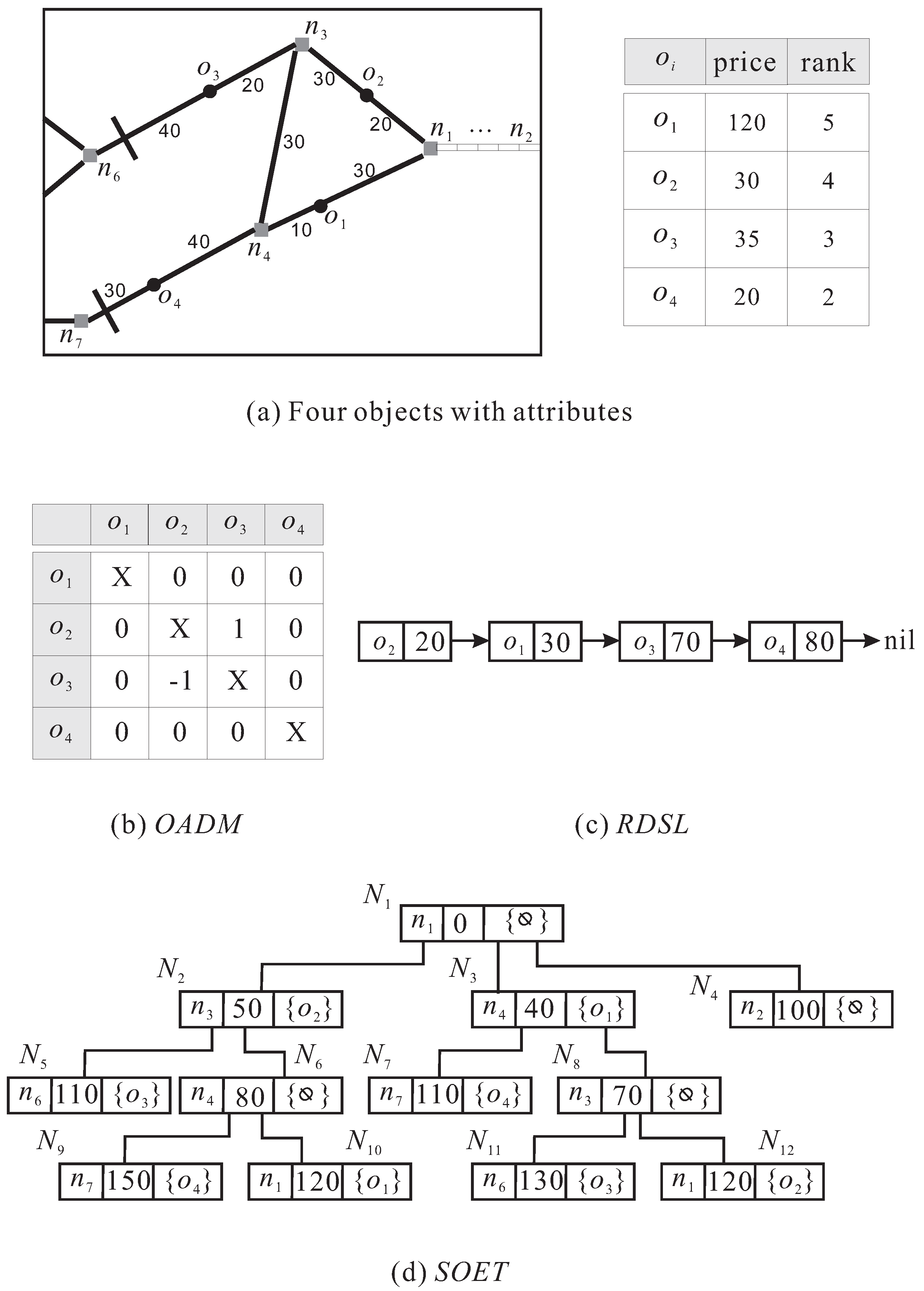
where “1” and “” mean that there is a dominance relationship between objects and , and “0” shows that and cannot dominate each other, in terms of their object attributes. Consider the example in Figure 2a, where four objects to are located on a road network, and have “price” and “rank” attributes. Assume that a continuous within skyline query is processed to find the skyline objects within the distance range . As the road distances between objects to and the node are less than or equal to 100, they all are kept in the OADM of . In terms of the “price” and “rank” attributes of objects, the value of each entry in the OADM can be determined by using Equation (1), as shown in Figure 2b. In this figure, only objects , and are the WSOs of node (because is dominated by ).
When the time-varying information (i.e., the time-varying object attribute, the time-varying edge length or the time-varying query path) has been changed, the OADM of node n needs to be updated accordingly, as discussed in the following.
- For the time-varying object attribute of an object o where o’s attribute is changed from to : if object o appears in the OADM, then the dominance relationships between o and the other objects in the OADM are re-checked based on , so as to update the values of entries in the row and the column containing o. Otherwise, the OADM need not be updated as o does not appear in the OADM.
- For the time-varying edge length of an edge e where the length of e is changed from to ∞ (or ∞ to ): in the case that e’s length is changed from to ∞, the road distances of some objects to n would increase. Conversely, changing e’s length from ∞ to would decrease some objects’ road distances. As a result, the objects whose road distances updated by the time-varying edge length are less (greater) than or equal to d need to be added into (removed from) the OADM. Then, the values of new entries in the OADM are determined using Equation (1).
- For the time-varying query path where the query path is changed to : if the edge e connecting node n belongs to , then the OADM of n is still usable because e is not affected by the time-varying query path. Otherwise, e belongs to , and thus, the OADM of n is removed as n is not on the query path.
3.2. Road Distance Sorted List
As the road distance between each object and the query object plays an important role in determining the WSOs result, we design the road distance sorted list (RDSL) to store, for each node n belonging to the query path , the objects in ascending order of their road distances to n. Similar to the OADM, only the objects whose road distances to n do not exceed the distance d are stored in the RDSL. If the position of an object o in the RDSL is in front of that of another object , then o has a chance to dominate because of its smaller distance to n. Consider again Figure 2a, where objects to are within the distance range . According to their road distances to node , the RDSL of is shown in Figure 2c. In this figure, the entry in the OADM is equal to one (refer to Figure 2b), and is in front of in the RDSL. Therefore, is dominated by in terms of “price”, “rank” and “distance” attributes. Note that although is not a WSO, it is still kept in the OADM and the RDSL because its distance to does not exceed d.
Due to the time-varying information, the road distances of objects in the RDSL of node n could be changed, as well as the order of objects. Once the RDSL is affected by the time-varying object attribute, the time-varying edge length or the time-varying query path, it needs to be updated as follows.
- For the time-varying object attribute of an object o: changing o’s attribute from to affects only the dominance relationship between o and the other objects, in terms of object attributes. The road distances of objects to node n remain unchanged so that the order of objects in the RDSL is not affected by the time-varying object attribute.
- For the time-varying edge length of an edge e: if the length of e is changed from to ∞ (i.e., e is temporarily closed), then the distances of some objects to n increase. For each object in the RDSL of n, once its road distance affected by e is greater than d, it needs to be removed. In the case that e’s length is changed from ∞ to , some objects would have decreasing distances to n because e is now passable. Therefore, such objects can be added into the RDSL if their decreasing distances do not exceed d. In addition to increasing or decreasing the road distance of the object, the time-varying edge length of e may also result in an adjustment in the order of objects in the RDSL.
- For the time-varying query path where the query path is changed to : similar to the process of updating the OADM of node n mentioned in Section 3.1, the RDSL of n is removed only if n is not on the new query path .
3.3. Skyline Object Expansion Tree
As discussed in the previous subsections, the time-varying edge length of an edge e results in the re-computations of the road distances of objects. However, computing the object distance by re-executing Dijkstra’s algorithm or the A* algorithm, whenever the time-varying edge length is changed, would incur high cost in processing the continuous within skyline query. In order to greatly reduce the computation cost, the skyline object expansion tree (SOET) is designed to quickly compute the road distances of objects affected by the time-varying edge length, without the need to execute the specific algorithms.
For each node n belonging to the query path , the SOET is built to keep information of the objects and the network nodes whose road distances to n are less than or equal to d. Then, by traversing the SOET, we can determine whether the time-varying edge length affects the objects within the distance range d and compute their new road distances to n if necessary. In the SOET, each tree node N has the structure , where refers to the network node id, is the road distance of to n, is the set of objects on the edge connecting and (where belongs to N’s parent node) and are the pointers to N’s child nodes. For ease of exposition, the road network presented in Figure 2a is used again to illustrate the SOET structure, where the distance region starts at the node and ends at the vertical marks with distance . Initially, the root of the SOET stores the start node ’s information, including the network node id , the distance to (i.e., 0) and . As node ’s adjacent nodes , and in the road network have the distances less than or equal to 100, the tree nodes , and in the forms of , and , respectively, are stored in the SOET and pointed by (i.e., they are the child nodes of ). Then, consider the adjacent nodes and of in the road network. Because the distances of object and node to do not exceed 100, the tree nodes and of the SOET are represented as and , respectively, and pointed by . Similarly, the tree nodes and in the forms of and , respectively, are the child nodes of . The corresponding SOET of node , consisting of 12 tree nodes to , is shown in Figure 2d. In the following, we discuss how to update the SOET of each node n when the time-varying information is changed.
- For the time-varying object attribute of an object o: for the continuous within skyline query, the SOET of n remains valid regardless of the time-varying object attribute, because of the unchanged distance d.
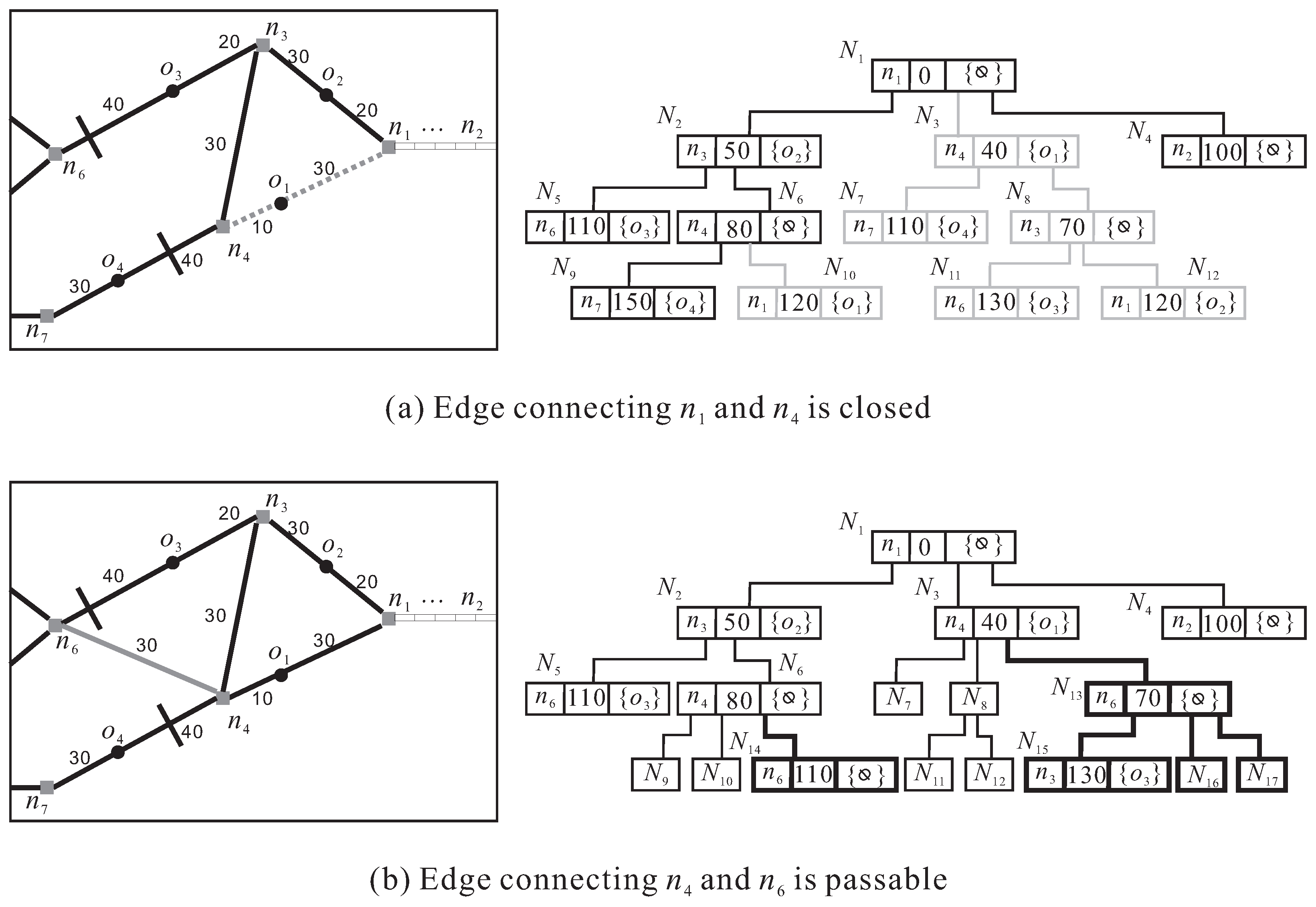
- For the time-varying edge length of an edge e: the process of updating the SOET of node n needs to first determine which objects are affected by e and then re-compute their road distances to n. For the case that the length of edge e connecting nodes and is changed from to ∞ (i.e., e is temporarily closed), the SOET of node n is traversed from its root down to leaf level so as to check whether there are parent-child relationships between the tree nodes containing and . If no such parent-child relationship exists, then the SOET of n remains valid because edge e connecting and falls out of the distance range d. Otherwise, the subtrees rooted at the tree nodes containing and are affected by e and need to be removed from the SOET. For the case that the length of edge e connecting nodes and is changed from ∞ to , some objects’ road distances can further decrease because e now is passable. As such, we perform a grown expansion starting from and to include the objects whose decreasing distances are less than or equal to d. Then, the subtree rooted at the tree node containing (or ) is updated accordingly to contain information of such objects. Here, we explain the two cases using a concrete example, continuing the previous example in Figure 2. Assume that the edge connecting nodes and is temporarily closed (corresponding to the first case), as shown in Figure 3a. Having traversed the SOET of node , we know that both the tree nodes and ( and ) contain node (). As there is a parent-child relationship between and ( and ), the subtree rooted at () is removed from the SOET (the shaded part in Figure 3a), so that the road distances of objects and are re-computed as ∞ (because is on e) and 120, respectively. As a result, objects and are removed from the OADM and the RDSL of . Going back to the example in Figure 2, assume that the edge connecting nodes and is passable, and its length is equal to 30 (corresponding to the second case), as shown in Figure 3b. Starting from the tree nodes and containing node , two new subtrees have been included into the SOET (the bold part in Figure 3b) because their updated distances do not exceed the distance 100.
- For the time-varying query path where the query path is changed to : if the node n is not on the new query path , then the SOET of n is removed.
4. Within Skyline Object Updating Algorithm
Recall that the WSOs result for each edge is obtained from the set , which is a union of the WSOs of the two nodes connected by e and the objects on e. Here, we denote the WSOs set of node n as . Determining the dominates the overall performance of processing the continuous within skyline query because it involves a large number of road distance computations. As the time-varying information (including the time-varying object attribute, the time-varying edge length and the time-varying query path) can potentially outdate the previous , it needs to be updated if necessary. An intuitive method to update the of node n is to re-execute the approach in [8] whenever the time-varying information is changed, which, however, would suffer from a long re-computation time for a large amount of time-varying information changed. Therefore, we develop the within skyline object updating algorithm to provide real-time processing of the time-varying object attribute, the time-varying edge length and the time-varying query path, so as to quickly update the of each node n on without the need to execute the approach in [8].
For the set of each node n on , the procedure of the within skyline object updating algorithm can be divided into three cases according to the type of time-varying information. The first case is that the time-varying information is changed by an object o (which may or may not be a WSO of n); the second one is that the time-varying information is changed by an edge e (that is, e is temporarily closed or now passable); and the last case is that the time-varying information corresponds to the time-varying query path (due to the road congestions or accidents on some roads belonging to ). In the following, we discuss the three cases separately.
4.1. Processing of Time-Varying Object Attribute
The main idea of processing the time-varying object attribute is to (1) determine whether the time-varying object attribute of object o affects the by examining whether o appears in the OADM and the RDSL of n and (2) update the by checking the value of entry in the OADM and the order of objects in the RDSL with respect to o. Suppose that object o changes its attribute from to . If o does not appear in the OADM and the RDSL of n, then the of node n need not be updated regardless of object o’s new attribute . This is because o falls outside the distance range d, and thus, the time-varying object attribute of o can be ignored. Otherwise (i.e., object o appears in the OADM and the RDSL), the dominance relationship between o and another object, say , may be changed by (that is, the values of entries and in the OADM have been modified), so that the previous needs to be further verified. According to whether o and are contained in the (i.e., they are the WSOs of n), the process of updating the can be divided into four cases: (1) and , (2) but , (3) , but , and (4) and , which are separately discussed in the following.
The first case where and implies that no object can dominate o and in terms of the object attributes and the “distance” attribute (closer to n than o and ). Let us observe the value of entry in the OADM affected by the time-varying object attribute, consisting of the following six conditions, to determine whether the needs to be updated.
- is changed from to zero: this means that there is no longer a dominance relationship between o and (i.e., o and cannot dominate each other). Because o and are still contained in the , changing from –0 cannot affect the and can be ignored.
- is changed from one to zero: same as the first condition, the is not affected even though is changed to zero.
- is changed from to one: o now can dominate in terms of the object attributes. Note that since o is previously dominated by in terms of the object attributes (), but still can be a WSO, o must be closer to n than (i.e., o is in front of in the RDSL). Therefore, when , needs to be removed from the .
- is changed from one to : similar to the third condition, o has to be removed from the because it is dominated by in terms of the object attributes and the “distance” attribute.
- is changed from zero to : as , o now is dominated by in terms of the object attributes. By checking the order of o and in the RDSL, o should be removed from the if it is behind (otherwise, o is still kept in the because of its better “distance” attribute).
- is changed from zero to one: same as the fifth condition, is removed from the as long as o has a better order than in the RDSL.
For the second case where , but , there exists an object, say , that can dominate in terms of the object attributes (i.e., in the OADM) and the “distance” attribute (i.e., is behind in the RDSL). Note that o may be the object dominating (i.e., ). The six conditions regarding the value of entry are described as follows.
- is changed from to one: means that o is no longer dominated by , which will not affect the objects in the . Thus, the change of can be ignored.
- is changed from one to zero: as the dominance relationship between o and does not exist, can be promoted to a WSO (i.e., is added to the ) if (1) does not appear in the OADM or (2) appears, but is in front of in the RDSL. Otherwise, can still dominate , so that the remains unchanged.
- is changed from to one: similar to the first condition, the is not affected by changing to one.
- is changed from one to : it implies that (1) can dominate o if it has a better “distance” attribute, and (2) can be a WSO if no object dominates it. For (1), we only need to check the positions of o and in the RDSL. If o is behind , then o is removed from the . Otherwise, o is still kept in the . For (2), the process for the second condition can be applied to determine whether becomes a WSO.
- is changed from zero to : because o now is dominated by in terms of the object attributes, o should be removed from the once is better than o in the “distance” attribute. By checking the order of o and in the RDSL, o is removed from (kept in) the if it is behind (in front of) .
- is changed from zero to one: same as the third condition, the is not affected by the change of .
The third case is that , but . In this case, there is an object dominating o because in the OADM and is in front of o in the RDSL (where may be ). The following six conditions describe how the is updated according to different values of .
- is changed from to zero: means that o is no longer dominated by in terms of the object attributes, and thus, o can be a WSO if is the only object previously dominating o. In other words, if there still exists an object that leads to and is in front of o in the RDSL, then o cannot be added to the . Otherwise, o becomes a new WSO and is added to the .
- is changed from one to zero: even though the dominance relationship between o and is affected by changing from one to zero, the remains unchanged (that is, and ).
- is changed from to one: because o now can dominate in terms of the object attributes, there is a chance that o () is added to (removed from) the . Here, the process for the first condition can be applied to determine whether o is added to the or not. On the other hand, whether is removed from the can be determined by checking the order of o and in the RDSL.
- is changed from one to : similar to the second condition, the would not be affected regardless of the change of .
- is changed from zero to : means that o now is dominated by in terms of the object attribute. As (that is, an object can dominate o), the changed dominance relationship between o and cannot affect the .
- is changed from zero to one: due to , o can be used to dominate by checking whether it is in front of in the RDSL. If so, is removed from the . Otherwise, the need not be updated.
Considering the last case that and , there exists an object (or ) dominating o (or ) in terms of the object attributes and the “distance” attribute. In the following, we discuss how the is affected under various values of .
- is changed from to zero: if is the object previously dominating o (i.e., ) and there is no other object whose in the OADM and in front of o in the RDSL, then o can be added to the . Otherwise, the is not affected by changing from to zero.
- is changed from one to zero: although is no longer dominated by o, it cannot be promoted to a WSO based on the following reasons: (1) if , then the object previously dominating o is still better than in the object attributes and the “distance” attribute, even though the dominance relationship between o and has been changed, or (2) if , then there is an object dominating .
- is changed from to one: similar to the first condition, o can be a new WSO and added to the when is the only object previously dominating o in terms of the object attributes and the “distance” attribute.
- is changed from one to : same as the second condition, there must be an object dominating in terms of the object attributes and the “distance” attribute, regardless of the change of .
- is changed from zero to : even if the dominance relationship between o and is changed, an object (or ) can still dominate o (or ) so that (or ).
- is changed from zero to one: means that o now can dominate , which, however, cannot affect the because both o and are not contained in the .
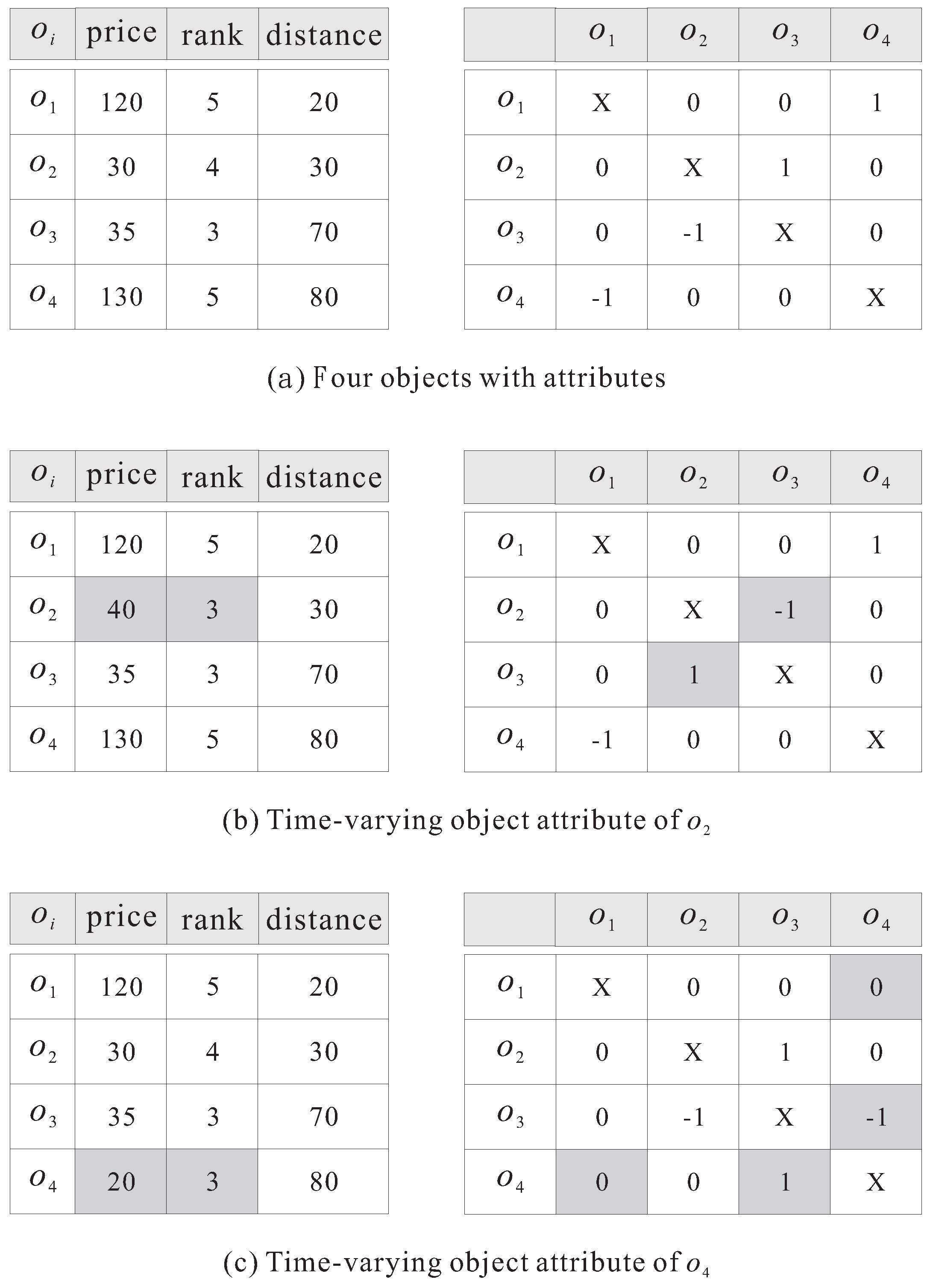
The of node n can be updated by considering that each entry in the row containing the object o changing its attribute from to corresponds to which case mentioned above. The example in Figure 4 is used to illustrate how to update the of node n when the time-varying object attribute of object o is changed. As shown in Figure 4a, there are four objects to with two attributes: “price” and “rank” and the “distance” attribute (where the “distance” attribute refers to the road distance of object n). Based on the object attributes and the “distance” attribute, and are dominated by and , respectively, and thus, and are the WSOs of n (i.e., ). The OADM of n is also shown in Figure 4a. Suppose that object ’s “price” and “rank” attributes are changed from 30 to 40 and from four to three, respectively. Due to the change of ’s attributes, the value of entry in the row and the column containing in the OADM has been updated (refer to Figure 4b). As objects and and in the OADM are changed from one to , meaning that now is dominated by in terms of “price” and “rank” attributes, the is updated according to the fourth condition of the second case. Although, , is still kept in the because of its better “distance” attribute than . As for , it can be added to the as and . That is, . Let us consider another scenario where object changes its “price” (“rank”) attribute from 130 (5) to 20 (3). The time-varying object attribute of affects the dominance relationship between and , as well as and . As shown in Figure 4c, the values of entries and are changed to zero and one, respectively. For the case that , and changing from to zero, which corresponds to the first condition of the third case, is added to the . For the case that , and updating from zero to one, corresponding to the last condition of the fourth case, the is not affected by . Finally, .
4.2. Processing of Time-Varying Edge Length
Different from the time-varying object attribute, which changes only the value of the entry in the OADM, the time-varying edge length may affect the number of objects in the OADM and the RDSL. Specifically, an object could be added to (or removed from) the OADM and the RDSL because of its decreasing (or increasing) distance affected by the time-varying edge length. Moreover, the time-varying edge length may also result in an adjustment in the order of objects in the RDSL. As such, when the time-varying edge length of an edge e is changed, the OADM, the RDSL and the SOET of node n are updated accordingly, which are then used to determine whether the of node n is affected by edge e’s time-varying edge length.
Consider the case that the length of edge e connecting nodes and is changed from to ∞ (i.e., e is temporarily closed). In the SOET of node n, if there is no parent-child relationship between the tree nodes containing and , then changing e’s length from to ∞ cannot affect the OADM, the RDSL and the SOET of node n, as well as its (i.e., the WSOs result remains valid). Otherwise, the subtrees rooted at the tree nodes containing and are affected by e and removed from the SOET. As a result, the road distances between the node n and the objects contained in the subtrees removed need to be updated by traversing the remaining part of the SOET. Suppose that the updated road distance of object o to node n increases from to . Then, the process of updating the is divided into the following three cases: (1) object o does not appear in the RDSL; (2) object o appears in the RDSL, but ; and (3) object o appears in the RDSL and .
- Object o does not appear in the RDSL: this means that the road distance of object o to node n is greater than the distance d. As , object o cannot appear in the RDSL. Therefore, the need not be updated.
- Object o appears in the RDSL, but : if the updated distance of object o exceeds d, then o is directly removed from the OADM and the RDSL of node n (while the remains unchanged). Otherwise (i.e., ), the order of the RDSL has to be adjusted according to . As for the OADM and the obtained by previous, they are still valid because o’s dominance relationship is not affected and .
- Object o appears in the RDSL and : in the case where the updated distance is greater than d, object o needs to be removed from the OADM, the RDSL and the of node n (meaning that the WSOs result has been changed). In addition, some object, say , that appears in the RDSL, but not in the , can be promoted to the skyline object if it is dominated only by object o (i.e., in the OADM and o is in front of in the RDSL). By looking up the row containing o in the previous OADM, we know the objects with . For each object , if there is no object such that in the OADM and is in front of in the RDSL, then can be added to as it is now a skyline object, and its distance to n is within the distance range d. In the case where the updated distance , object o is still kept in the OADM and the RDSL, but it has a higher position in the RDSL than before. In this case, object o could be removed from the because of its increasing . Conversely, the objects previously dominated by o have a chance to be added to the if they are no longer dominated. To determine whether object o is removed from the or not, the row containing o in the OADM is first checked to find each object with , and then, the updated position of o in the RDSL is compared to that of . Object o is removed from the only when is in front of o. On the other hand, to determine whether object previously dominated by object o can be added to the , each object that has in the OADM and is behind o in the RDSL is considered. Once is now in front of o (that is, is no longer dominated by o) and no object in front of and can be found, is added to the . Otherwise, is still dominated by , so that .
Consider the case that the length of edge e connecting nodes and is changed from ∞ to (that is, e is now passable). If nodes and are not contained in the tree nodes of the SOET of node n, which implies that edge e falls outside the distance range d, then the OADM, the RDSL and the obtained previously remain valid regardless of changing e’s length from ∞ to . In other words, the OADM, the RDSLand the may need to be updated if any tree node of the SOET contains or . This is because the road distances between node n and the objects affected by edge e may further decrease, leading to more or less objects in the OADM, the RDSL and the . Therefore, a grown network expansion starting from and is performed to include the objects whose decreasing distances (attributed to e) are less than or equal to d. Furthermore, the subtree rooted at the tree node containing (or ) is updated accordingly to contain information of such objects. Suppose that the road distance of each affected object o to node n decreases from to (note that ). Similar to the case mentioned above, whether the needs to be updated can be determined based on: (1) object o does not appear in the RDSL; (2) object o appears in the RDSL, but ; and (3) object o appears in the RDSL and .
- Object o does not appear in the RDSL: as the updated road distance of object o to node n is less than or equal to d, object o has to be added into the OADM (where the values of entries in the row and the column containing o are computed using Equation (1)) and the RDSL (in which the order of o is determined according to its ), resulting in that (a) object o could be added into the and (b) some object could be removed from the . For (a), if there is an object with in the OADM and in front of o in the RDSL, then o is still dominated by and, thus, cannot be added to the . Otherwise, . For (b), object is removed from the only when o is better than in terms of the object attributes and the “distance” attribute. Therefore, if the entry exists in the OADM and o is in front of in the RDSL, then is removed from .
- Object o appears in the RDSL, but : as , object o has a better order in the RDSL than before. As a result, there is a chance that object behind o’s current position in the RDSL (meaning that o is better than in the “distance” attribute) is now dominated by o. Having checked the row containing o in the OADM, such an object can be removed from the if exists in the OADM (that is, o is also better than in the object attributes). On the other hand, due to the decreasing distance , all of the objects in front of o may no longer dominate o so that o can be added to the . Consider again the row containing o in the OADM. If no entry , where is in front of o in the RDSL, can be found, then o is promoted to a skyline object (i.e., ).
- Object o appears in the RDSL and : in this case, object o would still be kept in the because its road distance decreases to . Furthermore, o may dominate the other objects in the , as it now has a better “distance” attribute. For each object , once the two conditions that in the OADM and o is in front of in the RDSL hold, is removed from the .
4.3. Processing of the Time-Varying Query Path
Given the query path , the continuous within skyline query finds the WSOs for each point on . Moreover, the OADM, the RDSL, the SOET and the of each node n on are maintained for efficient processing of the time-varying information. Nevertheless, the query path may be changed to due to the road congestions or accidents on some roads (i.e., edges) belonging to , making the OADM, the RDSL, the SOET and the of the two nodes connecting such edges outdated.
To process the time-varying query path, each edge e belonging to is first determined because the OADM, the RDSL and the SOET of node n connecting e remain valid, as well as its . Then, it is only necessary to execute the continuous within skyline query for the remaining part of the updated query path (that is, ), so as to obtain the WSOs of the nodes on and also their OADM, RDSL and SOET. The procedure of the within skyline object updating algorithm is detailed in Algorithm 1.
| Algorithm 1: The within skyline object updating algorithm. |
 |
5. Performance Evaluation
In this section, we first conduct two sets of experiments to investigate the efficiency of the proposed within skyline object updating algorithm, compared to the Cd-SQ algorithm in [8] which operates without the support of the OADM, the RDSL and the SOET presented in this paper. The first set of experiments studies the effects of four important factors on the performance of processing the continuous within skyline query. The second one investigates how well the within skyline object updating algorithm and its competitor work for dynamic road networks. Then, we discuss the space requirements of the within skyline object updating algorithm and the Cd-SQ algorithm, respectively.
5.1. Experimental Settings
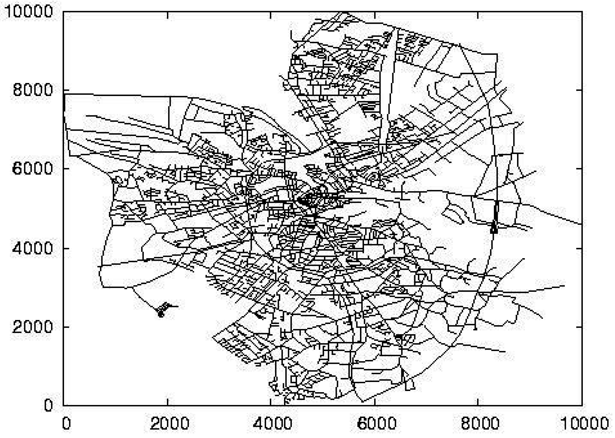
All experiments are performed on a PC with AMD Athlon X2 5200 CPU and 2 GB RAM. The algorithms are implemented in C++. As shown in Figure 5, the road map, Oldenburg (a city in Germany) [23], consisting of about 6000 nodes and 7000 edges, is used in our simulation. The set of data objects (varying from 10 K to 200 K) is generated using the generator proposed in [24], which is the most popular framework used in road networks [25,26,27]. Each data object has several attributes (ranging from two to six) whose values are normalized in the range . In the experimental space, we also generate 30 query paths, each of which consists of multiple edges (ranging from one to 16). For each query path , we perform a continuous within skyline query to find the WSOs for each point on , in which the distance d varies from to of the entire space. Based on the WSOs result obtained, the OADM, the RDSL and the SOET of each node belonging to are maintained for the within skyline object updating algorithm. To investigate the effect of the time-varying information on the performance of the proposed approaches, for each query path , we set the default number of updates to 20, and each update process involves of objects changing their attributes (where x varies from zero to 20), of edges updating their lengths (in which y varies from zero to 16), and of edges on affected by the time-varying query path (where z varies from zero to 25). The performance is measured by the average CPU time in performing workloads of 30 continuous within skyline queries with 20 updates. Table 2 summarizes the parameters under investigation, along with their default values and ranges.
5.2. Effect of Four Important Factors
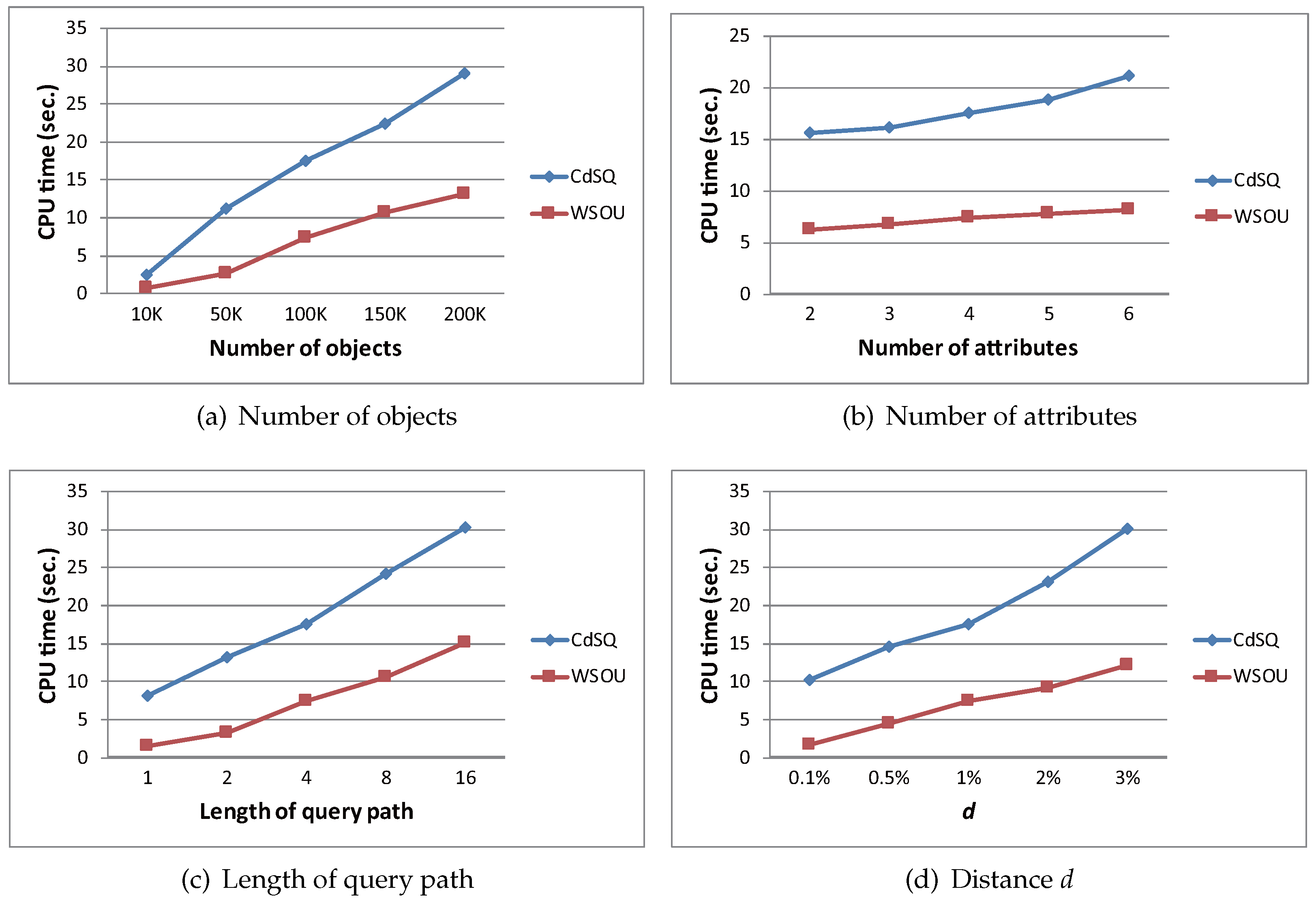
The first set of experiments demonstrates the efficiency of the within skyline object updating algorithm (WSOU) by comparing it with the Cd-SQ algorithm, in terms of the CPU time. Four experiments are implemented to investigate the effects of four important factors on the performance of processing the continuous within skyline query with time-varying information. These important factors are the number of objects, the number of attributes, the length of query path and the value of d.
Figure 6a studies the effect of the number of objects on the performance of the WSOU algorithm and the CdSQ algorithm. In this experiment, we vary the number of objects from 10 K to 200 K and measure the CPU time for the proposed algorithms. As we can see from the simulation, the performance gap between the WSOU algorithm and the CdSQ algorithm increases with the increasing number of objects. The reason is that for the CdSQ algorithm, the query needs to be re-executed whenever an update occurs, so that when the number of objects increases, more processing time is spent on the repetitive query execution. However, for the WSOU algorithm, the query re-execution can be effectively reduced by taking advantage of the three data structures, the OADM, the RDSL and the SOET, because most of the time-varying information actually does not affect the query result and, thus, can be directly ignored.
Figure 6b illustrates the performance of the WSOU algorithm and the CdSQ algorithm as a function of the number of attributes (ranging from two to six). The simulation shows that the performance of the CdSQ algorithm degrades linearly as the number of objects increases, while the WSOU algorithm is not sensitive to the number of attributes. This is because more object attributes would result in more skyline objects (in terms of the object attributes), and thus, more dominance tests are performed for the CdSQ algorithm. The simulation confirms again that applying the OADM, the RDSL and the SOET in the WSOU algorithm can efficiently improve the performance of processing the continuous within skyline query with time-varying information.
In Figure 6c, we investigate the efficiency of the WSOU algorithm and the CdSQ algorithm by measuring the CPU cost under different lengths of query path (varying from one to 16 edges). When the length of query path increases, the CPU overhead for both algorithms increases because for a longer query path, (1) the CdSQ algorithm takes more CPU time to determine the new query result affected by each update and (2) the WSOU algorithm requires building more OADM, RDSL and SOET for the nodes belonging to the query path. Nevertheless, the WSOU algorithm outperforms its competitor in all cases. The improvement is due to the fact that the WSOU algorithm considers only the time-varying information affecting the query result (however, the CdSQ algorithm needs to re-execute the query no matter whether the result is affected or not).
Finally, in Figure 6d, we compare the performance of the WSOU algorithm and the CdSQ algorithm with respect to different values of d (ranging from to ). For the WSOU algorithm, a greater d leads to more objects kept in the OADM, the RDSL and the SOET (i.e., more objects with the distance range d), and thus, the required CPU time increases slightly with the increasing d (but basically, the CPU time is still under 10 s). For the CdSQ algorithm, a smaller d is favorable because less computation of road distances of the objects within the distance range d has to be performed. However, when d increases to a larger value (e.g., ), meaning that more qualifying objects are considered, the CPU cost of the CdSQ algorithm becomes much higher than that of the WSOU algorithm (because it has no chance of avoiding the query re-execution).
5.3. Effect of Time-Varying Information
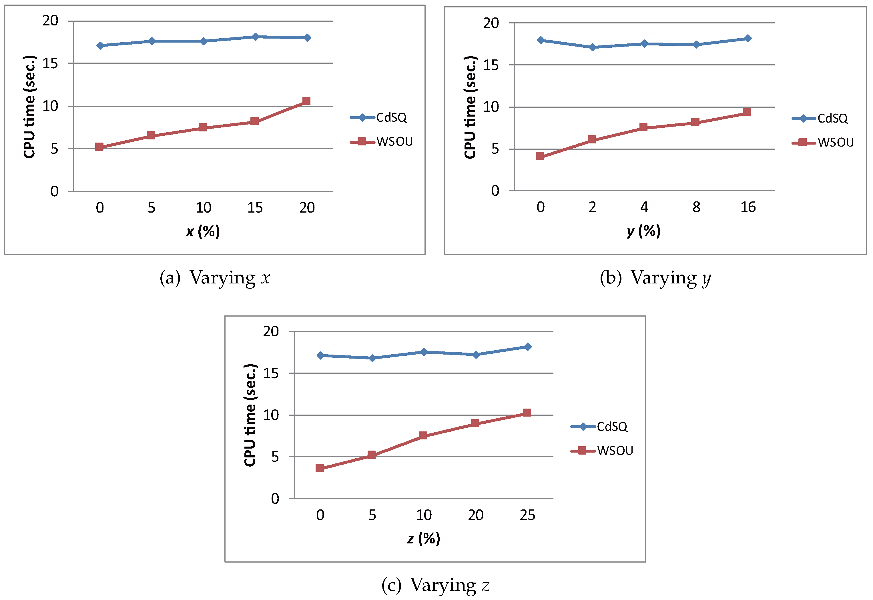
The second set of experiments studies how well the WSOU algorithm and the CdSQ algorithm work for dynamic road networks by varying the percentages of: (1) objects changing attributes; (2) edges updating lengths; and (3) affected edges on the query path. Hereafter, for the x-axis in the figures, the three percentages refer to , and , respectively.
Figure 7a investigates the impact of various numbers of objects changing their attributes (i.e., varying ) on the performance of the WSOU algorithm and the CdSQ algorithm. In the experiment, we vary from to and measure the CPU cost for the two algorithms. The simulation shows that the WSOU algorithm outperforms the CdSQ algorithm by a factor of to three in terms of the CPU time. The large difference in CPU time between the two algorithms comes from: (1) for the CdSQ algorithm, the query re-execution at each update is inevitable, no matter what the number of objects changing attributes is (that is why its cost keeps almost constant); while (2) for the WSOU algorithm, the query re-execution can be avoided by determining which of the objects changing attributes fall outside the distance range d and by only updating the affected query result if necessary, utilizing the OADM, the RDSL and the SOET.
In Figure 7b, we measure the CPU overhead of the WSOU algorithm and the CdSQ algorithm under different numbers of edges changing lengths (ranging from to ). Similar to the reason explained in the previous experiment, the CPU time for the CdSQ algorithm is nearly constant as the number of edges changing lengths increases (i.e., increasing ). As for the WSOU algorithm, its CPU time shows an increasing trend because as y becomes greater, the chance of the edge falling within the distance range d increases so that more distance updates of objects are required. Nevertheless, the WSOU algorithm can still achieve better performance than the CdSQ algorithm in all cases (by a factor of up to two), as the affected object distances can be updated by traversing the SOET (but for the CdSQ algorithm, Dijkstra’s algorithm or the A* algorithm must be executed to compute the affected distances).
The last experiment shown in Figure 7c evaluates the effect of the time-varying query path on the CPU time of the WSOU algorithm and the CdSQ algorithm, in which ranges from to . A large value of z leads to more number of edges belonging to the query path and affected by the time-varying query path (that is, more edges belonging to , where is the updated query path). For the WSOU algorithm, the CPU cost increases with z, because more processing time is required for determining the WSOs of edges belonging to using the continuous within skyline query. Note that the WSOs of edges belonging to are still valid, for which the continuous within skyline query need not be executed. For the CdSQ algorithm, the CPU time is almost not affected by the value of z. The reason is that the continuous within skyline query has to be re-executed, regardless of whether the query path is changed or not. Again, the simulation shows that the WSOU algorithm performs better than the CdSQ algorithm in all cases.
5.4. Discussion of the Space Requirement
In this subsection, we discuss the space complexity of the WSOU algorithm and the CdSQ algorithm, in terms of the data structures used in query processing. For the CdSQ algorithm (refer to [8]), three tables, , and , are used to represent the road network and maintain information of data objects. During the course of query processing, the query path is divided into a set of edges, each of which requires a set to keep the within skyline objects on it. Assume that the query path consists of n edges, and the average size of set for each edge is . The space complexity of the CdSQ algorithm is estimated as , where , and refer the sizes of the tables , and , respectively. For the WSOU algorithm, in addition to the required space of the CdSQ algorithm, the data structures OADM, RDSL and SOET are needed to maintain the information of the dominance relationships and the road distances of objects. For the query path consisting of n edges, there are nodes connecting the edges, and in each node, the three data structures are used to facilitate handling the time-varying information. Let , and be the average sizes of the OADM, the RDSL and the SOET, respectively. Then, the space requirement for the WSOU algorithm is . Although the WSOU algorithm slightly sacrifices the space cost compared to the CdSQ algorithm, it can greatly improve the performance of processing the continuous within skyline query in dynamic road networks, which has been demonstrated in the above simulations.
6. Conclusions
This paper focuses on efficiently processing the continuous within skyline queries in dynamic road networks, where the attributes of objects, the lengths of edges and the query paths may vary with time (called the time-varying information). To provide real-time processing of the continuous within skyline queries with time-varying information, we design three data structures, the OADM, the RDSL and the SOET, to adequately maintain information of objects and road network. Based on the three data structure, we further develop the within skyline object updating algorithm to quickly determine whether the query result is affected by the time-varying information and rapidly update the new result if necessary. Extensive experiments have been conducted to demonstrate the efficiency of the proposed approaches.
There are several interesting avenues for the future extensions of this work. One important avenue is to cope with other variations of the skyline queries, such as the continuous k nearest neighbor queries [8], in dynamic road networks with time-varying information. Another extension is to extend the within skyline object updating algorithm to be suitable for the highly dynamic environment, in which all objects move as time passes (implying that the object locations change with time). An important extension is to study the possibility of applying the within skyline object updating algorithm to distributed environments, such as the sensor networks [28,29,30].
Acknowledgments
This work was supported by the Ministry of Science and Technology of Taiwan under Grant MOST 105-2119-M-022-002 and Grant MOST 104-2119-M-022-001.
Conflicts of Interest
The author declares no conflict of interest.
References
- Benetis, R.; Jensen, C.S.; Karciauskas, G.; Saltenis, S. Nearest Neighbor and Reverse Nearest Neighbor Queries for Moving Objects. VLDB J. 2006, 15, 229–249. [Google Scholar] [CrossRef]
- Huang, Y.K.; Kuo, W.H.; Lee, C.; Wang, T.H. Shortest Average-Distance Query on Heterogeneous Neighboring Objects. In Proceedings of the International Conference on IDEAS, Yokohoma, Japan, 13–15 July 2015; pp. 116–125. [Google Scholar]
- Mokbel, M.F.; Xiong, X.; Aref, W.G. SINA: Scalable Incremental Processing of Continuous Queries in Spatio-temporal Databases. In Proceedings of the ACM SIGMOD, Paris, France, 13–18 June 2004; pp. 623–634. [Google Scholar]
- Tao, Y.; Papadias, D. Time-parameterized queries in spatio-temporal databases. In Proceedings of the ACM SIGMOD, Madison, WI, USA, 2–6 June 2002; pp. 334–345. [Google Scholar]
- Borzsonyi, S.; Kossmann, D.; Stocker, K. The skyline operator. In Proceedings of the 17th International Conference on Data Engineering, Heidelberg, Germany, 2–6 April 2001; pp. 421–430. [Google Scholar]
- Huang, Z.; Lu, H.; Ooi, B.C.; Tung, A. Continuous Skyline Queries for Moving Objects. IEEE Trans. Knowl. Data Eng. 2006, 18, 1645–1658. [Google Scholar] [CrossRef]
- Sharifzadeh, M.; Shahabi, C. The Spatial Skyline Queries. In Proceedings of the International Conference on Very Large Data Bases, Seoul, Korea, 12–15 September 2006; pp. 751–762. [Google Scholar]
- Huang, Y.K.; Chang, C.H.; Lee, C. Continuous distance-based skyline queries in road networks. Inf. Syst. 2012, 37, 611–633. [Google Scholar] [CrossRef]
- Bentley, J.L.; Kung, H.T.; Schkolnick, M.; Thompson, C.D. On the average number of maxima in a set of vectors and applications. J. ACM 1978, 25, 536–543. [Google Scholar] [CrossRef]
- Chomicki, J.; Ciaccia, P.; Meneghetti, N. Skyline Queries, Front and Back. ACM SIGMOD Rec. 2013, 42, 6–18. [Google Scholar] [CrossRef]
- Hsueh, Y.L.; Hascoet, T. Caching Support for Skyline Query Processing with Partially Ordered Domains. IEEE Trans. Knowl. Data Eng. 2014, 26, 2649–2661. [Google Scholar] [CrossRef]
- Kung, H.T.; Luccio, F.; Preparata, F.P. On finding the maxima of a set of vectors. J. ACM 1975, 22, 469–476. [Google Scholar] [CrossRef]
- Mortensen, M.L.; Chester, S.; Assent, I.; Magnani, M. Efficient caching for constrained skyline queries. In Proceedings of the International Conference on Extending Database Technology, Brussels, Belgium, 23–27 March 2015. [Google Scholar]
- Cheema, M.A.; Lin, X.; Zhang, W.; Zhang, Y. A Safe Zone Based Approach for Monitoring Moving Skyline Queries. In Proceedings of the International Conference on Extending Database Technology, Genoa, Italy, 18–22 March 2013. [Google Scholar]
- Zheng, J.; Chen, J.; Wang, H. Efficient Geometric Pruning Strategies for Continuous Skyline Queries. ISPRS Int. J. Geo-Inf. 2017, 6, 91. [Google Scholar] [CrossRef]
- Vu, K.; Zheng, R. Efficient Algorithms for Spatial Skyline Query With Uncertainty. In Proceedings of the 21st ACM SIGSPATIAL International Conference on Advances in Geographic Information Systems (ACM SIGSPATIAL), Orlando, FL, USA, 5–8 November 2013. [Google Scholar]
- Deng, K.; Zhou, X.; Shen, H.T. Multi-source skyline query processing in road networks. In Proceedings of the 23rd International Conference on Data Engineering, Istanbul, Turkey, 11–15 April 2007; pp. 796–805. [Google Scholar]
- Zou, L.; Chen, L.; Ozsu, M.T.; Zhao, D. Dynamic Skyline Queries in Large Graphs. In Proceedings of the International Conference on Database Systems for Advanced Applications, Tsukuba, Japan, 1–4 April 2010. [Google Scholar]
- Kriegel, H.P.; Renz, M.; Schubert, M. Route Skyline Queries: A Multi-Preference Path Planning Approach. In Proceedings of the International Conference on Data Engineering, Long Beach, CA, USA, 1–6 March 2010. [Google Scholar]
- Mouratidis, K.; Lin, Y.; Yiu, M.L. Preference Queries in Large Multi-Cost Transportation Networks. In Proceedings of the International Conference on Data Engineering, Long Beach, CA, USA, 1–6 March 2010. [Google Scholar]
- Huang, X.; Jensen, C.S. In-Route Skyline Querying for Location-based Services. In Proceedings of the International Workshop on Web and Wireless Geographical Information Systems, Goyang, Korea, 26–27 November 2004; pp. 120–135. [Google Scholar]
- Jang, S.M.; Yoo, J.S. Processing Continuous Skyline Queries in Road Networks. In Proceedings of the International Symposium on Computer Science and its Applications, Hobart, Australia, 13–15 October 2008. [Google Scholar]
- TIGER. Available online: http://www.census.gov/geo/www/tiger/ (accessed on 28 April 2017).
- Brinkhoff, T. A Framework for Generating Network-Based Moving Objects. GeoInformatica 2002, 6, 153–180. [Google Scholar] [CrossRef]
- Cheema, M.A.; Zhang, W.; Lin, X.; Zhang, Y.; Li, X. Continuous reverse k nearest neighbors queries in Euclidean space and in spatial networks. VLDB J. 2012, 21, 69–95. [Google Scholar] [CrossRef]
- Guting, R.H.; de Almeida, V.T.; Ding, Z. Modeling and querying moving objects in networks. VLDB J. 2006, 15, 165–190. [Google Scholar] [CrossRef]
- Mouratidis, K.; Yiu, M.L.; Papadias, D.; Mamoulis, N. Continuous Nearest Neighbor Monitoring in Road Networks. In Proceedings of the International Conference on VLDB, Seoul, Korea, 12–15 September 2006. [Google Scholar]
- Buonanno, A.; D’Urso, M.; Prisco, G.; Felaco, M.; Meliado, E.F.; Mattei, M.; Palmieri, F.; Ciuonzo, D. Mobile Sensor Networks based on Autonomous Platforms for Homeland Security. In Proceedings of the Tyrrhenian Workshop on Advances in Radar and Remote Sensing, Naples, Italy, 12–14 September 2012. [Google Scholar]
- Ciuonzo, D.; Buonanno, A.; D’Urso, M.; Palmieri, F.A. Distributed Classification of Multiple Moving Targets with Binary Wireless Sensor Networks. In Proceedings of the International Conference on Information Fusion, Chicago, IL, USA, 5–8 July 2011. [Google Scholar]
- Tsiligkaridis, T.; Sadler, B.M.; Hero, A.O. On Decentralized Estimation with Active Queries. IEEE Trans. Signal Process. 2015, 63, 2610–2622. [Google Scholar] [CrossRef]
Figure 1.
Example of the continuous within skyline query.

Figure 2.
Three data structures: object attribute dominating matrix (OADM), the road distance sorted list (RDSL) and the skyline object expansion tree (SOET).
Figure 2.
Three data structures: object attribute dominating matrix (OADM), the road distance sorted list (RDSL) and the skyline object expansion tree (SOET).

Figure 3.
Update of the SOET.

Figure 4.
Example of processing the time-varying object attribute.

Figure 5.
Oldenburg road network.

Figure 6.
Effect of four important factors. WSOU, within skyline object updating.

Figure 7.
Effect of time-varying information.


Table 1.
The notations.
| Notation | Description |
|---|---|
| a set of data objects | |
| a path along which the query object moves | |
| d | a user-defined distance |
| WSOs | the within skyline objects |
| Time-varying object attribute | o changes its attribute from to |
| Time-varying edge length | e’s length is changed from to ∞ or from ∞ to |
| Time-varying query path | is changed to |
Table 2.
System parameters.
| Parameter | Default | Range |
|---|---|---|
| Number of objects | 100 (K) | 10, 50, 100, 150, 200 (K) |
| Number of attributes | 4 | 2, 3, 4, 5, 6 |
| Length of path length | 4 | 1, 2, 4, 8, 16 |
| Distance d | 0.1, 0.5, 1, 2, 3 | |
| Time-varying object attribute x | 0, 5, 10, 15, 20 | |
| Time-varying edge length y | 0, 2, 4, 8, 16 | |
| Time-varying query path z | 0, 5, 10, 20, 25 |
© 2017 by the author. Licensee MDPI, Basel, Switzerland. This article is an open access article distributed under the terms and conditions of the Creative Commons Attribution (CC BY) license (http://creativecommons.org/licenses/by/4.0/).
Share and Cite
MDPI and ACS Style
Huang, Y.-K. Within Skyline Query Processing in Dynamic Road Networks. ISPRS Int. J. Geo-Inf. 2017, 6, 137. https://doi.org/10.3390/ijgi6050137
AMA Style
Huang Y-K. Within Skyline Query Processing in Dynamic Road Networks. ISPRS International Journal of Geo-Information. 2017; 6(5):137. https://doi.org/10.3390/ijgi6050137
Chicago/Turabian StyleHuang, Yuan-Ko. 2017. "Within Skyline Query Processing in Dynamic Road Networks" ISPRS International Journal of Geo-Information 6, no. 5: 137. https://doi.org/10.3390/ijgi6050137
Note that from the first issue of 2016, this journal uses article numbers instead of page numbers. See further details here.