Article

Determination of 3D Displacements of Drainage Networks Extracted from Digital Elevation Models (DEMs) Using Linear-Based Methods

by
Antonio Tomás Mozas-Calvache
*,
Manuel Antonio Ureña-Cámara
and
Francisco Javier Ariza-López
Department of Cartographic, Geodetic Engineering and Photogrammetry, University of Jaén, 23071 Jaén, Spain
*
Author to whom correspondence should be addressed.
ISPRS Int. J. Geo-Inf. 2017, 6(8), 234; https://doi.org/10.3390/ijgi6080234
Submission received: 15 June 2017 / Revised: 14 July 2017 / Accepted: 2 August 2017 / Published: 4 August 2017

Abstract

:
This study describes a new method developed to determine the 3D positional displacements of the drainage networks extracted from Digital Elevation Models (DEMs). The proposed method establishes several stages for data preparation. The displacements are derived by means of linestring-based assessment methods, which can be applied in 2D and 3D. Also, we propose the use of several tools (maps, aggregation of results, new indices, etc.) in order to obtain a wider assessment of positional accuracy, or a time change analysis. This approach supposes a novelty in drainage network studies both in the application of line-based methods and its expansion to 3D data. The method has been tested using a sample of channels extracted from DEMs of two different dates of a zone of about 600 square kilometers using as reference linestrings those extracted from another more recent DEM which had higher spatial accuracy and higher spatial resolution. The results have demonstrated the viability of the method proposed because of the obtaining of 3D displacement vectors, which showed the general and particular behavior of the channels selected.

1. Introduction

The current availability of cartographic products related to height data such as Digital Elevation Models (DEMs) is achieving global coverage thanks to the launch of new acquisition systems such as those based on remote sensing. As an example, the ASTER GDEM (Advanced Spaceborne Thermal Emission and Reflection Radiometer Global Digital Elevation Model) coverage spans from a latitude of 83 degrees north to 83 degrees south [1] with 30 m of spatial resolution. Additionally, the development of photogrammetric techniques and Light Detection and Ranging (LiDAR) and their application using Unmanned Aerial Systems (UAS) allow the obtaining of DEMs with higher spatial resolutions and lower cost to producers. Furthermore, the development of Spatial Data Infrastructures (SDIs) allows users access to height data products shared on the Internet by cartographic institutions and enterprises with certain levels of updating. All these aspects are causing a great availability of these digital products from several sources and dates, which allow the implementation of comparative studies of DEMs and other derived products. As an example, the implementation of multi-temporal studies to analyze the evolution of the Earth’s surface, and more specifically of drainage networks.
A drainage network includes all the stream channels that drain toward a reference point [2]. Drainage channels are the lines along which fluvial processes act to transport water and mineral material out of a local region, allowing gravity processes on slopes to continue to lower landscapes [3]. In this context, one of the main features extracted from height data, and more specifically from regular-grid DEMs, has been drainage networks. The extraction of drainage networks from digital elevation data is important for qualitative studies in geomorphology and hydrology [3]. Several studies have described algorithms for extracting drainage networks from regular-grid DEMs [3,4,5,6,7,8,9,10]. As a consequence of the application of these algorithms, a set of lines (or linestrings) which represents the drainage channels is obtained.
The assessment of the positional accuracy of DEMs has been based mainly on the comparison of the positions of a sample of well-defined points to their positions regarding a more accurate source. This assessment is usually based on the determination of the Root Squared Mean Error (RMSE) of the differences of their coordinates. In this context, several standards [11,12,13] and approaches [14,15,16,17,18,19] have been described and applied until this time. These methods have been extended to assessing the positional accuracy of drainage networks obtained from aerial photogrammetry [20], LiDAR data [21] and remote sensing [22]. However, it is possible to use other elements instead of points in order to assess the accuracy of DEMs, and more specifically of the extracted drainage networks. In this context, Reinoso [23] estimated the horizontal displacements by calculating the area within homologous contours present in two different DEMs, Mozas et al. [24] used axes extracted from the boundaries of the river channels digitized from orthoimages to analyze planimetric changes, and Mozas et al. [25] analyzed the positional accuracy of several sets of contour lines obtained from a DEM. In summary, drainage networks are mainly characterized by the lines which represent the channels. Thus, it seems logical that studies which compare these elements may be carried out using linear-based methods.
The positional assessment of lines was initially based on the concept of the uncertainty band or Epsilon Band described by Perkal [26]. This band contained the more probable location of the line. Since then, various models [27,28,29,30,31,32,33] and methods [34,35,36,37,38,39,40] have been proposed for describing and assessing the positional accuracy of lines. A more detailed description of these models and methods was outlined by Gil de la Vega et al. [41]. As an example, some elements assessed using these linear-based methods were coastlines [37], roads and/or railways [36,38,42], river channels [24] and contour lines [25]. However, the majority of these studies analyzed the positional displacements of a set of lines from a planimetric point of view. In this sense, Mozas and Ariza [40] adapted several methods to assess and control lines in 3D using a more accurate source of lines. Among others, they adapted to 3D the Hausdorff distance method (HDM) and the Vertex Influence Method (VIM3D). The first is based on the determination of the maximum distance between lines (Hausdorff Distance) and was initially used in 2D by Abbas et al. [36]. The VIM3D method consisted of the determination of the 3D displacement vectors between the vertexes of the control line (reference line) with respect to the line to be controlled (assessed). The average 3D displacement vector of the line was calculated by weighting each vector by the length of the segments adjacent to each vertex [40].
To summarize, in this study a new methodology is proposed in order to determine displacements of drainage networks, and more specifically drainage channels, using 3D positional assessment methods based on lines. This contribution allows us to determine maximum and mean displacements of drainage channels in 2D, 3D, globally and particularly. The main goal is to detect and quantify significant positional changes between drainage channels from several sources or dates both in a general and particular way (networks and channels). As an example, some of the possible applications are the determination of the changes of drainage channels obtained from several sources, including the positional assessment of them (using as control or reference dataset a more accurate source), the study of the evolution of drainage networks using multi-temporal datasets of lines, etc. To test this methodology, we have used two datasets of lines which correspond to drainage channels extracted from two DEMs produced and shared on the Internet by an environmental institution in Spain and dated in 1977 and 2010. We used as reference dataset the lines extracted from a more recent and accurate DEM of the same zone with higher spatial resolution.

2. Methodology

The methodology proposed in this study is summarized in Figure 1. Note that during the rest of the paper, we will use channels or linestrings interchangeably. Both represent the same feature but the first in a hydrological way and the last in a geometrical way. Moreover, we will exchange control linestrings as the reference channels and assessed linestrings as the channels for which displacements should be determined. The process is divided into four stages which correspond to: (1) the obtaining of the datasets of linestrings to be assessed and to be used as control elements (reference), (2) the selection and preparation of the linestrings, (3) the application of the positional assessment methods based on lines, and (4) the final analysis of the results. Each stage is detailed further in the following sections.

2.1. Obtaining of the Datasets to Be Used

As mentioned previously, the main goal of this study is to determine displacements of drainage networks extracted from DEMs using linear-based methods. Thus, the drainage channels which compose the drainage networks to be assessed are extracted from a DEM obtaining a set of linestrings (LIN1 in Figure 1). This extraction can be performed using any of the algorithms outlined up to this moment and implemented in some software applications [3,4,5,6,7,8,9,10]. To assess this dataset, we use another set of linestrings obtained from a more accurate source (CTR1 in Figure 1). In this context, there is the possibility of obtaining this reference dataset (CTR1) by extracting channels from another reference DEM (option 1 in Figure 1) or directly from a vector source (e.g., an official cartographic source) (option 2 in Figure 1). In both cases, the positional accuracy of the source must guarantee a certain level of accuracy in order to be used as reference dataset. In this sense, we propose using a point-based method in order to obtain the relative level of accuracy between both sources (LIN1 and CTR1). For a general case, the methodology proposed in this study includes the assessment of lines in 3D. This supposes that the channels must contain height information. In the case of sources of DEMs (Source 1 and Source 2: Option 1 in Figure 1), the extraction process must be followed by the obtaining of the height of each vertex which composes linestrings. The height is obtained by a bilinear interpolation of each vertex on the original DEM. In the case of using a 2D vector source as reference database (Option 2 in Figure 1), the obtaining of height values can also be based on a bilinear interpolation using an auxiliary more accurate reference DEM. In summary, this first stage includes those procedures needed for obtaining those datasets of linestrings which correspond to the drainage channels to be assessed (LIN1) and to assess (CTR1). Additionally, an official vector source (VCT), which includes information about the channels to be selected (e.g., the channel order), can also be used as mask. As an example, in Europe there is a structured hydrological feature coding system called Catchment Characterization and Monitoring (CCM) [43] which can be used for selecting the channels.

2.2. Selection and Preparation of the Linestrings

The second stage is composed of those procedures needed to select and prepare both datasets in order to implement the positional assessment. It is divided into 3 sub-stages which are described throughout this section: (1) Selection of linestrings, (2) Edition to assure compatibility and (3) Matching of linestrings:
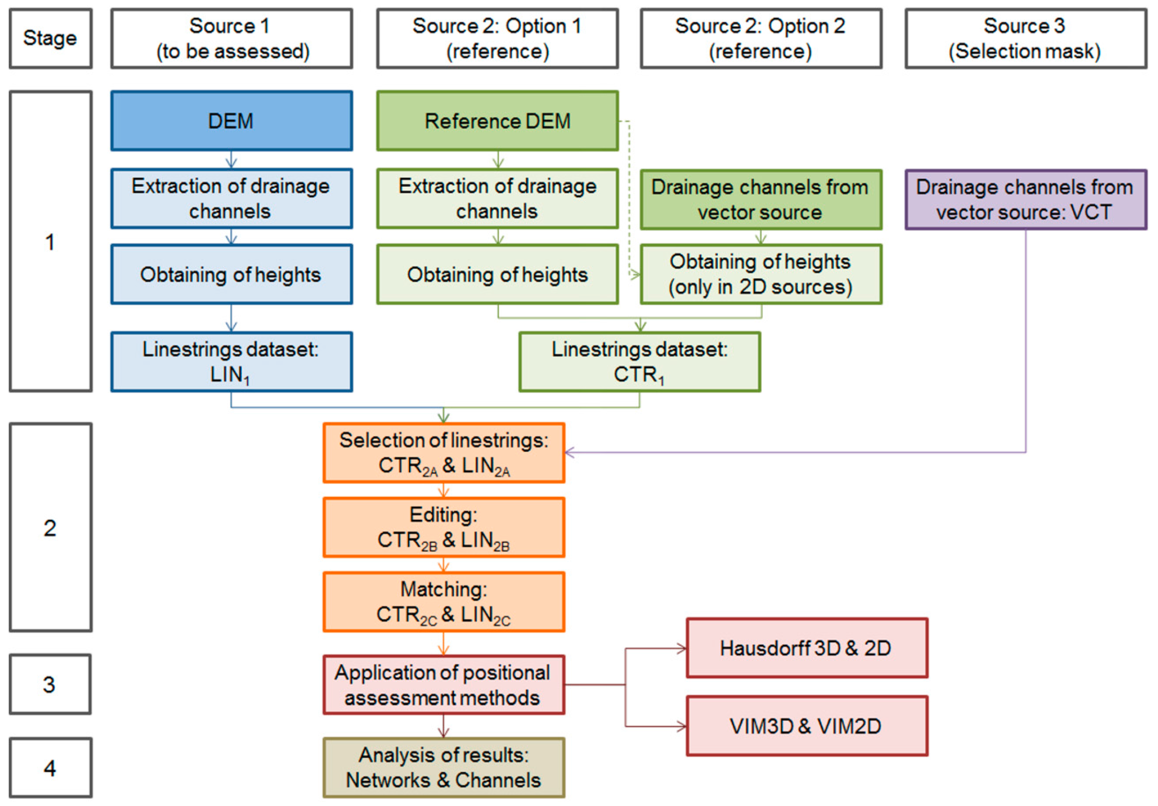
  • Selection of linestrings: The drainage networks extracted from DEMs can be composed of a great quantity of channels. Therefore, a process for selecting elements is needed in order to establish the linestrings of both datasets to be used. Obviously this selection of elements will depend on the purpose of the study to be performed, but in general we consider that this process will initially be based on the availability of elements in the CTR1. In this sense, the origin of the CTR1 dataset plays a great importance in the selection of the linestrings to be used:
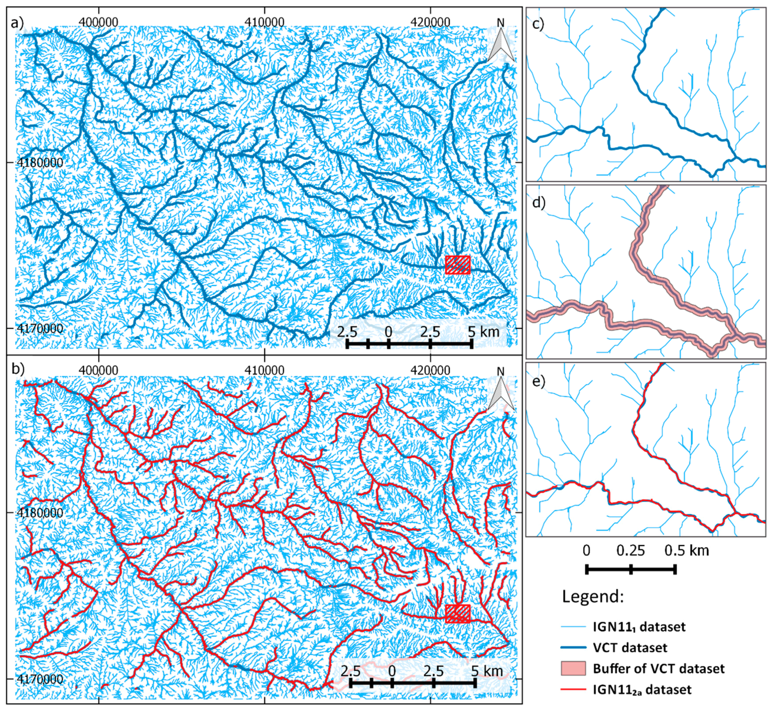
    • DEM source (Option 1): In this case we must consider that the density of the drainage network obtained depends on the threshold of the accumulated area used (e.g., cells with more than 50 cells flowing into them). As the threshold value is increased, the density of the drainage network decreases [5]. A more detailed analysis of this aspect was provided by Tarboton et al. [6] and Chen et al. [44]. Alternatively to the use of this threshold, it is possible to use an auxiliary vector source (VCT in Figure 1) as selection mask by the automatic selection of the CTR1 linestrings which are included in a proximity area (defined by a buffer) which encloses the auxiliary VCT linestrings.
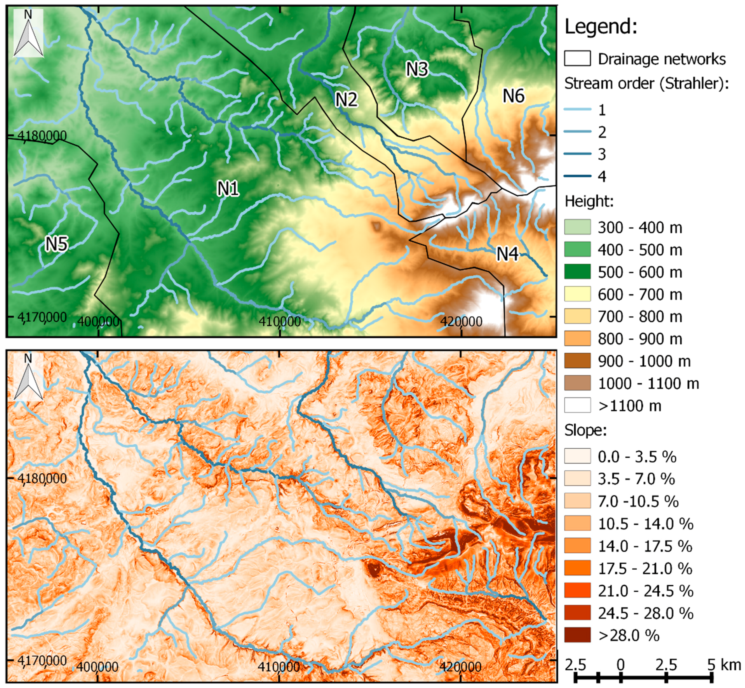
    • Vector source (Option 2): In this case we must consider the scale of the cartographic source and the goal of the study in order to determine the linestrings to be selected. Some attributes included in the vector source can be used to determine the level of importance of the drainage channels to be selected, such as the channel order. As an example, this order can be obtained using the Strahler [45] algorithm. In a similar way to the case of Option 1, another auxiliary vector source (VCT in Figure 1) can also be used as selecting mask.
    A set of linestrings of CTR2A is selected in order to establish the sample of channels to be analyzed. The selection process also includes the determination of the linestrings of the dataset to be assessed (LIN1) which are related to those selected reference linestrings (CTR2A). Here there are several manual or automatic possibilities. We suggest an automatic solution based on the generation of a buffer around the CTR2A linestrings and the spatial intersection of the LIN1 linestrings included in this proximity area. The selection of the width of the buffer must consider the spatial resolution of the DEM and the characteristics of the drainage networks to be studied. We must avoid removing those sections of channels where there are spatial changes greater than this width. Thus, a previous visual analysis of all datasets is recommended in order to determine this width. As a result of this selection, we obtain a dataset to be assessed (LIN2A) and a reference dataset (CTR2A) where there are relationships of proximity between the linestring included in both of them.
  • After the selection of data, an editing is carried out in order to prepare both datasets for an automatic assessment. In this editing process, the linestrings are joined, trimmed or deleted in order to obtain two sets of linestrings which have a certain level of spatial and topological coherence. As an example, two linestrings of LIN2A which correspond to one of CTR2A are joined. The edition stage generates LIN2B and CTR2B datasets.
  • Finally, a matching process is performed in order to establish a unique relationship of each linestring of the LIN2B dataset to one linestring of the CTR2B dataset. The definitive datasets of linestrings are called LIN2C and CTR2C in Figure 1. Both processes of editing and matching can be implemented manually or automatically, as an example using those algorithms described by Mozas and Ariza [42] and Xavier et al. [46].

2.3. Application of the Positional Assessment Methods

The main stage of this methodology consists of the application of positional assessment based on lines to the definitive dataset (LIN2C). As mentioned previously, there are several methods proposed until this moment for this purpose. Some of them have been adapted to 3D by Mozas and Ariza [40]. Taking into account the advantages and disadvantages described by Mozas and Ariza [40], we chose to use the Hausdorff distance method in 3D (HDM3D) in order to obtain maximum values of displacement of each line and the VIM3D method for obtaining the 3D mean displacement vector of each line. Among other advantages of using these methods, we can highlight their easy implementation in 3D with respect to those based on buffers, the obtaining of maximum (HDM3D) and mean values (VIM3D) in order to characterize the displacements and the determination of displacement vectors which are very useful in determining the directions of the displacement. Moreover, using these methods we can determine the distribution functions of displacements of each dataset in the same way as those provided by buffers methods.
Once these methods have been applied for each linestring, we can obtain mean values of the whole dataset or grouped by determined criteria. In addition, depending on the purpose of the study, it could be interesting to divide this assessment into 3D and 2D (using HDM3D, HDM2D, VIM3D and VIM2D) in order to analyze the height behavior independently.

2.4. Analysis of the Results

The final stage consists of the analysis of the results obtained in the previous assessment and the comparison of all the values calculated. The results of the line-based assessment methods are focused on maximum and mean values of displacements and can be grouped in order to analyze complete or partial drainage networks, or particular channels. We propose analyzing these results as a general result but also in relation to slope, stream order and by drainage sub-network. Additionally, other information like the relative positional accuracy between the data sources (e.g., the RMSE of DEMs obtained by the comparison of a sample of points) can be used in order to establish the differences which are given by these sources (e.g., using Federal Geographic Data Committee (FGDC) [11]). We propose the use of a map representing a categorization of the Hausdorff distance (HDM) of each channel in order to perform a visual analysis of areas or channels with larger displacements. We also propose the use of a map representing the mean vector displacement (VIM) of each channel in order to perform a visual analysis of the direction of the displacements. The results can be used to generate some quality indices.

3. Application

An application to a real case was carried out in order to test this methodology. We selected a zone of about 30 × 20 km which corresponds to sheet number 946 of the National Topographic Map of Spain (MTN) (see distribution of MTN sheets in IGN [47]). The selection of this zone was based on the topographical characteristics (heights between 250 and 1500 m with great variability of slopes 0–65%) and the existence of several drainage networks (Figure 2).
The drainage networks to be assessed were extracted from two DEMs (called DEMRED77 and DEMRED10) selected from a temporal series (1977–2010) published on the Internet by the Red de Información Ambiental de Andalucía (Andalusian Environmental Information Network) [48]. The main goal of using two DEMs was to test the ability of the proposed method to detect changes between two datasets of linestrings from two dates or sources.
The reference dataset was extracted from another DEM (called DEMIGN11) of higher spatial resolution and accuracy published by the Instituto Geográfico Nacional (National Geographic Institute of Spain) [47]. Table 1 summarizes the main characteristics of these products. We also used an official vector source (called VCT) published by the Instituto de Estadística y Cartografía de Andalucía (Institute of Statistics and Cartography of Andalusia) [49] which included the drainage channels at scale 1:10,000. This vector source was only used for selecting the channels to be used in this study. Additionally, we obtained the stream order of the drainage networks by applying the Strahler [45] algorithm to VCT (Figure 2). We also considered 6 drainage networks covering the zone of study (Figure 2) which are classified in descending order, taking into account the length of the channels (N1 to N6). Additionally to these data sources, we also used two orthoimages obtained from the same sources of DEMRED77 and DEMRED10 in order to check the results visually.
After selecting these sources of data, the extraction of drainage channels was carried out using ArcGISTM v10.2 software by ESRI® [50] which implements the D8 algorithm [3] following an approach presented by Jenson and Domingue [5]. This process included the determination of the flow directions, the filling of sinks and the delineation of the channels based on the flow accumulation. Following Tarboton et al. [6], two thresholds of 200 cells for 5 m of resolution and 100 cells for 10 of resolution were used in order to determine a large enough amount of drainage channels. As a result of this stage, we obtained two datasets of linestrings which represent the drainage channels to be assessed (RED771-RED101) (LIN1 in Figure 1) and one reference dataset of linestrings (IGN111) (CTR1 in Figure 1). As an example, the IGN111 dataset was initially composed of about 4975 km after the extraction process (Figure 3). The channels selected from the vector source used (VCT) were composed of about 450 km (Figure 3a or Figure 3c) and the definitive IGN112A dataset was composed of about 416 km (Figure 3b or Figure 3e). A buffer of 21 and 42 m semi-width was used depending on the spatial resolution of DEMs (5 and 10 m, respectively) to obtain each dataset. To determine this semi-width value, we considered the diagonal length of cells of each DEM multiplied by 3 (simulating a 3 sigma value). Figure 3d shows an example of the buffer applied to the VCT of 21 m of semi-width to select the linestrings of the IGN111 dataset.
After this stage, all linestrings to be assessed (RED772A-RED102A) and the reference linestrings (IGN112A) were edited and matched in order to obtain datasets of homologous linestrings with a unique correspondence between one linestring of RED772C-RED102C to one linestring of IGN112C. The definitive datasets were composed of more than 300 km in both cases. The next stage consisted of the application of the HDM and the VIM3D method in order to determine the positional differences between the reference dataset (IGN112C) and each dataset to be assessed (RED772C-RED102C). We have to note that, following the suggestions given by Mozas and Ariza [40], we calculated the displacements from the vertexes of the reference linestring with respect to the linestring to be assessed. These calculations were implemented automatically using an application developed in JavaTM for this purpose.

4. Results and Discussion

The main results obtained from the application of the positional assessment methods based on lines to all datasets are summarized in Table 2.
More specifically, Table 2 displays the mean results of the HDM and of the VIM method both in 2D and 3D, and for each coordinate (X, Y, Z). The mean values of maximum displacements (HDM2D) showed differences close to the resolution of the original DEM in both cases. The results of this method in 3D (HDM3D) showed quite similar values to those obtained in 2D. Thus, the contribution of height differences in these results was in the order of centimeters. On the other hand, the mean displacements (VIM2D) showed values lower than the resolution of the DEMs. The mean values of the increments of coordinates obtained using the VIM3D method, which defines a mean displacement vector (dX, dY, dZ in Table 2), showed that the results of dX and dY were closer to zero. The results of dZ also showed lower positive values. This result supposes a mean reduction of heights. To summarize, the results of the displacements estimated using lines showed quite similar behaviors to those estimated using points (relative positional accuracies of DEMs in Table 1). Obviously the values obtained using linestrings were lower than those obtained using points. This is due to the spatial characteristic of lines which can hide those displacements when they are produced in the same direction of lines, as was described in Mozas and Ariza [51]. Table 2 includes the results of Welch’s t-test for population means, weighted by length, for the case of unequal sample sizes and unequal variances. The large p-values obtained in the statistical comparison indicate that, except for the dZ case, there is no significant statistical difference between the RED77 and RED10 datasets. This result will be confirmed below.
Following the analysis developed by Ariza et al. [52], Figure 4 shows the distribution functions by line of the general results obtained in this study. Obviously, all functions show percentages of inclusion (Y-axes in Figure 4) increasing with the displacement (X-axes in Figure 4). Figure 4a,b show the results obtained using HDM while Figure 4c,d show those obtained using VIM. Blue curves show RED77 results and red curves show RED10 results. The HDM cases show higher displacements than the VIM cases at a certain percentage. This is logical considering that HDM values are related to maximum displacements and VIM to mean displacements. The comparison between 2D and 3D results (Figure 4a vs. Figure 4b and Figure 4c vs. Figure 4d) show similar functions although 2D functions show a little better behavior. These results confirm those shown in Table 2 where the 3D displacements have similar values to 2D displacements. The comparison between functions of RED77 and RED10 shows (in general) a better behavior of curves of RED10 with respect to RED77, both in 2D and 3D and using both HDM and VIM methods.
Taking into account that the 2D and 3D results are quite similar because height displacements are considerately lower than planimetric displacements, all the following results in this paper will be shown only for 3D cases.
All these mean results were confirmed using a more detailed visual analysis derived through the graphical representation of the Hausdorff distance and the displacement vectors of each linestring obtained using the VIM3D method (Figure 5 and Figure 6). More specifically, Figure 5 shows the results of Hausdorff distance (HDM3D) by linestring, categorized in three intervals considering the relative positional accuracy of the sources (0–1 s; 1–3 s; >3 s). In general, both figures show values distributed uniformly among these three categories, although the greatest values are mainly concentrated in the flattest zones. An overlap analysis of the categories of these pairs of maps can be used easily to detect large displacement changes between channels of both data sets. Figure 6 shows mean displacement vectors with great variability in directions (see distribution of vectors in Figure 6) and homogeneous distributions in the area both in the XY and Z components. A difference analysis of vectors of homologous elements of these pairs of maps can be used to detect changes in the direction of the displacements of channels of both datasets.
An additional analysis derived from the HDM3D and VIM3D displacements is shown in Figure 7 where these values were distributed taking into account the slope of each segment, the stream order and the drainage network of each linestring:
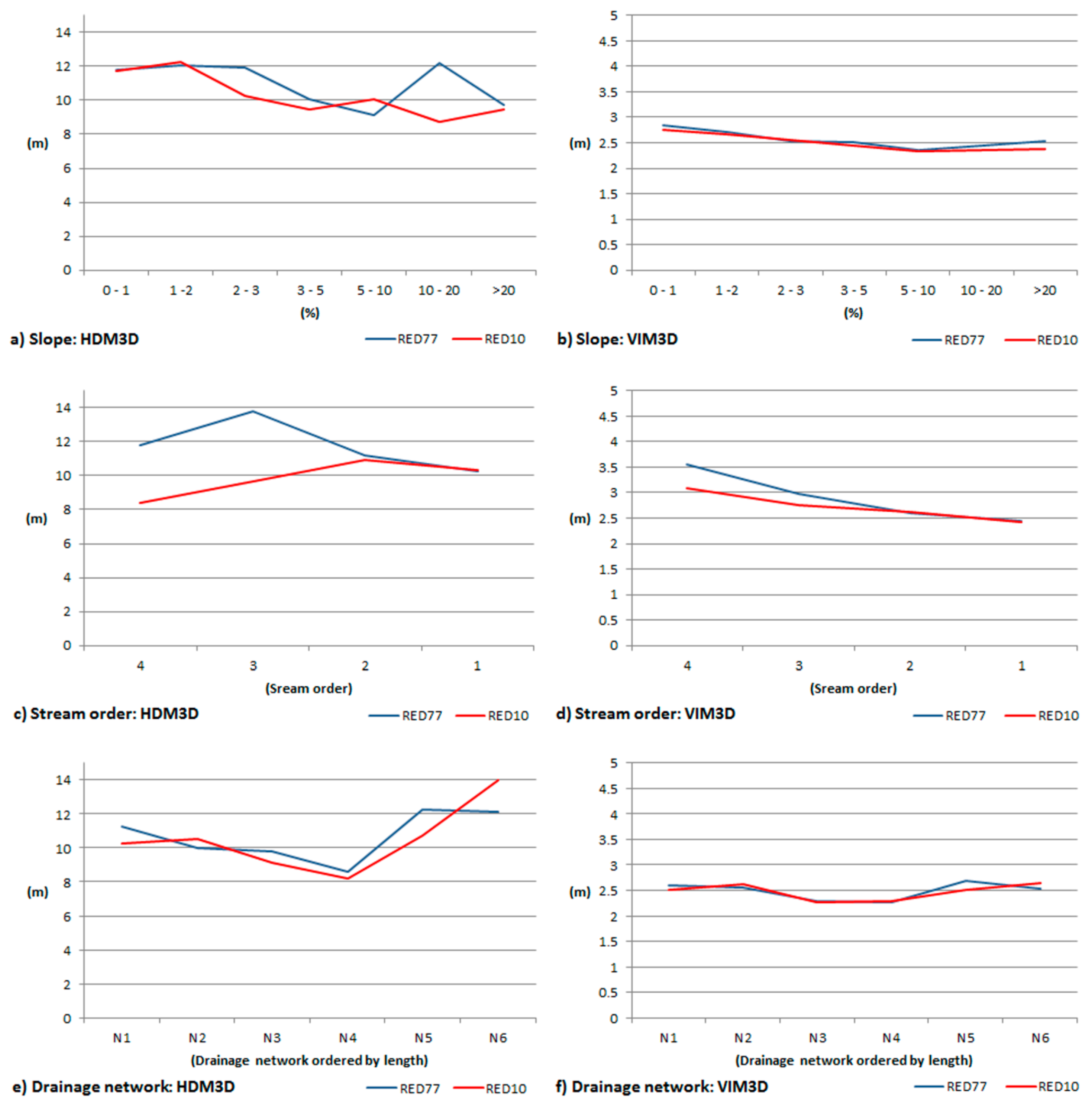
  • Slope (Figure 7a,b): Slope has a great influence on the height error, depending on the planimetric accuracy. In this context, some studies [25,53,54] have analyzed these dependencies between vertical and horizontal errors on contour lines based on the tangent of the slope (by a regression using Koppe’s formula). The values of HDM3D (Figure 7a) show a tendency of reduction of maximum displacements with the slope, although there are some specific cases which show some peaks. We have to note that the results of Hausdorff distance-based methods have a large sensibility to great displacements even though these displacements were restricted to a small section of the linestring. On the other hand, the mean values of displacements analyzed using VIM3D (Figure 7b) show a more uniform behavior with a general reduction of about 20% of displacements with the increase of slopes until the 5–10% case and after that, a stabilization or minor increase of displacements with the slope. This behavior was caused by the planimetric uncertainty of channels in flat zones caused by the algorithm applied in the extraction process.
  • Stream order (Figure 7c,d): In the case of HDM3D, the distribution of the results by stream order shows irregular behavior without clear tendencies. On the other hand, the results of VIM3D show an increase of displacements with the stream order in both datasets, and more specifically of about 40% in the RED77 case and about 25% in the RED10 case. The general trend shown by this method is accorded to the extraction algorithm if we take into account that the axes of channels are supposedly worse-defined with the increase of the stream order because of the geomorphologic conditions of the terrain (flatness).
  • Drainage network (Figure 7e,f): In these cases (HDM3D and VIM3D), there is a similar behavior in both datasets with lower variability of the values obtained. We cannot establish a relationship between the displacement obtained and the distribution of drainage networks applied.
To summarize, analysis by slopes, stream order and drainage network, mainly based on VIM3D values, has allowed the relationship between slope and displacement to be verified. In general, both DEMs have a similar pattern of behavior: the tendency of lines presented in Figure 7. However, RED10 has a clearly better result when analyzed in relation to the stream order (Figure 7a,b). Logically, this is due to the temporal proximity with respect to the reference dataset.
As was described previously, the methodology proposed in this study has allowed us to obtain a general knowledge of the positional behavior of the complete drainage network. However a more detailed analysis is possible when selecting a particular drainage subnetwork or channel. Logically, the results of the displacements obtained must be taken into account as changes in the drainage channel when those values exceed the estimated relative accuracy of the DEMs (shown in Table 1). This value is included in Figure 8 using a buffer of 9.25 m. Otherwise, the lower displacements are not significant. In this study, we have not detected mean displacements of linestrings which achieve this threshold in all cases considered (RED77 and RED10). However, some parts of several linestrings presented greater displacements with respect to the accuracy of the implicated DEMs and can be considered as changes of the drainage channels (caused by evolution in time or by specific errors of the extraction process). The values of the displacements obtained using HDM3D for each linestring can be used to detect these behaviors, because they are related to their maximum displacements. As an example, Figure 8 shows some particular cases of the changes of some channels of case RED77 (RED77 vs. IGN11). The selection of these cases is based on the results obtained from HDM3D (shown in Figure 5). We have to note that, as previously described, the positional assessment was developed from the vertexes of the IGN11 linestrings to the RED77 linestrings. However, in Figure 8, displacement vectors are shown in the inverse direction in order to present the evolution in time. To facilitate the interpretation of the displacements, Figure 8 displays as background two orthoimages obtained from the same source of the DEMs and referred to the same date. More specifically, Figure 8a shows an example of the most common case where the displacements were lower than the relative accuracy between DEMs (RED77 and IGN11) of 9.25 m (a buffer around RED77 channels is displayed in Figure 8 to show the planimetric accuracy). On the other hand, Figure 8b–d show cases where some displacement vectors exceed the relative accuracy between both DEMs, although the mean displacement vector of the line was lower than that value. In these particular cases, the displacements were caused by errors of the DEMRED77 or by problems in the extraction process.
Definitely, the values of displacement obtained using HDM3D and the visual analysis allowed us to detect some particular cases where some sections were not extracted correctly. This could be caused by positional discrepancies of the original DEM or by the extraction process. The particular analysis could also be used to detect significant changes of the channels between several dates (e.g., a multi-temporal analysis). It is interesting to notice that this simple procedure can be used to define two quality indices based on proportions and controlled by a metric tolerance: (1) proportions of incorrectly extracted channels and (2) proportion of channels with considerable change over time.
On the other hand, the general analysis (mainly based on VIM3D) of the drainage channels of RED77 and RED10 showed values of mean displacements lower than the spatial resolution of the original DEMs. In conclusion, we found a good positional behavior of the channels extracted in these examples, considering the presence of some cases where the original DEM or the extraction of channels was not correct.
Previously, when analyzing the distribution functions we described that the 2D and 3D results obtained are similar in both datasets (RED77 and RED10). This aspect confirms that both original DEMs used in this study had a great similarity and accuracy in heights. In this sense, we can conclude that the accuracy of planimetric displacements is limited to the DEMs’ spatial resolution (10 m), and this can be translated into the results of the channel extraction process.

5. Conclusions

This paper describes a new method developed in order to determine the positional displacements of drainage networks extracted from DEMs, and more specifically of drainage channels, by using accuracy assessment methods based on linestrings. The main novelty is the use of these type of elements instead of using points for this purpose. We consider that this aspect is very important because drainage channels are usually represented by linestrings, and logically this assessment is more adequate if carried out using the complete features of the element implicated instead of using solely a sample of discrete positions. In addition to the completeness of this assessment, the use of these elements allows the obtaining of more homogeneous spatial distributions of elements with respect to the samples of points which could be distributed more irregularly.
The method proposed in this study describes several stages for data preparation, including the selection of the drainage channels extracted from DEMs, the obtaining and selection of the linestrings to be used as reference dataset, the editing of the linestrings in order to obtain homologous datasets to be compared and the matching of linestrings between both datasets. Considering the linestring-based assessment methods described until this time in the references, we suggest the use of the HDM3D and the VIM3D in order to determine a maximum and a mean value of displacement, and a mean 3D vector of each channel. Additionally, the 3D vectors which compose the calculation of the VIM3D mean vector could be used for analyzing some sections. The use of 3D methods supposes an important novelty in contrast to those studies of linestrings which are mainly based on 2D analysis. Also, we propose the use of several tools (maps, aggregation of results, new indices, etc.), in order to obtain a wider assessment of positional accuracy, or a time change analysis. To summarize, our approach allows us to determine maximum and mean displacements of drainage channels in 2D, 3D, globally and particularly.
The method has been tested using two datasets of channels extracted from two DEMs. The results have demonstrated the viability of this method in determining the positional behavior of the channels extracted using both local and general values. The analysis was developed at two levels, in general considering the mean value of all channels (the network case) and particularly, considering one selected channel or a section of one channel. In addition, several groups of channels were analyzed taking into account several features such as stream order, drainage network and slope. The results obtained in this study have allowed us to contrast the dependency of the displacements with respect to the stream order and the slope of the terrain. More specifically, the greatest displacements were obtained in the highest stream order values and in the flat zones, which is coherent taking into account the greater uncertainty in the extraction of channels in these zones.
Future research will focus on the reduction of the spatial resolution of DEMs in order to determine temporal changes in the drainage network and the application to zones with different geomorphologies and hydrologic characteristics.

Author Contributions

All authors conceived and designed the study, Antonio T. Mozas-Calvache and Manuel A. Ureña-Cámara performed the experiments. All authors analyzed the results and wrote the paper. All authors read and approved the manuscript.

Conflicts of Interest

The authors declare no conflict of interest.

References

  1. National Aeronautics and Space Administration (NASA). Advanced Spaceborne Thermal Emission and Reflection Radiometer (ASTER) Global Digital Elevation Model Version 2 (GDEM V2). Available online: http://asterweb.jpl.nasa.gov/GDEM.ASP (accessed on 12 June 2017).
  2. Wohl, E. Hydrology: Streams. In River Ecosystem Ecology: A Global Perspective; Likens, G.E., Ed.; Academic Press: San Diego, CA, USA, 2010; pp. 23–31. [Google Scholar]
  3. O’Callaghan, J.F.; Mark, D.M. The extraction of drainage networks from digital elevation data. Comput. Vis. Graph. 1984, 28, 323–344. [Google Scholar] [CrossRef]
  4. Peucker, T.K.; Douglas, D.H. Detection of surface-specific points by local parallel processing of discrete terrain elevation data. Comput. Graph. Image Process. 1975, 4, 375–387. [Google Scholar] [CrossRef]
  5. Jenson, S.K.; Domingue, J.O. Extracting topographic structure from digital elevation data for geographic information system analysis. Photogramm. Eng. Remote Sens. 1988, 54, 1593–1600. [Google Scholar]
  6. Tarboton, D.G.; Bras, R.L.; Rodriguez-Iturbe, I. On the extraction of channel networks from digital elevation data. Hydrol. Process. 1991, 5, 81–100. [Google Scholar] [CrossRef]
  7. Tribe, A. Automated recognition of valley lines and drainage networks from grid digital elevation models: A review and a new method. J. Hydrol. 1992, 139, 263–293. [Google Scholar] [CrossRef]
  8. Soille, P.; Gratin, C. An efficient algorithm for drainage network extraction on DEMs. J. Vis. Commun. Image Represent. 1994, 5, 181–189. [Google Scholar] [CrossRef]
  9. Martz, L.W.; Garbrecht, J. Automated recognition of valley lines and drainage networks from grid digital elevation models: A review and a new method—Comment. J. Hydrol. 1995, 167, 393–396. [Google Scholar] [CrossRef]
  10. Hou, K.; Sun, J.; Yang, W.; Sun, T.; Wang, Y.; Ma, S. Automatic Extraction of Drainage Networks from DEMs Base on Heuristic Search. J. Softw. 2011, 6, 1611–1618. [Google Scholar] [CrossRef]
  11. Federal Geographic Data Committee (FGDC). Geospatial Positioning Accuracy Standards Part 3: National Standard for Spatial Data Accuracy; US Federal Geographic Data Committee: Reston, VA, USA, 1998.
  12. United States Geological Survey (USGS). DEM Standards, 1998. Specifications (Part-2), Standards for Digital Elevation Models, National Mapping Program. Standards; United States Geological Survey: Reston, VA, USA, 1998.
  13. American Society for Photogrammetry and Remote Sensing (ASPRS). ASPRS Positional Accuracy Standards for Digital Geospatial Data. Photogramm. Eng. Remote Sens. 2015, 81, 1–26. [Google Scholar] [CrossRef]
  14. Li, Z. A comparative study of the accuracy of digital terrain models (DTMs) based on various data models. ISPRS J. Photogramm Remote Sens. 1994, 49, 2–11. [Google Scholar] [CrossRef]
  15. Hirano, A.; Welch, R.; Lang, H. Mapping from ASTER stereo image data: DEM validation and accuracy assessment. ISPRS J. Photogramm. Remote Sens. 2003, 57, 356–370. [Google Scholar] [CrossRef]
  16. Miliaresis, G.C.; Paraschou, C.V. Vertical accuracy of the SRTM DTED level 1 of Crete. Int. J. Appl. Earth Obs. 2005, 7, 49–59. [Google Scholar] [CrossRef]
  17. Aguilar, F.J.; Mills, J.P. Accuracy assessment of LiDAR-derived Digital Elevation Models. Photogramm. Rec. 2008, 23, 148–169. [Google Scholar] [CrossRef]
  18. Höhle, J.; Höhle, M. Accuracy assessment of digital elevation models by means of robust statistical methods. ISPRS J. Photogramm. Remote Sens. 2009, 64, 398–406. [Google Scholar] [CrossRef]
  19. Mukherjee, S.; Joshi, P.K.; Mukherjee, S.; Ghosh, A.; Garg, R.D.; Mukhopadhyay, A. Evaluation of vertical accuracy of open source Digital Elevation Model (DEM). Int. J. Appl. Earth Obs. 2013, 21, 205–217. [Google Scholar] [CrossRef]
  20. McMaster, K.J. Effects of digital elevation model resolution on derived stream network positions. Water Resour. Res. 2002, 38, 13–19. [Google Scholar] [CrossRef]
  21. Pirotti, F.; Tarolli, P. Suitability of LiDAR point density and derived landform curvature maps for channel network extraction. Hydrol. Process. 2010, 24, 1187–1197. [Google Scholar] [CrossRef]
  22. Monteiro, E.V.; Carneiro, A.D.F.S.; Fonte, C.C.; de Lima, J.L.; Santos, R.L.R.; Pólo, I.I. Assessing positional accuracy of drainage networks extracted from ASTER, SRTM and OpenStreetMap. In Proceedings of the 18th AGILE International Conference on Geographic Information Science, Lisboa, Portugal, 9–12 June 2015; Bacao, F., Santos, M.Y., Painho, M., Eds.; pp. 1–5. [Google Scholar]
  23. Reinoso, J.F. A priori horizontal displacement (HD) estimation of hydrological features when versioned DEMs are used. J. Hydrol. 2010, 384, 130–141. [Google Scholar] [CrossRef]
  24. Mozas, A.; Ureña, M.A.; Ariza, F.J. Methodology for analyzing multi-temporal planimetric changes of river channels. In Proceedings of the 26th International Cartographic Conference, Dresde, Germany, 25–30 August 2013; Buchroithner, M.F., Ed.; pp. 25–30. [Google Scholar]
  25. Mozas-Calvache, A.; Ureña-Cámara, M.; Pérez-García, J.L. Accuracy of contour lines using 3D bands. Int. J. Geogr. Inf. Sci. 2013, 27, 2362–2374. [Google Scholar] [CrossRef]
  26. Perkal, J. On epsilon length. Bulletin de l’Academie Polonaise des Sciences 1956, 4, 399–403. [Google Scholar]
  27. Chrisman, N.R. A theory of cartographic error and its measurement in digital bases. In Proceedings of the Fifth International Symposium on Computer-Assisted Cartography, Crystal City, Arlington, VA, USA, 22–28 August 1982; Foreman, J., Ed.; pp. 159–168. [Google Scholar]
  28. Blakemore, M. Generalisation and error in spatial data bases. Cartographica 1984, 21, 131–139. [Google Scholar] [CrossRef]
  29. Caspary, W.; Scheuring, R. Positional accuracy in spatial databases. Comput. Environ. Urban. Syst. 1993, 17, 103–110. [Google Scholar] [CrossRef]
  30. Leung, Y.; Yan, J. A locational error model for spatial features. Int. J. Geogr. Inf. Sci. 1998, 12, 607–620. [Google Scholar] [CrossRef]
  31. Shi, W. A generic statistical approach for modelling error of geometric features in GIS. Int. J. Geogr. Inf. Sci. 1998, 12, 131–143. [Google Scholar] [CrossRef]
  32. Shi, W.; Liu, W. A stochastic process-based model for the positional error of line segments in GIS. Int. J. Geogr. Inf. Sci. 2000, 14, 51–66. [Google Scholar] [CrossRef]
  33. Delafontaine, M.; Nolf, G.; Van de Weghe, N.; Antrop, M.; de Maeyer, P. Assessment of sliver polygons in geographical vector data. Int. J. Geogr. Inf. Sci. 2009, 23, 719–735. [Google Scholar] [CrossRef]
  34. McMaster, R.B. A statistical analysis of mathematical measures for linear simplification. Am. Cartogr. 1986, 13, 103–116. [Google Scholar] [CrossRef]
  35. Skidmore, A.K.; Turner, B.J. Map Accuracy Assessment Using Line Intersect Sampling. Photogramm. Eng. Remote Sens. 1992, 58, 1453–1457. [Google Scholar]
  36. Abbas, I.; Grussenmeyer, P.; Hottier, P. Contrôle de la planimétrie d’une base de données vectorielles: Une nouvelle méthode basée sur la distance de Haussdorff: La méthode du contrôle linéaire. Bulletin Societé Française de Photogrammétrie et Télédétection 1995, 137, 6–11. [Google Scholar]
  37. Goodchild, M.F.; Hunter, G.J. A simple positional accuracy measure for linear features. Int. J. Geogr. Inf. Sci. 1997, 11, 299–306. [Google Scholar] [CrossRef]
  38. Tveite, H.; Langaas, S. An accuracy assessment method for geographical line data sets based on buffering. Int. J. Geogr. Inf. Sci. 1999, 13, 27–47. [Google Scholar] [CrossRef]
  39. Mozas-Calvache, A.T.; Ariza-López, F.J. New method for positional quality control in cartography based on lines. A comparative study of methodologies. Int. J. Geogr. Inf. Sci. 2011, 25, 1681–1695. [Google Scholar] [CrossRef]
  40. Mozas-Calvache, A.; Ariza-López, F.J. Adapting 2D positional control methodologies based on linear elements to 3D. Surv. Rev. 2015, 47, 195–201. [Google Scholar] [CrossRef]
  41. Gil de la Vega, P.; Ariza-López, F.J.; Mozas-Calvache, A.T. Models for positional accuracy assessment of linear features: 2D and 3D cases. Surv. Rev. 2016, 48, 347–360. [Google Scholar] [CrossRef]
  42. Mozas, A.T.; Ariza, F.J. Methodology for positional quality control in cartography using linear features. Cartogr. J. 2010, 47, 371–378. [Google Scholar] [CrossRef]
  43. De Jager, A.L.; Vogt, J.V. Development and demonstration of a structured hydrological feature coding system for Europe. Hydrol. Sci. J. 2010, 55, 661–675. [Google Scholar] [CrossRef]
  44. Chen, J.; Lin, G.; Yang, Z.; Chen, H. The relationship between DEM resolution, accumulation area threshold and drainage network indices. In Proceedings of the IEEE 18th International Conference on Geoinformatics, Beijing, China, 18–20 June 2010; Liu, Y., Chen, A., Eds.; pp. 1–5. [Google Scholar]
  45. Strahler, A.N. Hypsometric (area-altitude) analysis of erosional topography. Geol. Soc. Am. Bull. 1952, 63, 1117–1142. [Google Scholar] [CrossRef]
  46. Xavier, E.; Ariza-López, F.J.; Ureña-Cámara, M.A. A survey of measures and methods for matching geospatial vector datasets. ACM Comput. Surv. 2016, 49, 39. [Google Scholar] [CrossRef]
  47. Instituto Geográfico Nacional (IGN). Download Center. Available online: http://centrodedescargas.cnig.es/CentroDescargas/ (accessed on 12 June 2017).
  48. Red de Información Ambiental de Andalucía (REDIAM). Available online: http://www.juntadeandalucia.es/medioambiente/site/rediam (accessed on 12 June 2017).
  49. Instituto de Estadística y Cartografía de Andalucía (IECA). Available online: https://www.juntadeandalucia.es/institutodeestadisticaycartografia (accessed on 12 June 2017).
  50. ESRI. ArcGISTM v10.2 Help Center. Available online: http://resources.arcgis.com/en/help/ (accessed on 12 June 2017).
  51. Mozas-Calvache, A.T.; Ariza-López, F.J. Detection of systematic displacements in spatial databases using linear elements. Cartogr. Geogr. Inf. Sci. 2014, 41, 309–322. [Google Scholar] [CrossRef]
  52. Ariza-López, F.J.; Mozas-Calvache, A.T.; Ureña-Cámara, M.A.; Alba-Fernández, V.; García-Balboa, J.L.; Rodríguez-Avi, J.; Ruiz-Lendínez, J.J. Influence of sample size on line-based positional assessment methods for road data. ISPRS J. Photogramm. Remote Sens. 2011, 66, 708–719. [Google Scholar] [CrossRef]
  53. Gustafson, G.C.; Loon, J.C. Contour accuracy and the National Map Accuracy Standards. Surv. Mapp. 1982, 42, 385–402. [Google Scholar]
  54. Imhof, E. Cartographic Relief Presentation; ESRI Press: Redlands, CA, USA, 2007. [Google Scholar]
Figure 1. Proposed methodology.
Ijgi 06 00234 g001
Figure 2. Characteristics of the zone of study (National Topographic Map of Spain (MTN): sheet 946) based on DEMIGN11 and vector source (VCT).
Ijgi 06 00234 g002
Figure 3. Obtaining of IGN112A dataset: (a) General view of IGN111 and VCT datasets; (b) General view of IGN111 and IGN112A dataset; (c) Detailed view of IGN111 and VCT datasets; (d) Detailed view of IGN111 and buffer of VCT dataset; (e) Detailed view of IGN111 and IGN112A datasets.
Ijgi 06 00234 g003
Figure 4. Distribution functions of Hausdorff distance method (HDM) and Vertex Influence Method (VIM) general results: (a) HDM2D; (b) HDM3D; (c) VIM2D and (d) VIM3D.
Ijgi 06 00234 g004
Figure 5. Results of Hausdorff Distance (HDM3D).
Ijgi 06 00234 g005
Figure 6. VIM3D Displacement vectors (modules are multiplied by 200).
Ijgi 06 00234 g006
Figure 7. Results of HDM3D and VIM3D segmented by: (a,b) slopes; (c,d) stream order; (e,f) drainage network.
Ijgi 06 00234 g007
Figure 8. Examples of mean displacement vectors obtained in case RED77 vs. IGN11 (labels: Z increment).
Ijgi 06 00234 g008
Table 1. Datasets used in this study.
TypeNameSourceFeaturesUse
DEMDEMRED77B&W Flight S18k, year 197710 × 10 mSource for RED77
P-RPA95% 1 = 9.253 m
Z-RPA95% 2 = 0.406 m
DEMDEMRED10Digital Flight, year 201010 × 10 mSource for RED10
P-RPA95% 1 = 9.178 m
Z-RPA95% 2 = 0.201 m
DEMDEMIGN11Digital Flight, year 20115 × 5 mSource for IGN11
LinestringsRED77DEMRED77 To be assessed
LinestringsRED10DEMRED10 To be assessed
LinestringsIGN11DEMIGN11 Reference
LinestringsVCTVector source at scale 10,000 Selection mask
1 P-RPA95%: Planimetric relative positional accuracy in relation to DEMIGN11 at 95% of confidence; 2 Z-RPA95%: Height relative positional accuracy in relation to DEMIGN11 at 95% of confidence. Note: Relative positional accuracies calculated following the FGDC [11] standard using a sample of 50 points.
Table 2. General results obtained in this study.
DatasetHDM2D (m)HDM3D (m)VIM2D Displ. (m)VIM3D Displ. (m)VIM3D dX (m)VIM3D dY (m)VIM3D dZ (m)
RED77 (mean)10.82510.8542.5052.549−0.038−0.1490.053
RED10 (mean)10.30510.3422.4522.4950.044−0.1960.128
RED77 (s)7.2357.2450.9360.9530.7690.7360.234
RED10 (s)5.3205.3110.8020.8160.6990.7080.242
p-value0.2820.2890.4240.4460.1420.3923.88×10−5

