A Hierarchical Approach for Measuring the Consistency of Water Areas between Multiple Representations of Tile Maps with Different Scales

Abstract

In geographic information systems, the reliability of querying, analysing, or reasoning results depends on the data quality. One central criterion of data quality is consistency, and identifying inconsistencies is crucial for maintaining the integrity of spatial data from multiple sources or at multiple resolutions. In traditional methods of consistency assessment, vector data are used as the primary experimental data. In this manuscript, we describe the use of a new type of raster data, tile maps, to access the consistency of information from multiscale representations of the water bodies that make up drainage systems. We describe a hierarchical methodology to determine the spatial consistency of tile-map datasets that display water areas in a raster format. Three characteristic indices, the degree of global feature consistency, the degree of local feature consistency, and the degree of overlap, are proposed to measure the consistency of multiscale representations of water areas. The perceptual hash algorithm and the scale-invariant feature transform (SIFT) descriptor are applied to extract and measure the global and local features of water areas. By performing combined calculations using these three characteristic indices, the degrees of consistency of multiscale representations of water areas can be divided into five grades: exactly consistent, highly consistent, moderately consistent, less consistent, and inconsistent. For evaluation purposes, the proposed method is applied to several test areas from the Tiandi map of China. In addition, we identify key technologies that are related to the process of extracting water areas from a tile map. The accuracy of the consistency assessment method is evaluated, and our experimental results confirm that the proposed methodology is efficient and accurate.

1. Introduction

Five essential dimensions regarding a possible geospatial data standard, including the positional accuracy, attribute accuracy, logical consistency, completeness, and lineage, were proposed in the 1980s [1]. These five dimensions eventually formed the basis for defining data-quality elements. Logical consistency is a crucial element of spatial data quality [2]; thus, maintaining the consistency of spatial data is very important for aspects, including the high-speed transmission of spatial data on the Internet [3], querying spatial data at multiple resolutions [4], and extracting and integrating information from spatial data with varying levels of detail [5]. In particular, interest in volunteered geographic information (VGI) has rapidly increased in recent years [6]. An official spatial dataset can be considerably different from a VGI dataset. The integration of VGI data (e.g., OpenStreetMap) and official data is an important issue for many applications such as data-description enrichment [7,8], data-quality enhancement [9], and data-change detections. However, the consistency of geographical objects at different scales must be assessed and maintained when integrating spatial data. Therefore, additional attention should be paid to the consistency of spatial data with the rapid development of computational power and the Internet.

Previous methods of consistency assessment can be classified into two categories [10], specifically object-based consistency [11,12,13,14] and relation-based consistency [15,16,17,18,19,20,21]. Object-based consistency mainly involves the similarity of shapes, structures, and dimensions of geographical objects at different levels of detail. Dettoriet et al. [11] assessed the geometrical consistency of spatial objects under the influence of a simplification operator. Delis et al. [12] proposed a framework to evaluate the geometrical consistency of line elements between two map layers. Du et al. [13] proposed a model to assess the structural consistency of complex regions. In this approach, the closest structure-level graph is used to form multiple potential representations of complex regions. Generalization operators are then used to automatically generate correspondences at different scales. Finally, the correspondences are used to assess the structural consistency of spatial objects at different levels of detail. Relation-based consistency mainly considers the similarity of relative sizes, directional relationships, and topological relationships among geographical objects at different scales and resolutions. Egenhoferet et al. [15] developed a framework to assess the topological consistency at different levels of detail based on topological homeomorphism. Tryfona and Egenhofer [16] evaluated the topological consistency of spatial objects at different scales by considering homogeneous and heterogeneous networks and proposed a framework to drive topological relationships among aggregates from the relationships among the components. Du et al. [19] proposed computational measures to derive the directional relationships between spatial objects on a coarse level using the relationships among spatial objects at a detailed level. The consistency of the directional relationships among these multiple representations can then be assessed by determining whether the derived relationships match those established from the multi-resolution spatial objects at a coarse level. Andrea et al. [20] developed methods to assess the degree of violation of a topological dependency constraint using geometries stored in a spatial-database instance. Brisaboa et al. [21] developed a method to measure the inconsistency of spatial datasets with respect to a set of topological constraints that should be maintained between the spatial objects in the dataset.

Studies of similarity calculations for area elements have mainly considered the shape similarity factor. Global indicators for shape measurement such as the perimeter, size, convex perimeter, compactness, roughness, and elongation can be used to measure degrees of similarity between objects [22]. Fourier descriptors are also widely used to calculate the shape similarity [23] because these factors are invariant to starting point shifts in the polygon curve. In addition, similarities have been measured by using complex methods (e.g., computational geometry [24], polygon curve representations [25], the morphological characterization method [26], and the correspondence of visual parts [27]).

The above information indicates that most studies have used vector data to access the consistency of spatial data, whereas few studies have used raster data. However, data sources and GIS types can vary in the context of big data. Extracting meaningful information from a growing collection of unstructured data (e.g., pictures, street views, 3D models, and videos) is necessary but challenging. Therefore, we must use a new form of raster data, namely tile maps, to measure the consistency of representations of water features.

In contrast, the scale of spatial data tends to be the same or at an adjacent scale, and multiscale spatial data are relatively rarely addressed in the studies discussed above. However, spatial data can be generated at a lower resolution using different generalization operators such as simplification, smoothing, aggregation, omission, and displacement [28]. Therefore, multi-resolution spatial data always contain inconsistencies in their topological, directional, and metric relationships because of differences in the measurement methods, data acquisition approaches, and map-generalization algorithms. Consistency assessment methods used at individual scales are not appropriate for multiscale cases. Thus, a new method is required to verify such inconsistencies.

Inconsistencies must be identified before they can be corrected, and such inconsistencies can help identify potentially problematic areas that require the collection of additional data or characterize the degree of certainty associated with information [29]. However, whether such differences occur normally due to the generalization algorithms or because of the presence of erroneous or outdated data in a given database must be determined to make the best use of these inconsistencies [30,31,32,33]. Therefore, prior to the inconsistent processing of spatial data, we must determine the degree of inconsistency present in the data and determine whether the inconsistencies are reasonable or problematic in order to better address inconsistent data in future work. For example, Figure 1 shows two lakes that are inconsistently represented among the multiple scales. Lake A appears at levels 10 and 12, but it disappears at level 11. This inconsistent representation of lake A is unreasonable because its expression is discontinuous. Lake B displays an abrupt change from level 9 to level 10. As the changes between adjacent scales should be progressive, this kind of inconsistency has a negative effect on the acceptance of geographic information by users and their reasoning about that information. We must therefore identify types of inconsistencies that are reasonable or unreasonable to avoid placing unnecessary cognitive burdens on the user and to provide better geographic information services for public use.

Therefore, this paper uses new unstructured tile data to detect inconsistencies in multiscale representations of water areas. We also grade the degrees of inconsistency in a hierarchical manner. Following this introduction, Section 2 describes the hierarchical framework of the inconsistency assessment method for multiscale representations of water areas based on tile data. In Section 3, we describe the methods used to perform feature description, feature extraction, and comparisons at each level. Section 4 presents the results of the experiments, illustrates the proposed approaches, and provides a discussion and analysis of these approaches. Section 5 presents the conclusions.

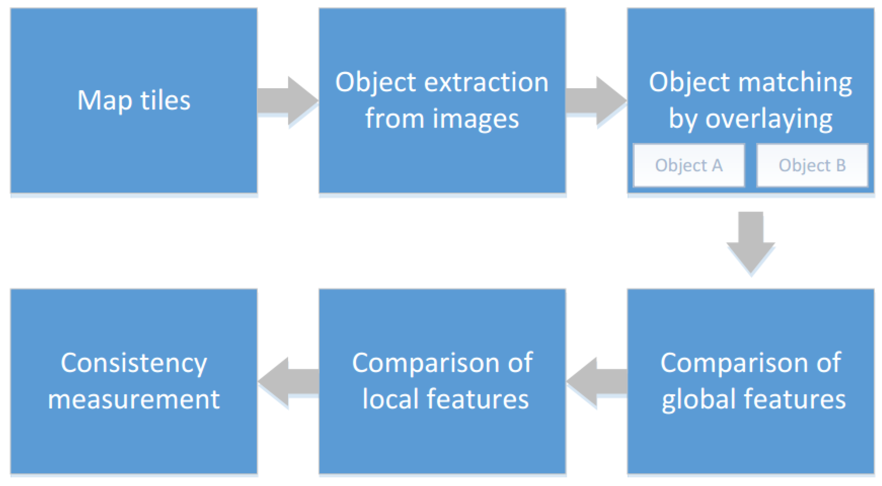
2. Framework of Hierarchical Consistency Assessment for Water Areas

To address the problems outlined above, we must consider the inconsistencies that occur among multiple scales rather than two uniform or adjacent scales. Methods of distinguishing and grading inconsistency information from multiscale spatial data must be determined. In this manuscript, we hierarchically use both global and local features of images to analyze and study this problem.

Fundamentally, the features that are extracted from the images can be divided into two types: global features and local features. The features within images can also be referred to as descriptors. Global descriptors can be used for object detection, object classification, or image retrieval, whereas local descriptors are widely used for object identification or recognition. Global features describe the image as a whole and can generalize the entire object using a single vector, whereas local features describe image patches of an object and are usually expressed in the form of key points. Global and local features provide different types of information about images because of the differences in the computing methods of the two representations. Global features typically include shape descriptors, texture features, and contour representations, whereas local features represent textures in an image patch.

Water areas are expressed in the form of map tiles in this study; thus, we combined local and global features to measure the similarity of match objects. During comparisons, the general features are extracted and compared, and the detailed features are then considered. This approach or method for resolving a problem from the general to the specific or from the whole to the part is referred to as a hierarchical method. A combination of global and local features improves the accuracy of similarity calculations and provides an effective method to grade the degree of consistency.

The basic principle of feature comparison is shown in Figure 2. Let us assume that we have an object S and must select the most similar object to S from objects a, b, and c. When our brain begins to screen, objects that are not similar in appearance, such as object c in this case, are preferentially ignored. This process can be regarded as the analysis and comparison of general features on a global level. After performing a preliminary selection of objects a and b, we must further identify the most similar object from objects a and b. Naturally, we focus on the detailed features of objects a and b. This process can be regarded as an analysis and comparison of detailed features at a local level. Finally, we select object a as the best choice.

In this study, when comparing two matching targets and measuring their consistency, we analyze the global features first, followed by the local features. The degree of consistency is measured and graded according to the feature similarities of the two levels.

Framework for Measuring Consistency

In 2005, Google Maps began to provide global electronic map services, and an increasing number of map services began to adopt tile technologies, including Google Maps, OpenStreetMap, and Bing Maps. These mature commercial tiled map services have common characteristics, including the coordinate system (WGS84), projection (Mercator), image size (256 × 256), image formats (.png and .jpg), and organization rules (pyramid) that they use. Therefore, we divide the proposed method into five components (object extraction, object matching, feature comparison and analysis, and consistency measurement), which are shown in Figure 3, to treat tile data as a potential object of consistency assessment.

(1) Object Extraction

Water extraction involves the separation of water elements from a tile map. As tile technologies have become increasingly advanced, many map suppliers have begun to treat drainage systems as independent elements, and water areas can be directly extracted from map services (e.g., the Tiandi map for China). However, considering the problems of technological universality, the extraction of water from tile elements remains a problem that cannot be ignored. Water is a key component of tile maps and typically has a uniform blue colour within the same map. Thus, image threshold segmentation methods represent the simplest and most effective means of extracting water areas. To obtain more satisfactory extraction results, certain mature tools such as noise removal algorithms and fracture repair algorithms are also applied to extract water areas from map tiles in this study. We do not focus heavily on these tools in this paper.

(2) Object Matching

We match the drainage system by overlaying tile data of different levels. The tile data are organized in a pyramid shape. At the smallest scale, the Earth is shown as one image at 256 pixels by 256 pixels. When the zoom level is increased, the quantity of images increases four-fold, following a given pattern, as shown in Figure 4. Therefore, magnification at a high level must only be performed four times to match the water area and overlay it with low-level tiles from the same coordinate system. Overlapping water elements can be treated as targets with the same name.

(3) Object Feature Comparison

Studies that have evaluated object-based consistency have mainly considered two factors: the shapes and structures of spatial objects. Scholars have always considered shapes, sizes, perimeters, convex perimeters, and other indicators when using traditional methods of feature comparisons that are based on vector data. However, coordinate data rather than image data have been used when measuring these indicators. Therefore, we compare the features of water areas via image processing. If the level of detail exceeds a certain threshold, a greater number of viewable objects corresponds to fewer objects that can be expressed [34]. Features are compared based on the global structures of shapes, and local similarity criteria are used to further refine the comparisons. Multi-level features of area objects, which include global features and local features, are extracted, and improved algorithms are applied. Differences can be easily identified and evaluated when comparing the features of area objects.

(4) Consistency Measurement

From an engineering perspective, the concept of multiple representations is redundant. Thus, a method that can assess and measure the consistency of a database in order to better distinguish between reasonable and unreasonable inconsistencies is needed. Studies that compare maps or databases must explicitly manage fuzziness or uncertainty, partly because of the presence of inconsistencies within the data [35]. Therefore, we grade the fuzziness or uncertainty of inconsistencies that are identified by comparing features in this section. The inconsistencies in multiscale representations of water areas are divided into five grades: exactly consistent, highly consistent, moderately consistent, less consistent, and inconsistent.

3. Measuring the Consistency of Water Areas

3.1. Feature Classification and the Degree of Consistency

A picture is a two-dimensional signal that includes different frequency components. Typically, a region that shows minor changes in brightness includes low-frequency components, which describe a broad range of information. A region that presents drastic changes in brightness such as the edge of an object includes high-frequency components, which describe detailed features. Accordingly, high frequencies provide detailed information about a picture, whereas low frequencies provide the framework of a picture. Thus, we use both general and detailed information to measure the consistency of water areas in this paper.

3.1.1. Degree of Global Feature Consistency

At the International Conference on Image Processing in 1996, Schneider and Chang [36] advanced the concept of image hashes. Subsequently, research on the theory and application of image hashes quickly raised concerns. Many algorithms for generating image hashes have also been proposed [37,38,39]. In pictures, high frequencies provide detailed information, whereas low frequencies reveal structures. The average hash algorithm mainly takes advantage of the low-frequency information in pictures; therefore, we use the improved average hash algorithm to extract features of water areas using the following steps.

(1)

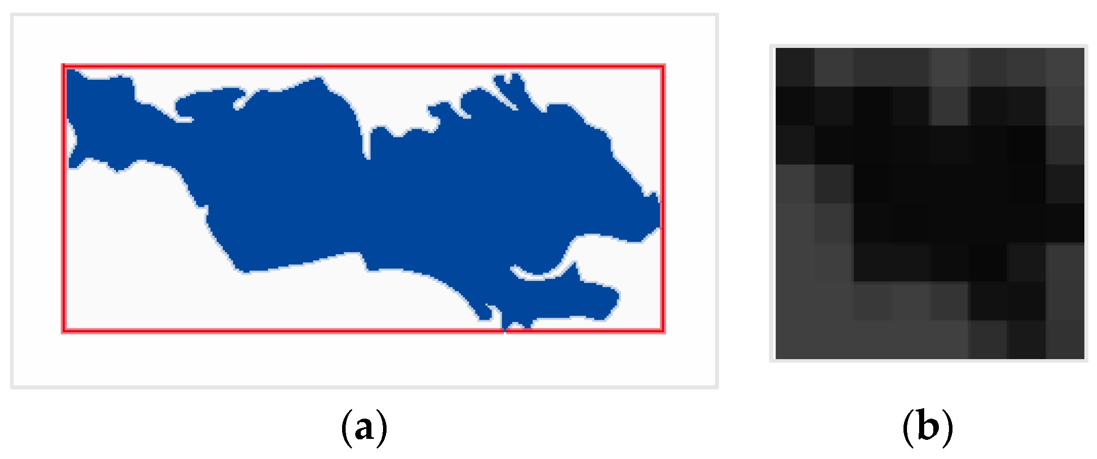
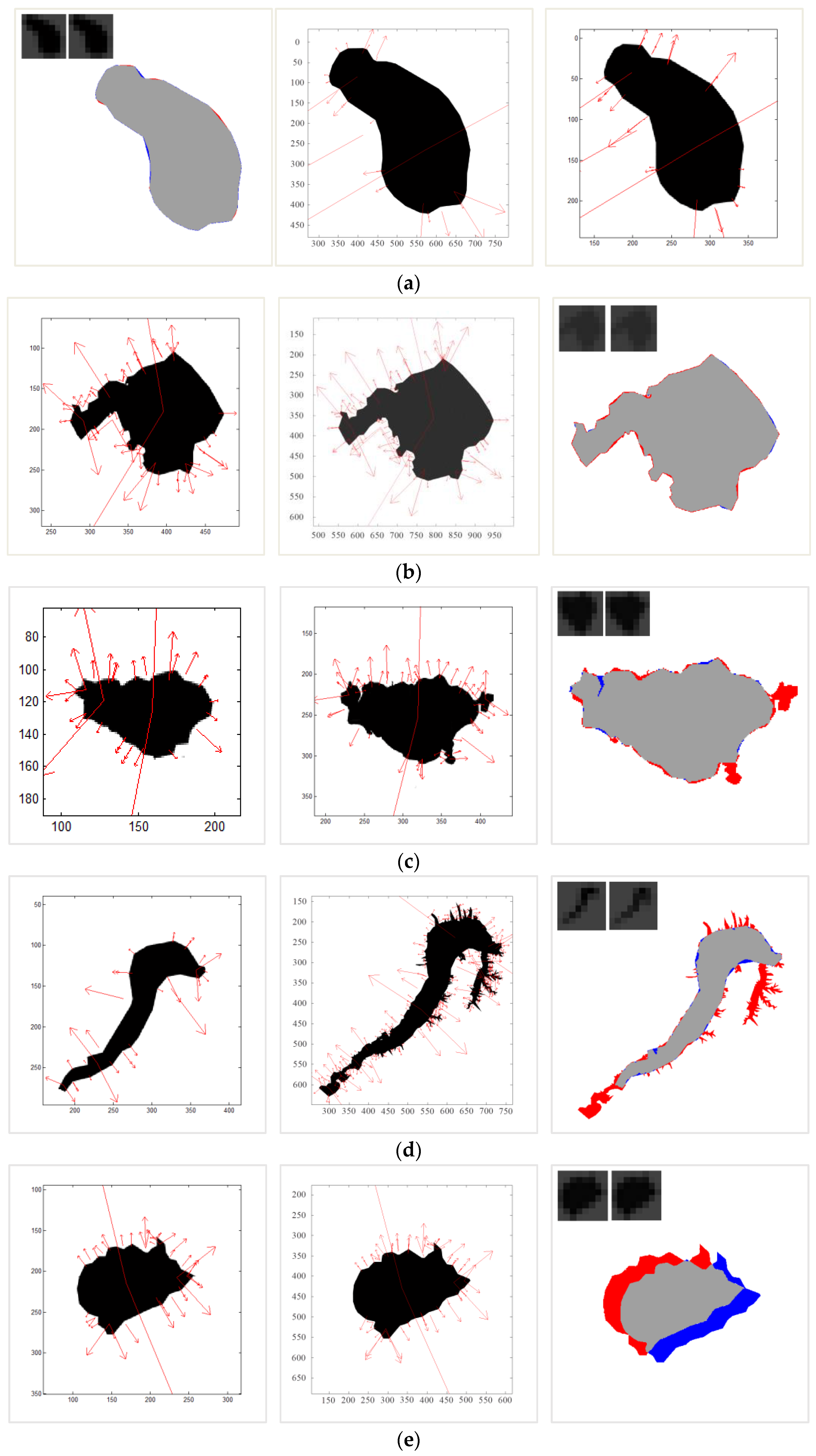
Determine the calculation region. A reasonable calculation region should be identified before feature extraction. In this paper, we consider the minimum bounding rectangle of the object to be the effective calculation region, as shown in Figure 5a.

(2)

Reduce the size. Shrinking is performed to retain sketchy information and remove the high frequencies in an image. In this circumstance, we shrink the image to 8 × 8, yielding a total of 64 pixels. The aspect ratio does not need to be maintained, and features can be condensed to fit into an 8 × 8 square. Thus, the hash algorithm can be applied to assess any changes in the image without considering the scale or aspect ratio.

(3)

Reduce and average the colours. A small 8 × 8 picture is transformed to a grayscale image, as shown in Figure 5b, and the average gray value of the 64 pixels is calculated.

(4)

Calculate the bits. Each bit is characterized depending on whether its colour value is above or below the mean.

(5)

Construct the hash. The 64 bits are set to a 64-bit integer. The order does not matter, as long as consistency is maintained. For example, bits can be set from left to right or from top to bottom using the big-endian approach.

The results of the average hash algorithm remain the same when the aspect ratio of the image changes or the image is scaled. In addition, altering the colours, the brightness, or even the contrast of the image does not remarkably influence the hash value. Thus, this method is efficient.

Let us assume that $h_1$ and $h_2$ are the hash sequences of two images and $n$ is the length of this sequence. Let $h_1\left(i\right)$ and $h_2\left(i\right)$ represent the ith element ($1\le i\le n$) of sequences $h_1$ and $h_2$, respectively. $D\left(h_1,h_2\right)$ represents the similarity between $h_1$ and $h_2$. In this paper, we use the Hamming distance to calculate the degree of similarity. The formula for the similarity is as follows:

$$D\left(h_1,h_2\right)={\displaystyle \sum }_{i=1}^n|h_1\left(i\right)-h_2\left(i\right)|$$

Images with shorter Hamming distances show fewer differences. Conversely, images with greater Hamming distances show more differences. To identify the differences between two images, the hash from each image should be constructed, and the number of bit positions that are different should be counted; this number equals the Hamming distance. A distance of zero indicates that the pictures are completely similar or the same. A distance of 5 indicates that the pictures are likely similar, although a few features may be different from each other. A distance of 10 or more indicates that the pictures are probably different.

We define the degree of global consistency (GC) through our comparison of global features, as follows:

$$GC=\{\begin{array}{c}\frac{10-D\left(h_1,h_2\right)}{10}, D\left(h_1,h_2\right)\le 10\\ 0, D\left(h_1,h_2\right)>10\end{array}$$

when $GC=1$, the two objects are completely consistent in terms of their global features. As GC decreases, the two objects become progressively less consistent. When $GC=0$, the two objects are inconsistent in terms of their global features.

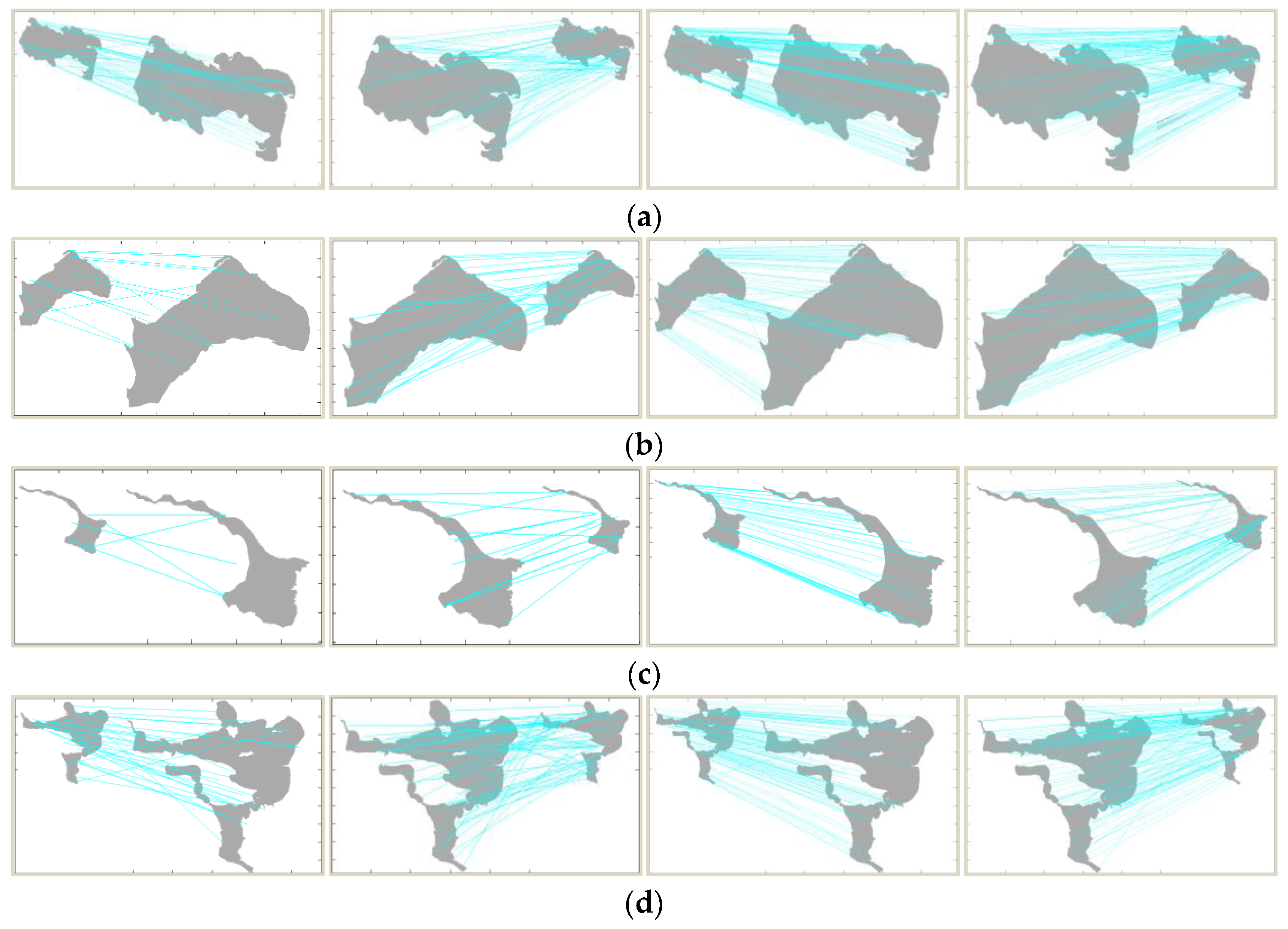
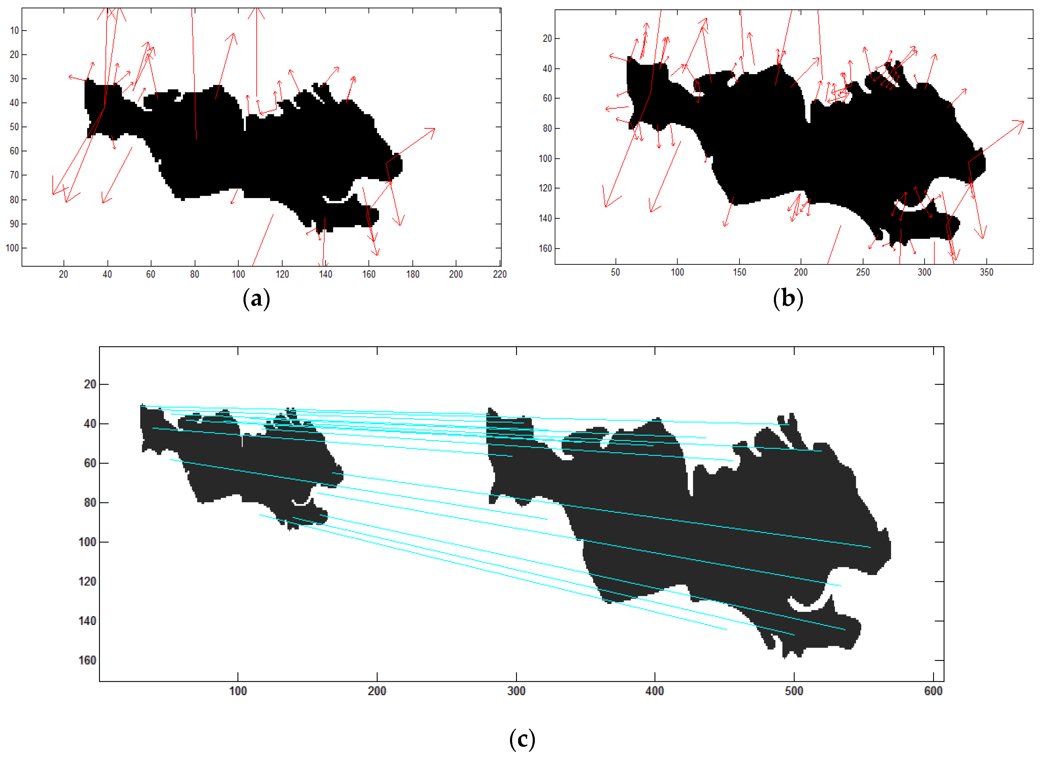
3.1.2. Degree of Local Feature Consistency

The points of interest associated with any object in an image can be extracted to generate a ‘feature description’ of that object. This description, which is extracted from a training image, can then be used to recognize the object when attempting to locate it in a test image that contains many other objects. Even if the scale, noise, and illumination of the image change, the features that are extracted from the training image must be detectable to perform reliable identification. Such points are typically located in high-contrast regions in images (e.g., along the edges of object).

The scale-invariant feature transform (SIFT) is an effective feature descriptor to extract and describe local features in images. The SIFT algorithm was patented in the US by the University of British Columbia and was first published by David Lowe in 1999 [40]. David Lowe perfected SIFT in 2004 [41]. SIFT is the most robust local feature descriptor that can be used for object matching and recognition, and it works by extracting distinctive invariant features. The features are invariant to the image scale and rotation and facilitate robust matching across a substantial range of affine distortion levels, changes in 3D viewpoints, additions of noise, and changes in illumination.

Thus, we attempt to use the SIFT algorithm to measure local features in this study. A typical example is illustrated in Figure 6. A lake from a low level in the Tiandi map is shown in Figure 6a, and the red section is a local SIFT feature. Figure 6b shows the same lake from a high level in the Tiandi map, and the red section is also a local SIFT feature. As shown in these images, 37 keypoints are located in the lake shown in Figure 6a, whereas 93 keypoints are located in the lake shown in Figure 6b. More details of the image are shown when a larger scale is used. Figure 6c shows the matching results; the 22 matching keypoints are connected with green lines. We believe that the presence of a greater number of keypoints that are matched with objects indicates a greater degree of consistency among the matching objects.

When the keypoints of two images are matched, the Euclidean distance of the feature vector of keypoints is used to measure the similarities between the keypoints. The best candidate match for each keypoint is found by identifying its nearest neighbor in the database of keypoints from the training images. However, many feature points in the image might be assigned an incorrect match in the training database because of background noise or similar features. Therefore, a more effective measure is obtained by comparing the distance of the closest neighbor to that of the second-closest neighbor. Lowe rejects all matches for which the distance ratio is greater than 0.8 [41]. In Figure 6c, the ratio is 0.5, and this process performs well because false matches are not observed. Incorrect matches may occur when the ratio is greater than 0.5. More errors occur with larger ratios.

Let $\alpha$ represent the percentage of matches and total keypoints in one image, and let $\beta$ represent the percentage of matches and total keypoints in another image. We define the degree of local consistency (LC) through the comparison of local features as follows:

$$LC=\left(\mathsf{\alpha }+\beta \right)/2$$

If $LC=1$, then the two objects are completely consistent in terms of their local features. As LC decreases, the consistency between two objects becomes progressively weaker. When $LC=0$, the two objects are inconsistent in terms of their local features.

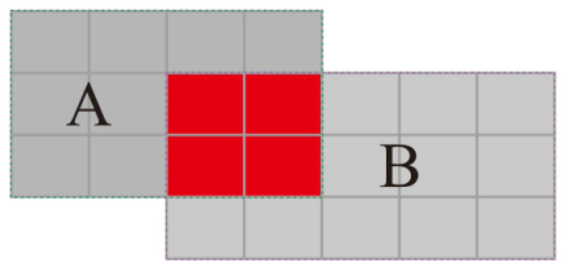
3.1.3. Degree of Overlap

The average hash and SIFT algorithms can be used to measure global and local similarity. However, these methods cannot be used to assess the differences in the positioning of an image. Therefore, we use a third feature index, namely the degree of overlap, to measure this aspect of the differences between images. To a certain degree, the degree of overlap between two images reflects the degree of similarity between the images, although this degree of similarity is not properly conveyed when only the degree of overlap is used. However, we can use the degree of overlap to identify differences in location when the global and local features are similar.

For each group of matching objects in water areas, the degree of overlap OD is the ratio between the overlapping pixel number $Nu{m}_{lap}$ and the total pixel number $Nu{m}_{all}$ after overlaying; specifically, $OD=Nu{m}_{lap}/Nu{m}_{all}$. As shown in Figure 7, area A is composed of 12 pixels, and area B is composed of 15 pixels. The overlapping portions of areas A and B are shown in red. Therefore, the OD of A is $O{D}_A=Nu{m}_{lap}/Nu{m}_{all}=4⁄12=33.3\%$ and the OD of B is $O{D}_B=Nu{m}_{lap}/Nu{m}_{all}=4/15=22.7\%$.

Let $\mathsf{\alpha }$ represent the OD of one image, and let $\mathsf{\beta }$ represent the OD of the other matching image. We define the OD of the two matching objects as follows:

$$OD=\left(\mathsf{\alpha }+\beta \right)/2$$

when $OD=1$, the two objects overlap completely. As OD decreases, the consistency of the two objects becomes increasingly weaker. The OD can be considered to be a strengthening index with the exception of the degree of global feature consistency and the degree of local feature consistency, when the degree of similarity between two objects is finally confirmed.

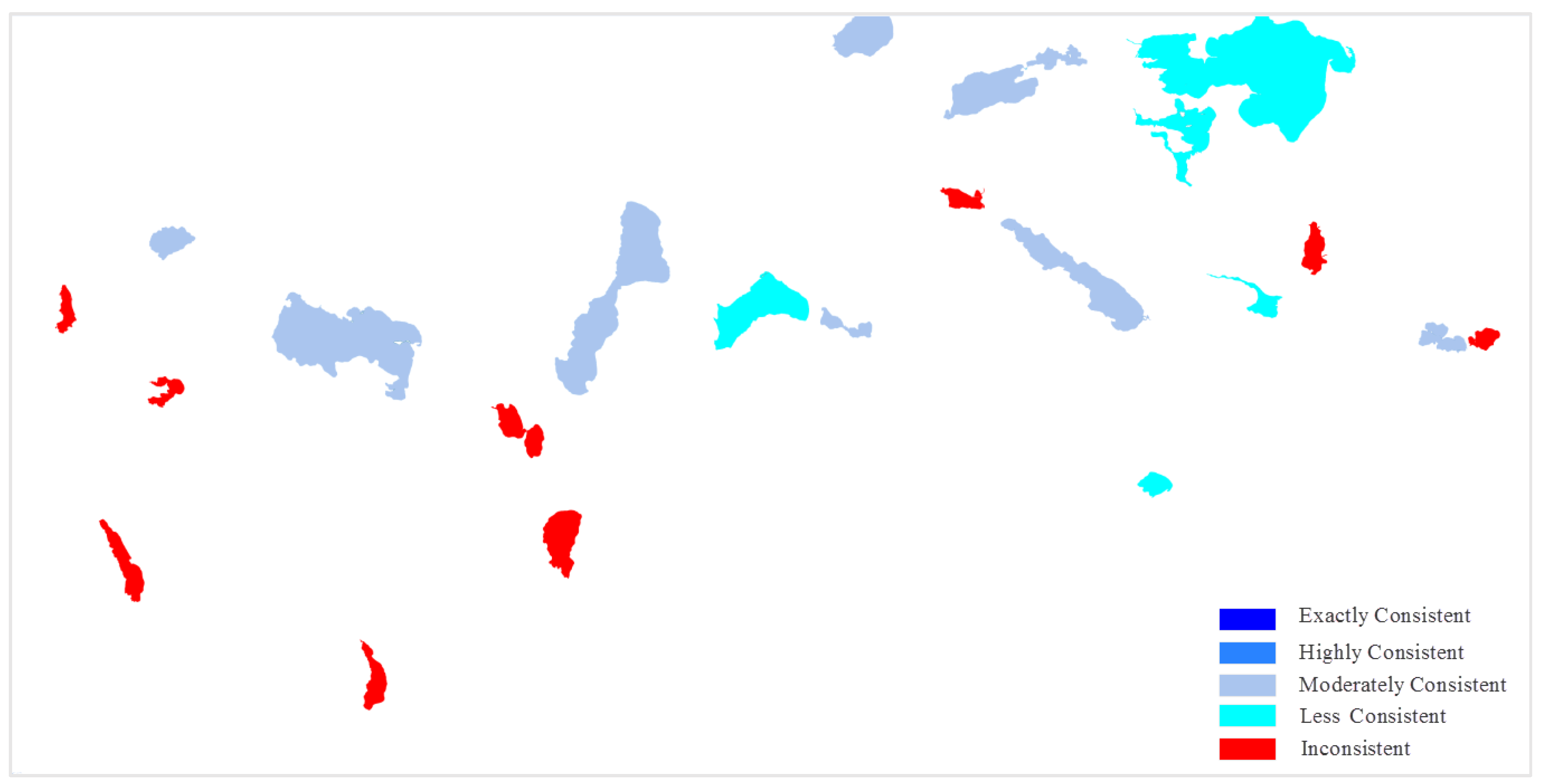
3.2. Definition of Degrees of Consistency

The degree of consistency of two objects can be divided into five grades (exactly consistent, highly consistent, moderately consistent, less consistent, and inconsistent) through the analysis of global and local features, as shown in the following table (

Table 1. Definition of degrees of consistency.

	$0.9\le \mathit{G}\mathit{C}\le 1$	$0.8\le \mathit{G}\mathit{C}<0.9$	$0.7\le \mathit{G}\mathit{C}<0.8$	$0.5<\mathit{G}\mathit{C}<0.7$	$0\le \mathit{G}\mathit{C}\le 0.5$
$0.7\le \mathit{L}\mathit{C}\le 1$	Exactly consistent	Highly consistent	Moderately consistent	Less consistent	Inconsistent
$0.5\le \mathit{L}\mathit{C}<0.7$	Highly consistent	Moderately consistent	Less consistent	Inconsistent	Inconsistent
$0.4\le \mathit{L}\mathit{C}<0.5$	Moderately consistent	Less consistent	Inconsistent	Inconsistent	Inconsistent
$0.2<\mathit{L}\mathit{C}<0.4$	Less consistent	Inconsistent	Inconsistent	Inconsistent	Inconsistent
$0\le \mathit{L}\mathit{C}\le 0.2$	Inconsistent	Inconsistent	Inconsistent	Inconsistent	Inconsistent

).

After calculating the three characteristic indices (the degree of global consistency, the degree of local consistency, and the degree of overlap), we define the consistency between two matching objects via a weighted summation method. This equation can be written as follows:

$$C=\alpha ·GC+\beta ·LC+\gamma ·OD$$

In this equation, $GC$ denotes the global degree of consistency, $LC$ denotes the local degree of consistency, $OD$ denotes the degree of overlap, and $\alpha$, $\beta$, and $\gamma$ are the weighted coefficients. Global features typically have a stronger effect than local features; thus, $\alpha >\beta >\gamma$ and $\alpha +\beta +\gamma =1$. When the precision is 0.1, there are only four possible combinations of the values of $\alpha$, $\beta$, and $\gamma$. To reasonably distinguish the differences between the global and local features and to avoid permitting the strengthening index to have excessive influence, we set $\alpha =0.6$, $\beta =0.3$, and $\gamma =0.1$.

The following figures show typical examples.

As shown in Figure 8, the three indices (the degree of global consistency, the degree of local consistency, and the degree of overlap) of the lakes in a and b are higher; thus, their degree of consistency is identified as highly consistent. The grade of the lake shown in c shows a higher degree of global consistency and a lower degree of local consistency and is identified as less consistent. The lake in d shows a lower degree of both global consistency and local consistency, and is identified as inconsistent. Different changes can lead to different degrees of consistency. When the difference in the global degree of consistency is small, a higher local degree of consistency corresponds to higher overall consistency. When the difference in the local degree of consistency is small, a higher global degree of consistency corresponds to higher overall consistency. We conducted an experiment based on the characteristics of the SIFT algorithm and concluded that the local similarities of two objects are more prominent when the local degree of consistency is greater than 0.5 (Figure 8a). Objects with smoother boundaries correspond to fewer SIFT feature points. Boundaries that are more strongly curved correspond to a higher number of SIFT feature points (Figure 8d). When the global and local degrees of consistency of two objects are roughly the same (e.g., because they are displaced relative to one another), we can further identify the consistency degree using the degree of overlap (Figure 8e). Overall, the degree of consistency of two objects is determined from three indices: the degree of global consistency, the degree of local consistency, and the degree of overlap.

The consistency over multiple scales can be obtained via the accumulation of degrees of consistency for two adjacent scales, which can be represented as follows:

$$C_{multiple}={\displaystyle \sum }_{i=0}^n{C}_i$$

where $C_i$ denotes the degree of consistency between two adjacent scales.

4. Experiments and Analysis

4.1. Methods

The difficulties that are associated with extracting water from tile elements cannot be ignored. Therefore, we focus on methods of extracting independent water areas from a tile map prior to change detection. In contrast to the other elements on a map, water areas are typically expressed as a uniform blue. Therefore, water areas can be separated from other geographical elements shown on a single map using a given colour threshold. However, the extracted water areas display obvious fractures or ‘holes’ due to the overlays from other elements on the map such as roads and annotations. Based on these two factors, this paper proposes the following steps to extract water areas from a tile map.

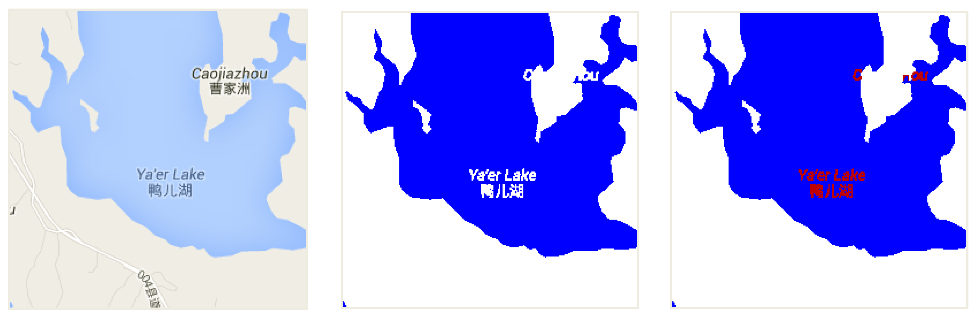
4.1.1. Extract Water Areas via Colour Segmentation

Although the water areas across different tile maps vary in colour, the colour of water on a given map is uniform. Therefore, water elements can be separated from other geographical elements on the same map by using a specific colour threshold. In Figure 9, a tile from the Tiandi map is shown on the left, and the result after extraction with the colour threshold is shown on the right. The extraction area is non-continuous and fractured because of the presence of a road overlay.

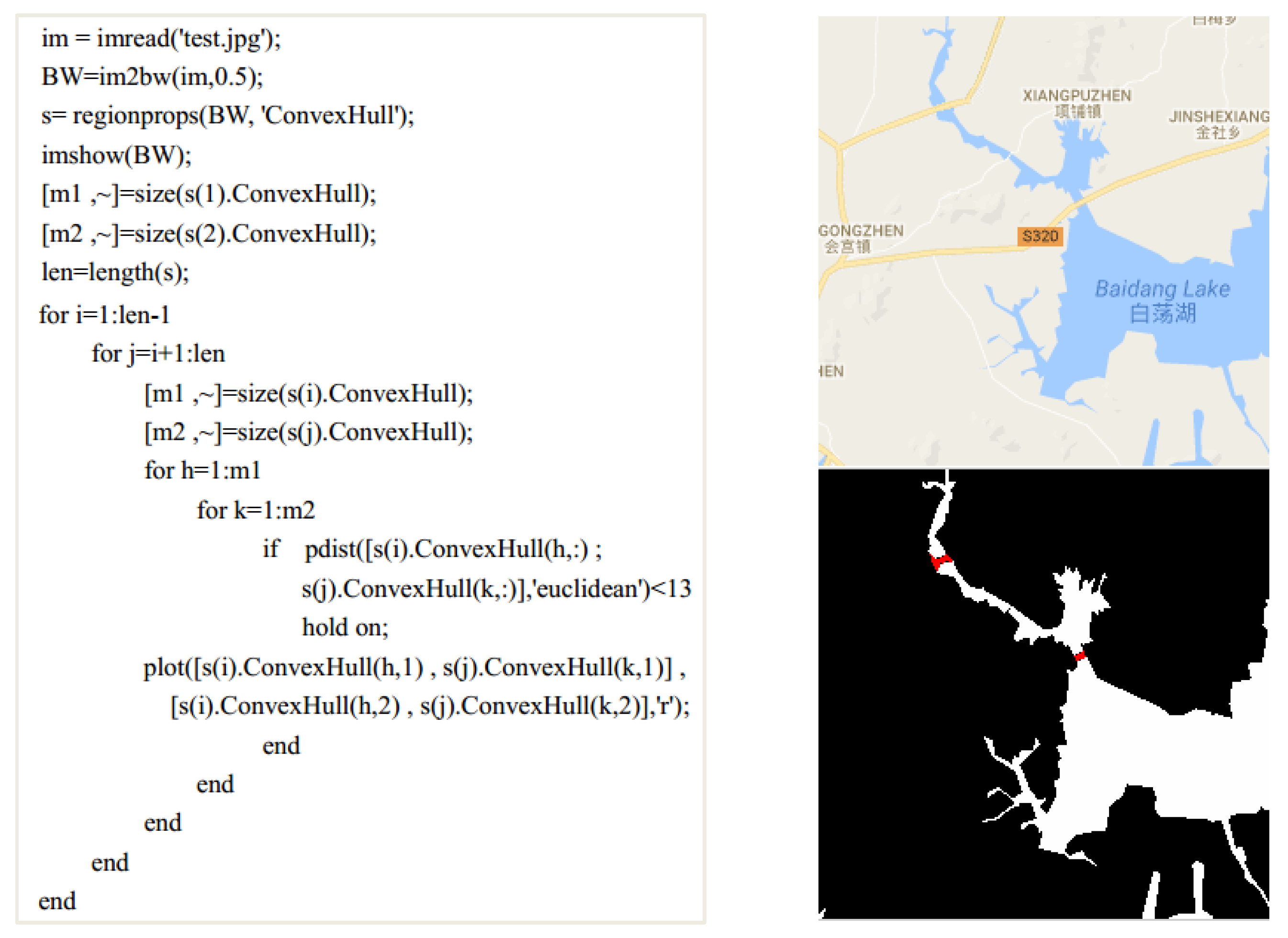
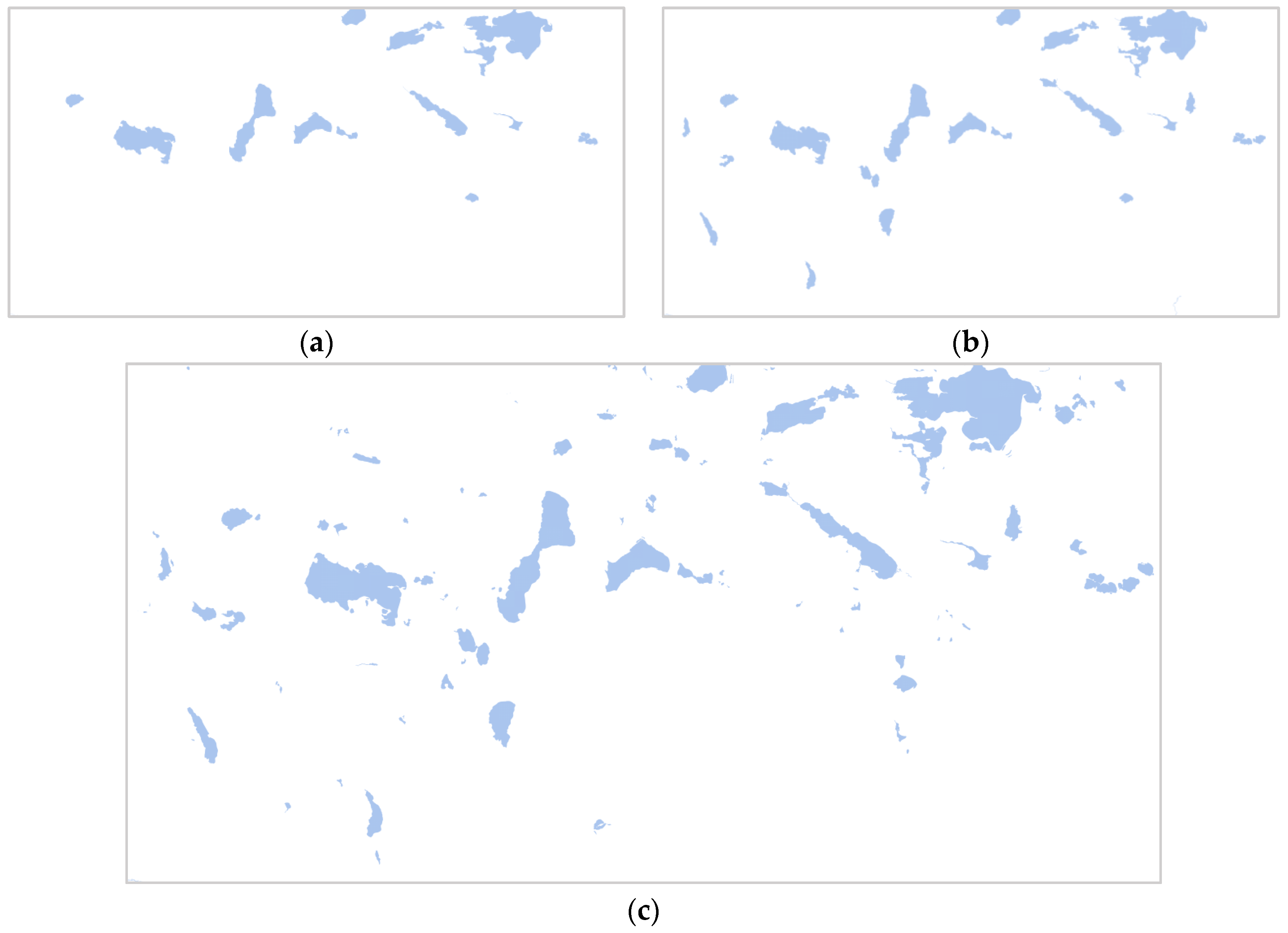
4.1.2. Connection of Fractured Water Areas

The water areas may exhibit fractures because of the overlay relationships between water features and other geographic elements such as roads in the map. As shown in the upper right of Figure 10, the roads, which overlie the river, produce fractures in the extracted river. We use an algorithm that is based on convex hulls to connect these fractures. The pseudo code is shown on the left side of Figure 10, and the results after using the algorithm to connect the fractures are shown on the right. The algorithm adequately maintains the original width and orientation of the river.

4.1.3. Filling Holes in Water Areas

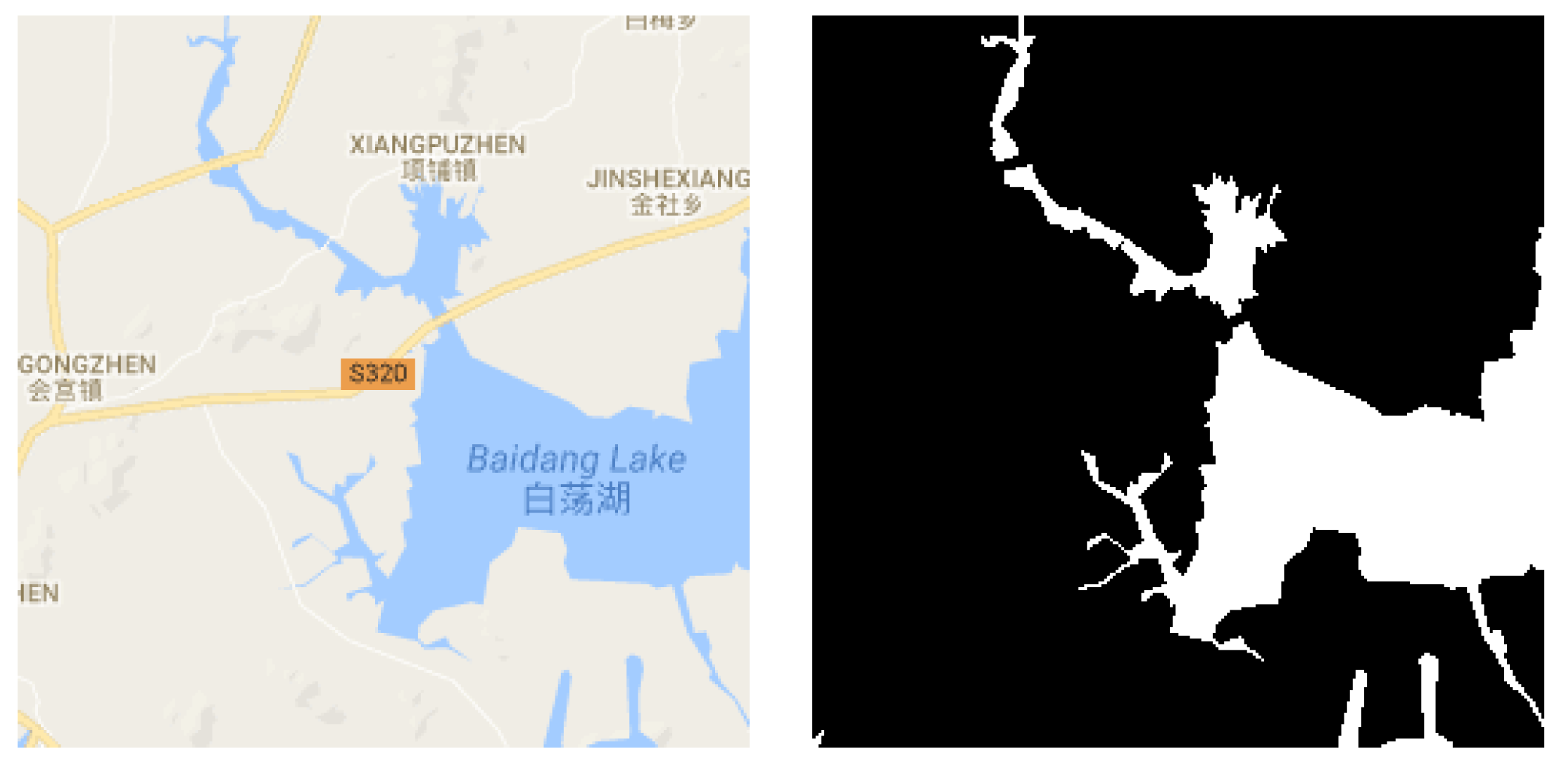
The extraction areas corresponding to some larger water areas contain holes because of the presence of annotations, as shown in the central part of Figure 11. Whether the regions surrounding annotations contain water pixels must be determined to address this problem. When the neighborhoods contain water pixels, the annotation pixels are marked as water pixels. Otherwise, the annotation pixels are not marked. The results that are generated after using this method to fill the holes are shown on the right side of Figure 11.

4.2. Study Area

In this study, experimental data that were used to detect changes in water areas over multiple scales were obtained from the Tiandi map for China. We used data covering the tenth through the twelfth levels from the Tiandi map. The study area is located in the western part of the Autonomous Region of Tibet in China. Several lakes and a few rivers are present within this area. The study area is located between 34.34 and 36.62 degrees north in latitude and between 89.97and 92.87 degrees east in longitude. The data at the tenth level consists of 128 tiles, and the size of one tile is 256 by 256 pixels. As the level increases, the total number of tiles also increases, according to the rules of the pyramid. The data at the highest level, namely the 12th level, include 2048 tiles. The coordinate range of these tiles is $6144\le x\le 6207$, $3200\le y\le 3263$. The image that is formed from these tiles contains 8192 by 16,384 pixels.

Many overlying features such as roads and annotations intersect the lakes. We can use the methods described in Section 4.1 to extract the lakes. Figure 12 shows the results of the extraction for the tenth to twelfth levels. The results after fracture connection and hole filling are satisfactory.

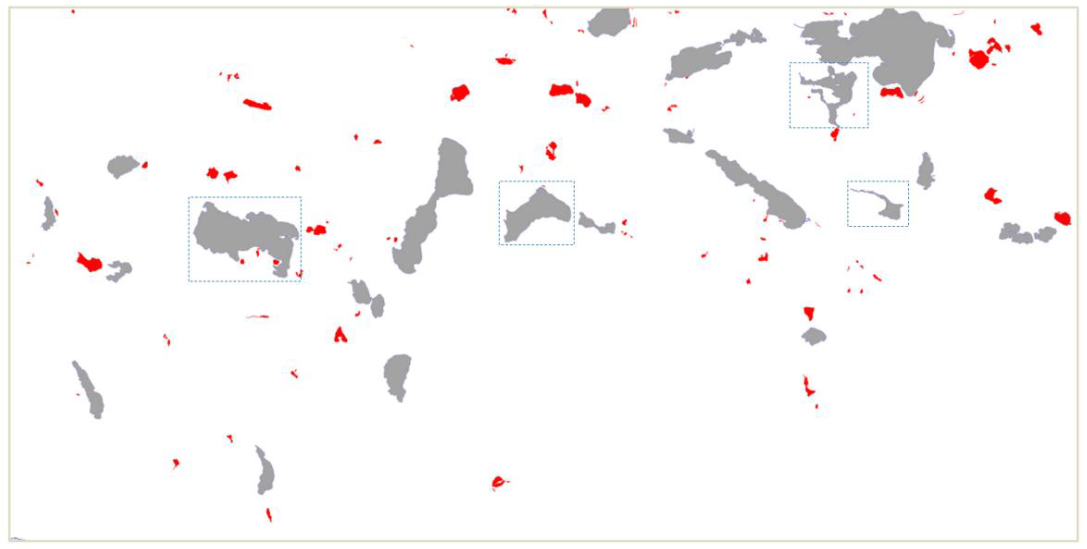
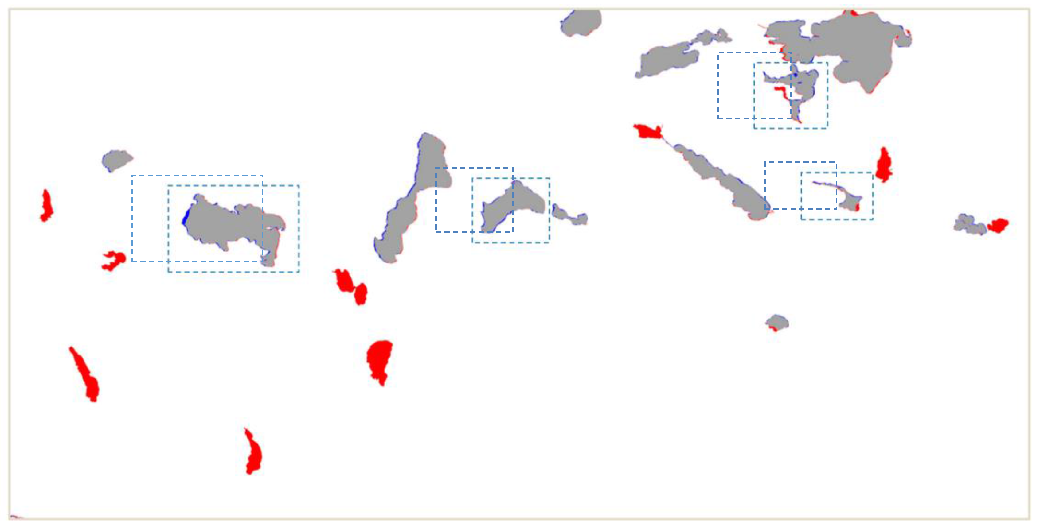
4.3. Results and Analysis

Figure 13 shows the overlapping of the lakes at the tenth and eleventh levels. Figure 14 shows the overlapping of the lakes at the eleventh and twelfth levels. Figure 15 shows the matching results in terms of the local degree of consistency of several typical lakes.

Table 2. Calculation results of the indices.

	Level	Keypoints	Matches	LC	GC	OD	C	Grade
a	10–11	109/212	55/91	0.46	0.9	0.96	0.77	Moderately
	11–12	212/313	155/181	0.65	1	0.99	0.89	Highly
b	10–11	51/106	16 /40	0.35	0.9	0.95	0.74	Less
	11–12	106/140	71 /89	0.65	1	0.99	0.89	Highly
c	10–11	23/60	6/15	0.26	0.9	0.90	0.71	Low
	11–12	60/100	44 /66	0.70	1	0.99	0.91	Exactly
d	10–11	65/205	33 /71	0.43	0.8	0.92	0.70	Less
	11–12	205/301	137/165	0.61	1	0.99	0.88	Highly

shows the calculation results of the global degree of consistency, local degree of consistency, and degree of overlap of these lakes.

As shown in Figure 13 and Figure 14, many regions at levels 10 and 11 do not fully overlap after overlapping the matching lakes, and these non-overlapping regions are marked in red and blue. However, at levels 11 and 12, these non-overlapping regions are relatively less common. We select four typical lakes from all of the lakes within the study area to show the calculation process and the parameters that are used. Four lakes, a, b, c, and d, are shown in Figure 15. Each of these lakes includes four feature matches. The two images on the left are the results of the positive and negative matching of local features at levels 10 and 11, and the two images on the right are the results of the positive and negative matching of local features at levels 11 and 12. The intersecting lines show incorrect matches; however, few incorrect matches are observed, and these features did not notably influence the measurement of the local features. Table 2 shows that the number of local feature points noted in the lakes at levels 11 and 12 was greater than the number of local feature points noted in the lakes at levels 10 and 11. Therefore, the lakes at levels 10 and 11 were moderately or less consistent, whereas the lakes at levels 11 and 12 were exactly or highly consistent.

Figure 16 shows the final results of the consistency assessment between the three levels. The results indicate that the degree of consistency of the lakes at levels 10 and 11 is relatively low, as reflected by the grades associated with the matches (less consistent, moderately consistent, and inconsistent). However, the degree of consistency of the lakes at levels 11 and 12 is relatively high, and the corresponding grades are highly consistent, exactly consistent, and inconsistent. The inconsistent lakes are almost completely new.

Table 3. Detection results.

Grade	Total (10–11)	Percentage (10–11)	Total (11–12)	Percentage (11–12)
Exactly	0	0%	3	2.4%
Highly	0	0%	19	15.0%
Moderately	8	36.4%	0	0%
Less	5	22.7%	0	0%
Inconsistent	9	40.9%	105	82.6%

shows the final number and proportion of the different degrees of consistency. As shown in Table 3, the proportion of inconsistent lakes at levels 10 and 11 is the highest, and these lakes make up 40.9% of all the lakes; the proportion of moderately consistent lakes is the second largest, and these lakes make up 36.4% of all the lakes; and the proportion of less consistent lakes is the lowest, and these lakes make up only 22.7% of all the lakes. At levels 11 to 12, the number of lakes increased significantly and all the consistency grades are highly consistent or exactly consistent, except for those for the added lakes. The exactly consistent lakes make up 2.4% of all the lakes, and the highly consistent lakes make up 15.0% of all the lakes. The proportion of new inconsistent lakes is the highest, and they make up 82.6% of all the lakes.

5. Conclusions

Consistency among spatial objects at different resolutions is a key issue in many scale-dependent applications such as querying spatial data at different resolutions, integrating spatial data from multiple sources, and rapidly transmitting spatial data in a networked environment. Therefore, evaluating, checking, and maintaining the consistency of spatial data at different resolutions is very important. All existing studies use vector data to assess the consistency of objects, whereas consistency that is based on raster data remains an open problem. Moreover, previous study objects were confined to buildings, roads, or land-cover data, but water is also an important component of maps. This paper focused on the consistency of water areas at different scales. In particular, we described a hierarchical approach that uses both global and local image features to measure consistency based on raster tiles. Three types of characteristic indices were proposed to measure the degree of consistency of multiscale representations of water areas. These indices were the degree of global feature consistency, the degree of local feature consistency and the degree of overlap. The degree of consistency of pairs of objects was divided into five grades, specifically exactly consistent, highly consistent, moderately consistent, less consistent, and inconsistent, through the analysis of global and local features. We also extracted independent water areas from a tile map and found that the proposed methods were effective.

As there are many potential types of unreasonable inconsistencies, our study has practical utility in the verification and maintenance of spatial data quality for use in several types of applications: (1) Supporting decision making. In this paper, we have provided metrics for assessing the consistency of multiscale representations of water areas and grading the degree of inconsistency. In the process of removing unreasonable inconsistencies, it will be useful to decide which inconsistencies can be neglected, which inconsistencies are worth noting, and which inconsistencies should receive attention or be corrected (such as those associated with the highly consistent, less consistent, and inconsistent grades, respectively). (2) Checking for updates. When map suppliers update the map data that underlie their services, there is no need to update all the data. Our study can help to distinguish which data must be updated, which data can be updated, and which data do not need to be updated. (3) Data filtering. When users upload data to the map database of a map supplier in a VGI system, our methods can help to filter out inconsistent data and avoid the entering of erroneous data into the database. However, some incorrect matches were obtained when we used the SIFT algorithm to calculate the local characteristics of water areas. The development of more effective and reasonable methods for feature extraction and matching is worthy of further study. In addition, the methods used for measuring the consistency of other geographical elements such as buildings, roads, and annotations should be considered for use with tile maps in the future.

References

1. Goodchild, M.F.; Li, L. Assuring the quality of volunteered geographic information. Spat. Stat. 2012, 1, 110–120. [Google Scholar] [CrossRef]
2. Goodchild, M.F.; Muller, J.C. Issues of Quality and Uncertainty. In Advances in Cartography; Muller, J.-C., Ed.; Elsevier: London, UK, 1991; pp. 113–139. [Google Scholar]
3. Bertolotto, M.; Egenhofer, M.J. Progressive transmission of vector data over the World Wide Web. GeoInformatica 2001, 5, 345–373. [Google Scholar] [CrossRef]
4. Parent, C.; Spaccapietra, S.; Zimanyi, E. The MurMur project: Modeling and querying multi-representation spatio-temporal databases. Inf. Syst. 2006, 5, 733–769. [Google Scholar] [CrossRef]
5. Duckham, M.; Lingham, J.; Mason, K.; Worboys, M. Qualitative reasoning about consistency in geographic information. Inf. Sci. 2006, 176, 601–627. [Google Scholar] [CrossRef]
6. Goodchild, M.F. Citizens as sensors: The world of volunteered geography. GeoJournal 2007, 69, 211–221. [Google Scholar] [CrossRef]
7. Du, H.; Anand, S.; Alechina, N.; Morley, J.; Hart, G.; Leibovici, D.; Jackson, M.; Ware, M. Geospatial information integration for authoritative and crowd sourced road vector data. Trans. GIS 2012, 16, 455–476. [Google Scholar] [CrossRef]
8. Yang, B.; Zhang, Y.; Luan, X. A probabilistic relaxation approach for matching road networks. Int. J. Geogr. Inf. Sci. 2012, 27, 319–338. [Google Scholar] [CrossRef]
9. Koukoletsos, T.; Haklay, M.; Ellul, C. Assessing data completeness of VGI through an automated matching procedure for linear data. Trans. GIS 2012, 16, 477–498. [Google Scholar] [CrossRef]
10. Abdelmoty, A.I.; Jones, C.B. Towards Maintaining Consistency of Spatial Databases. In Proceedings of the Sixth International Conference on Information and Knowledge Management, Las Vegas, NV, USA, 10–14 November 1997; pp. 293–300. [Google Scholar]
11. Dettori, G.; Puppo, E. How Generalization Interacts with the Topological and Metric Structure of Maps. In Proceedings of the 7th International Symposium on Spatial Data Handling, London, UK, 12–16 August 1996; pp. 9–27. [Google Scholar]
12. Delis, V.; Hadzilacos, T. On the Assessment of Generalisation Consistency. In Proceedings of the International Symposium on Advances in Spatial Databases, Berlin, Germany, 15–18 July 1997; pp. 321–335. [Google Scholar]
13. Du, S. Evaluating structural and topological consistency of complex regions with broad boundaries in multi-resolution spatial databases. Inf. Sci. 2008, 178, 52–68. [Google Scholar] [CrossRef]
14. Rodríguez, A. Inconsistency issues in spatial databases. In Inconsistency Tolerance, 1st ed.; Bertossi, L., Hunter, A., Schaub, T., Eds.; Lecture Notes in Computer Science 3300; Springer: Berlin/Heidelberg, Germany, 2005; pp. 237–269. [Google Scholar]
15. Egenhofer, M.J.; Sharma, J. Topological Consistency. In Proceedings of the Fifth International Symposium on Spatial Data Handling, Charleston, SC, USA, 3–7 August 1992; pp. 335–343. [Google Scholar]
16. Tryfona, N.; Egenhofer, M.J. Multi-resolution Spatial Databases: Consistency among Networks. In Proceedings of the Sixth International Workshop on Foundations of Models and Languages for Data and Objects, Schloss Dagstuhl, Germany, 16–20 September 1996; pp. 119–132. [Google Scholar]
17. Tryfona, N.; Egenhofer, M.J. Consistency among parts and aggregates: A computational model. Trans. GIS 1996, 1, 189–206. [Google Scholar] [CrossRef]
18. Kang, H.K.; Kim, T.W.; Li, K.J. Topological Consistency for Collapse Operation in Multiscale Databases. In Proceedings of the 23rd International Conference on Conceptual Modeling, Berlin, Germany, 8–12 November 2004; pp. 91–102. [Google Scholar]
19. Du, S.; Guo, L.; Wang, Q. A scale-explicit model for checking directional consistency in multiresolution spatial data. Int. J. Geogr. Inf. Sci. 2010, 24, 465–485. [Google Scholar] [CrossRef]
20. Rodríguez, M.A.; Brisaboa, N.; Meza, J.; Luaces, M.R. Measuring Consistency with Respect to Topological Dependency Constraints. In Proceedings of the 18th SIGSPATIAL International Conference on Advances in Geographic Information Systems, San Jose, CA, USA, 2–5 November 2010; pp. 182–191. [Google Scholar]
21. Brisaboa, N.R.; Luaces, M.R.; Andrea Rodríguez, M.; Seco, D. An inconsistency measure of spatial data sets with respect to topological constraints. Int. J. Geogr. Inf. Sci. 2014, 28, 56–82. [Google Scholar] [CrossRef]
22. Ang, Y.H.; Li, Z.; Ong, S.H. Image Retrieval based on Multidimensional Feature Properties. In Proceedings of the Symposium on Electronic Imaging: Science & Technology, San Jose, CA, USA, 23 March 1995; pp. 47–57. [Google Scholar]
23. Zahn, C.T.; Roskies, R.Z. Fourier descriptors for plane closed curves. IEEE Trans. Comput. 1972, 100, 269–281. [Google Scholar] [CrossRef]
24. Veltkamp, R.C. Shape Matching: Similarity Measures and Algorithms. In Proceedings of the SMI 2001 International Conference on Shape Modeling and Applications, San Jose, CA, USA, 7–11 May 2001; pp. 188–197. [Google Scholar]
25. Lee, D.J.; Antani, S.; Long, L.R. Similarity Measurement Using Polygon Curve Representation and Fourier Descriptors for Shape-based Vertebral Image Retrieval. In Proceedings of the SPIE on Medical Imaging 2003: International Society for Optics and Photonics, San Diego, CA, USA, 16 May 2003; pp. 1283–1291. [Google Scholar]
26. Mortara, M.; Spagnuolo, M. Similarity measures for blending polygonal shapes. Comput. Graph. 2001, 25, 13–27. [Google Scholar] [CrossRef]
27. Latecki, L.J.; Lakamper, R. Shape similarity measure based on correspondence of visual parts. IEEE Trans. Pattern Anal. Mach. Intell. 2000, 22, 1185–1190. [Google Scholar] [CrossRef]
28. McMaster, R.B.; Shea, K.S. Generalization in Digital Cartography; Association of American Geographers: Washington, DC, USA, 1992. [Google Scholar]
29. Goodchild, M.; Jeansoulin, R. Data Quality in Geographic Information: From Error to Uncertainty, 1st ed.; Hermes: Paris, France, 1998. [Google Scholar]
30. Egenhofer, M.J.; Clemeentini, E.; Felice, P.D. Evaluating inconsistencies among multiple representations. In Proceedings of the 6th International Symposium on Spatial Data Handling, Edinburgh, UK, 5–9 September 1994; pp. 901–920. [Google Scholar]
31. Sheeren, D.; Mustière, S.; Zucker, J.D. Consistency Assessment between Multiple Representations of Geographical Databases: A Specification-based Approach. In Developments in Spatial Data Handling, 1st ed.; Springer: Berlin/Heidelberg, Germany, 2005; pp. 617–628. [Google Scholar]
32. Ai, T.; Ke, S.; Yang, M.; Li, J. Envelope generation and simplification of polylines using Delaunay triangulation. Int. J. Geogr. Inf. Sci. 2017, 31, 297–319. [Google Scholar] [CrossRef]
33. Ai, T.; Li, J. A DEM generalization by minor valley branch detection and grid filling. ISPRS J. Photogramm. Rem. Sens. 2010, 65, 198–207. [Google Scholar] [CrossRef]
34. Müler, J.C.; Zeshen, W. Area-patch generalisation: A competitive approach. Cartogr. J. 1992, 29, 137–144. [Google Scholar] [CrossRef]
35. Sheeren, D.; Mustière, S.; Zucker, J.D. A data-mining approach for assessing consistency between multiple representations in spatial databases. Int. J. Geogr. Inf. Sci. 2009, 23, 961–992. [Google Scholar] [CrossRef]
36. Schneider, M.; Chang, S.F. A Robust Content Based Digital Signature for Image Authentication. In Proceedings of the 3rd IEEE International Conference on Image Processing, Lausanne, Switzerland, 19 September 1996; pp. 227–230. [Google Scholar]
37. Swaminathan, A.; Mao, Y.; Wu, M. Robust and secure image hashing. IEEE Trans. Inf. Forensics Secur. 2006, 1, 215–230. [Google Scholar] [CrossRef]
38. Li, Y.; Lu, Z.; Zhu, C.; Niu, X. Robust image hashing based on random gabor filtering and dithered lattice vector quantization. IEEE Trans. Image Process. 2012, 21, 1963–1980. [Google Scholar] [PubMed]
39. Zhao, Y.; Wang, S.; Zhang, X.; Yao, H. Robust hashing for image authentication using zernike moments and local features. IEEE Trans. Inf. Forensics Secur. 2013, 8, 55–63. [Google Scholar] [CrossRef]
40. Lowe, D.G. Object Recognition from Local Scale-Invariant Features. In Proceedings of the Seventh IEEE International Conference on Computer Vision, Kerkyra, Greece, 20–27 September 1999; pp. 1150–1157. [Google Scholar]
41. Lowe, D.G. Distinctive image features from scale-invariant keypoints. Int. J. Comput. Vis. 2004, 60, 91–110. [Google Scholar] [CrossRef]
Figure 1. Inconsistencies between lakes at different scales.
Ijgi 06 00240 g001
Figure 2. Feature comparison at the global and local levels.
Ijgi 06 00240 g002
Figure 3. Framework for measuring consistency.
Ijgi 06 00240 g003
Figure 4. Tile-map pyramid.
Ijgi 06 00240 g004
Figure 5. Global feature calculation. (a) Determine the calculation region; (b) Grayscale image.
Ijgi 06 00240 g005
Figure 6. Local feature calculation using the scale-invariant feature transform (SIFT) algorithm. (a) A lake from a low level; (b) The same lake from a high level; (c) Matching results.
Ijgi 06 00240 g006
Figure 7. Degree of overlap.
Ijgi 06 00240 g007
Figure 8. Typical examples of consistency divisions. (a) G C = 1 , L C = 0.53 , O D = 0.99 , and C = 0.86 . Grade: highly consistent; (b) G C = 1 , L C = 0.50 , O D = 0.99 , and C = 0.85 . Grade: highly consistent; (c) G C = 0.9 , L C = 0.34 , O D = 0.96 , and C = 0.74 . Grade: less consistent; (d) G C = 0.4 , L C = 0.33 , O D = 0.85 , and C = 0.42 . Grade: inconsistent; (e) G C = 1 , L C = 0.68 , O D = 0.75 , and C = 0.88 . Grade: highly consistent.
Ijgi 06 00240 g008
Figure 9. Extracted water areas with colour segmentation.
Ijgi 06 00240 g009
Figure 10. Water-area fracture connection.
Ijgi 06 00240 g010
Figure 11. Water-area hole filling.
Ijgi 06 00240 g011
Figure 12. Experimental data after extraction. (a) Tenth level; (b) Eleventh level; (c) Twelfth level.
Ijgi 06 00240 g012
Figure 13. Overlay of the tenth and eleventh levels.
Ijgi 06 00240 g013
Figure 14. Overlay of the eleventh and twelfth levels.
Ijgi 06 00240 g014
Figure 15. Matching results. (a) Level 10–11: L C = 0.46 , level 11–12: L C = 0.65 ; (b) Level 10–11: L C = 0.35 , level 11–12: L C = 0.65 ; (c) Level 10–11: L C = 0.26 , level 11–12: L C = 0.70 ; (d) Level 10–11: L C = 0.43 , level 11–12: L C = 0.61 .
Ijgi 06 00240 g015
Figure 16. Detection results.
Ijgi 06 00240 g016aIjgi 06 00240 g016b