Article

Monitoring and Modeling of Spatiotemporal Urban Expansion and Land-Use/Land-Cover Change Using Integrated Markov Chain Cellular Automata Model

1
The State Key Laboratory of Remote Sensing Science, Institute of Remote Sensing and Digital Earth, Chinese Academy of Sciences, Beijing 100101, China
2
Institutes of Ecology, Friedrich Schiller University, Jena 07743, Germany
3
College of Natural Resources, University of Tehran, Tehran 1417466191, Iran
4
Institute of Remote Sensing and GIS, School of Earth and Space Science, Peking University, Beijing 100871, China
*
Author to whom correspondence should be addressed.
ISPRS Int. J. Geo-Inf. 2017, 6(9), 288; https://doi.org/10.3390/ijgi6090288
Submission received: 7 August 2017 / Revised: 1 September 2017 / Accepted: 6 September 2017 / Published: 8 September 2017

Abstract

:
Spatial–temporal analysis of land-use/land-cover (LULC) change as well as the monitoring and modeling of urban expansion are essential for the planning and management of urban environments. Such environments reflect the economic conditions and quality of life of the individual country. Urbanization is generally influenced by national laws, plans and policies and by power, politics and poor governance in many less-developed countries. Remote sensing tools play a vital role in monitoring LULC change and measuring the rate of urbanization at both the local and global levels. The current study evaluated the LULC changes and urban expansion of Jhapa district of Nepal. The spatial–temporal dynamics of LULC were identified using six time-series atmospherically-corrected surface reflectance Landsat images from 1989 to 2016. A hybrid cellular automata Markov chain (CA–Markov) model was used to simulate future urbanization by 2026 and 2036. The analysis shows that the urban area has increased markedly and is expected to continue to grow rapidly in the future, whereas the area for agriculture has decreased. Meanwhile, forest and shrub areas have remained almost constant. Seasonal rainfall and flooding routinely cause predictable transformation of sand, water bodies and cultivated land from one type to another. The results suggest that the use of Landsat time-series archive images and the CA–Markov model are the best options for long-term spatiotemporal analysis and achieving an acceptable level of prediction accuracy. Furthermore, understanding the relationship between the spatiotemporal dynamics of urbanization and LULC change and simulating future landscape change is essential, as they are closely interlinked. These scientific findings of past, present and future land-cover scenarios of the study area will assist planners/decision-makers to formulate sustainable urban development and environmental protection plans and will remain a scientific asset for future generations.

1. Introduction

Policy makers in developing countries face unprecedented challenges with regard to governing, urban planning and land-use/land-cover (LULC) management because of the prevailing high dynamic growth. Therefore, knowledge concerning past, current and future growth plays an important role in the decision-making process [1]. The conversion of natural habitats into agricultural land for the maintenance of human livelihoods has been identified as the greatest driver of global environment change [2]. The spatial distribution of agricultural land for urban development [3,4,5] and heterogeneous settlement patterns over agricultural land is a universal trend [6]. Changes in LULC and rapid urban growth are subjects of great concern worldwide. Rural–urban migration, natural population growth and administrative reclassification of rural areas to urban areas are the major components [7,8] of global patterns of urbanization [9,10]. World population crossed the first billion mark in 1830, reached 2 billion in 1930, 3 billion in 1960, 5 billion in 1987, 6 billion in 1999 [11], 7.6 billion in 2017 and is projected to reach 8.6 billion in 2030, 9.8 billion in 2050 and 11.2 billion in 2100 [12]. The world urban population has increased much faster than with rural population and it was 14% in 1900 to 29.1% in 1950, 47% in 2005 [11] and 2014 accounted for 54% and projected about 66% by 2050 [13]. As a result of various anthropogenic and natural factors, developing countries experience relatively more rapid urban growth and LULC changes than developed countries [14] and this growth triggers several environmental and ecological problems at multiple spatial scales [1,14,15,16,17].
In recent decades, Southeast Asia and other developing countries under transitional economies (e.g., Cambodia, Laos, Myanmar and Vietnam) [18] as well as their cities have recorded a higher rate of urbanization [14]. There was an increase in urban population from 9%, 12%, 24% and 19% in 1980 to 20%, 32%, 33% and 35% in 2012 regarding Cambodia, Laos, Myanmar and Vietnam, respectively [18]. Despite its short urban history, Nepal has recorded the highest urban growth rate (6.6%) in South Asia exceeding Sri Lanka (2.2%), India (2.9%), Pakistan (4.4%) and Bangladesh (5.3%) [19]. In the last 50 years, Nepal’s population has increased nearly threefold, but the area of cultivated land has only increased twofold during the same period [20]. The urban population of Nepal was 2.9% in 1952/54 and increased to 40.49% in 2015 [21]. Such trend of urban expansion is a serious issue for sustainable urban development in developing countries [22]; since it is directly associated with sustainability issues such as food security and a secured urban future.
Remote sensing and a geographical information system (GIS) have been applied extensively to help understand the spatiotemporal patterns of urbanization [11] and urban planning [23]. They have proven to be significant, powerful [16,17], cost effective and accurate [14,18,24,25]. Different simulation and empirical models have been applied to predict changes in LULC [26,27]; however, few have used system dynamics models to determine the main drivers [28]. Spatial simulation models are efficient tools for quantitative simulation [29] and integrating the Markov-chain model and cellular automata (CA) is considered by some to be one of the best options for the analysis of LULC on different spatial scales [30]. One of the basic assumptions of the Markov chain LULC change is a stochastic process which describes the probability of one state i changing to another state j [25,29,31]. The CA model predicts spatial change over a specific time period using a probability matrix [29].
Economic growth is indicated by the occurrence of urban sprawl and population growth. However, human-induced deforestation and development of the natural landscape to establish building, water supply, sewage, transport networks and large scale of construction work create multiple unused impacts on land and soil, biodiversity, air, water qualities as well as other environmental activities. Similarly, major construction works transform cities into impervious surfaces with the formation of heat islands which contribute to climate changes including increased occurrences of multiple natural disasters [32,33,34,35].
Thus, it is very important to access, monitor and model past, present and future LULC scenarios using RS/GIS tools and simulation models. This is because obtaining overtime spatial–temporal characteristics is a fundamental prerequisite for the formulation of effective urban policies, as well as economic, demographic and environmental plans to ensure sustainable development and maintain environmental equilibrium [1,13,30,36,37].
The study area of this work is the Jhapa District of Nepal, located in the southern plain of the country. This area has been experiencing accelerated urban growth since 1996. The urbanization process is influenced by migration and population growth has recorded a remarkable impact on other LULC, mostly prime agricultural land. Settlements are scattered and unmanaged and are likely to influence the natural/social environment, thereby resulting in an unbalanced ecosystem. Urban planning and management has been affected due to the lack of reliable urban databases, spatiotemporal information of LULC change and environmental concerns. There exist poor planning, weak institutional capacity and insufficient investment in the urban sector which hinder effective remedies which address urban poverty, disaster risk as well as social and natural environment issues [3,5,6,14,22]. The sustainable development and urban future of the study area is skeptical.
The major objective of this study was to explore the spatiotemporal analysis of LULC, monitor past/present urban expansion trends and future change simulation by 2026 and 2036, using the CA–Markov Model. More specific objectives are to (a) analyze the spatiotemporal dynamics of LULC from 1989 to 2016, (b) evaluate the urban expansion ratio and spatiotemporal extent, and (c) predict future LULC change by 2026 and 2036.

2. Materials and Methodology
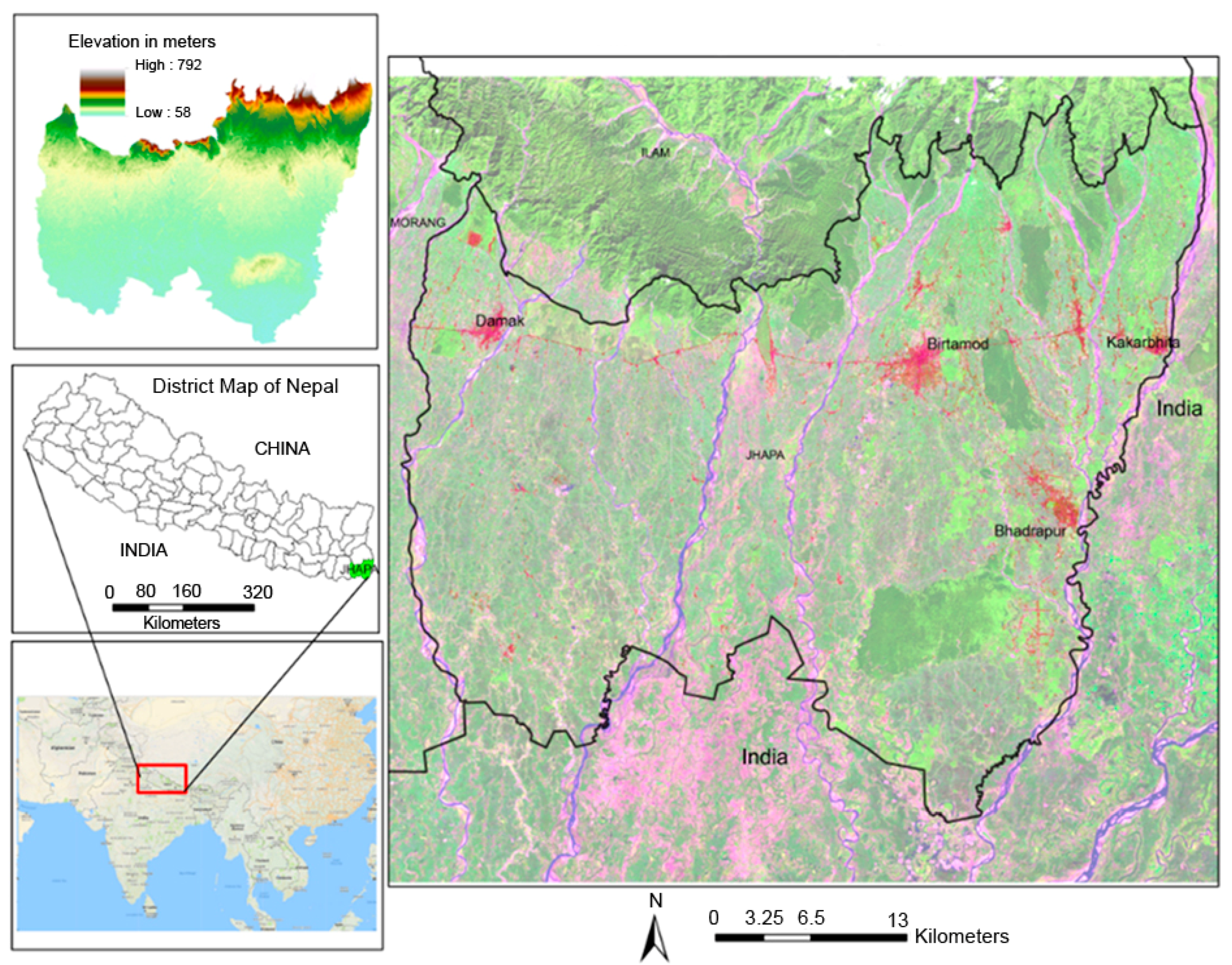
2.1. Study Area

The study area, Jhapa district is located between 26.36°, 26.80°, 87.63° and 88.20° in the southern part of Nepal (Figure 1). The district shares its eastern and southern boundaries with India and its northern and western boundaries with Ilam and Morang districts, respectively. Administratively, it is divided into eight municipalities and seven rural municipalites. There was an increase in the district population from 593,737 in 1991 to 688,109 in 2001 and 812,650 in 2011 [20].
Jhapa district has a subtropical monsoon climate with summer temperatures ranging from 32 to 35 °C, winter temperatures ranging from 8 to 15 °C and an average annual rainfall of 270 mm. It is low lying, at 58 to 792 m in elevation and has highly fertile soil where rice, wheat, maize, oilseed, pulses, and cash crops such as tea, jute and nuts are grown. The area is rich in biodiversity, containing subtropical evergreen hardwood forests to decideous forests depending on the altitude [38]. Geologically, the area has sediment of the Indo-Gangetic plain, rocks from the Siwalik range as well as small parts of the Lesser Himalaya. The Himalayan frontal thrust, Intra Chure thrust and main boundary thrust are located in the southern to northern parts. The Mechi, Deuniya, Biring, Kankai, Ratuwa and Mawa Khola are major rivers experiencing bankfull discharges during the monsoon season, resulting in river bank erosion and loss of farmland. The district is well supplied with water and has a good climate that makes it a major agricultural center. Several proximate and underlying causes are contributing to the migration of people to the area and have increased the population density in the district and urbanization, often at the expense of prime agricultural land.

2.2. Satellite Data and Pre-Processing

For spatial–temporal analysis of LULC change and monitoring of urban expansion of the study area, six time-series of atmospherically-corrected surface reflectance Landsat images from 1989 to 2016 were obtained from the United States Geological Survey (USGS) website [39]. All scenes were verified for geometric accuracy and all data were projected on WGS 1984, UTM zone 45N. Surface reflectance data are ready for application and these data sets have been post-production processed and included atmospheric correction, geometric correction as well as other adjustments (for more details visit: http://landsat.usgs.gov/CDR_LSR.php). The maximum cloud-free images were included in the study. All scenes were verified for geometric accuracy and all data was projected on to UTM WGS 1984, zone 45N. Overall, the OLI bands are spectrally narrower than the ETM+ band, particularly in the near infrared (NIR) region [40,41]. The ultra-blue band (0.43–0.451 μm) of Landsat 8 was removed for consistency and renamed for other images (e.g., 1, 2, 3, 4, 5 and 7). Band 1 of Landsat 8 was used for the coastal areas and shallow water and aerosol, dust and smoke detection studies [40]. For land-cover classification, six images dated 4 December 1989 (Landsat 5), 23 December 1996 (Landsat 5), 29 December 2001 (Landsat 7), 19 December 2006 (Landsat 5), 31 January 2011 (Landsat 5) and 13 January 2016 (Landsat 8) with path/row 139/42 were sampled.
High spatial resolution images from Google Earth [42] and digital topographical maps (scale 1:25,000) published by the Survey Department of the Government of Nepal in 1995 (sheet numbers: 2687 (04D, 07B, 07D, 08A-08D, 11B, 12A, 12B, 12D) and 2688 (01C, 01D, 05A, 05D, 09A, 09C)) [43] were used to validate the results. Region of interest (ROI) boundaries representing district, municipal and village level study areas were delineated for analysis. The Jhapa district profile [38] was also collected for refinement of the study.

2.3. Extraction of LULC Maps and Analysis

Images were stacked, subset and analyzed in the ENVI [44] environment and classified using the maximum likelihood algorithm and change analysis for 1989, 1996, 2001, 2006, 2011 and 2016. Supervised approaches using a maximum likelihood classifier algorithm [23,30,45,46,47,48] were applied for the extraction of LULC. A modified land-cover classification system was used for remote sensing data as recommended by Anderson et al. [49]. For the extraction of LULC, seven classes were identified: urban (built-up), cultivated land, forest, shrub, sand, water bodies and tea farming area (Table 1). The study primarily concentrated on mapping of urban growth and sprawl. Because Jhapa is one of the few important districts for tea farming, this land use has been classified separately. The land change modeler (LCM) of TerrSet software [50] was used to assess changes and transitions in LULC in different years. Assessment of classification accuracy is necessary when LULC maps are derived from remote sensing techniques [24]. Although the accuracy is limited by satellite image resolution [6], accuracy assessment of LULC maps was achieved using a random sampling method. After land-cover classification, 210 sample points were randomly selected for the evaluation of classification accuracy for seven land-cover classes. Accuracy assessment was based on the calculation of the overall accuracy, user’s accuracy, and producer’s accuracy. Due to the unavailability of updated land-cover data, topographical maps (scale 1:25,000) of 1995, field experience and Google Earth images were used as supporting details for accuracy assessment.

2.4. Quantification of LULC Based Transition Analysis

Land-cover change was calculated for six time periods (1989 to 1996, 1996 to 2001, 2001 to 2006, 2006 to 2011 and 2011 to 2016). For each time period, the transition matrix consists of rows and columns of landscape categories at times T1 and T2.

2.5. Measuring Urban Expansion Rate and Analysis of Urban Extent

The urban expansion growth rate [51] of the study area was measured by calculating the total new urban area. The urban expansion rate indicates the average annual urban area growth in succeeding years.
MUER = ( U 2 U 1 ) / ( T 2 T 1 ) × 100
where MUER refers to the urban expansion rate (km2/year) and U1, U2 represent the urban area (km2) between times T1 and T2 in years.
We quantified the centrality of the land-use spatial pattern using the ring-based analysis approach. Ring-based buffer analysis [10,52,53,54,55] was used to explore the urban expansion characteristics based on landscape orientation. The boundary of the buffer zone outward from the city center (Birtamod) was drawn in Arc GIS 10.1 at equal intervals of 2 km. The buffered area from 1989 to 2016 was mapped.

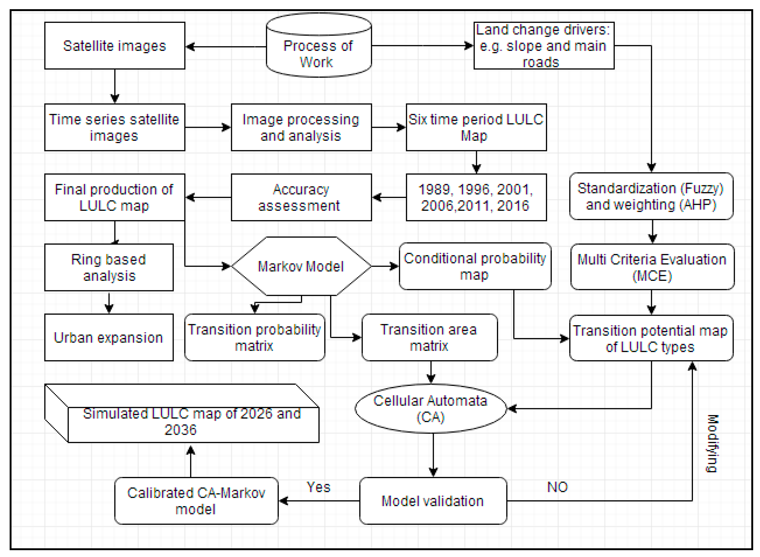
2.6. Simulation of LULC Change

Modeling systems are intended to simplify the complexity of urban systems and make them easier to understand [56]. Markov chain models have been widely applied for ecological modeling [57] as they show the descriptive power and simple trend projection [30]. The CA model addresses spatial allocation and location of change [1] and as it has many advantages for modeling urban phenomena [36] including (a) cell (b) neighborhood, (c) rules, (d) time, and (e) state [29,58,59]. Mainly the modeling system consisted of the following procedures: (a) land-cover maps of 1996, 2006 and 2016 were assessed, (b) the transition area matrix was calculated using the Markov process, (c) transition suitability images were prepared using multi-criteria evaluation (MCE), analytic hierarchy process (AHP) models and fuzzy membership functions in TerrSet and applied in CA–Markov (d) the actual and predicted maps of the year 2016 were evaluated, and finally (e) the LULC maps for the year 2026 and 2036 were simulated using the CA–Markov Model.

2.6.1. CA–Markov Modeling

The Markov model itself does not provide the spatial location of future LULC, so the hybrid CA–Markov was used to achieve the objectives. First, the transition matrix file was created and applied to the model for the specified time of 20 years. Next, CA filters were determined as a standard 5 × 5 contiguity filter in the modeling process. The filter used analysis is based on:
00100
01110
11111
01110
00100
The LULC map of 2016 was used as the base map to simulate LULC maps for the years 2026 and 2036 by calculating the transition area matrix of 2006–2016 and 1996–2016, respectively.

2.6.2. Generating Transition Potential Maps

In this study, GIS algorithms, MCE and fuzzy membership function were applied to extract the transition potential maps of land-cover types. This step determined the status of change. Transition potential maps represent the ability of a pixel to change to a new category or remain unchanged in each transition based on driving factors [60]. In this study, slope, distance to main roads, distance to water bodies and distance to built-up areas were set as driving factors. They were chosen based on their use in similar previous studies [1,29,60]. Fuzzy membership functions (e.g., J-shaped monotonic decrease functions) were used to rescale driver maps into the 0–255 range. AHP was then run to determine the weight of the driving factors using pairwise evaluation. The weighting parameters and control points for each driving factor were chosen based on expert knowledge, interviews and recent similar studies e.g., [1,29,61]. The individual weights and control points determined are listed in Table 2.

2.6.3. Evaluation of Land-Cover Modeling

Evaluation of the model was done by comparing the predicted map for 2016 with the real map of 2016 based on the kappa variation. An accuracy higher than 80% infers some confidence in the simulation [29,61]. A study framework was presented to achieve the research objectives presented in Figure 2.

3. Results and Discussion
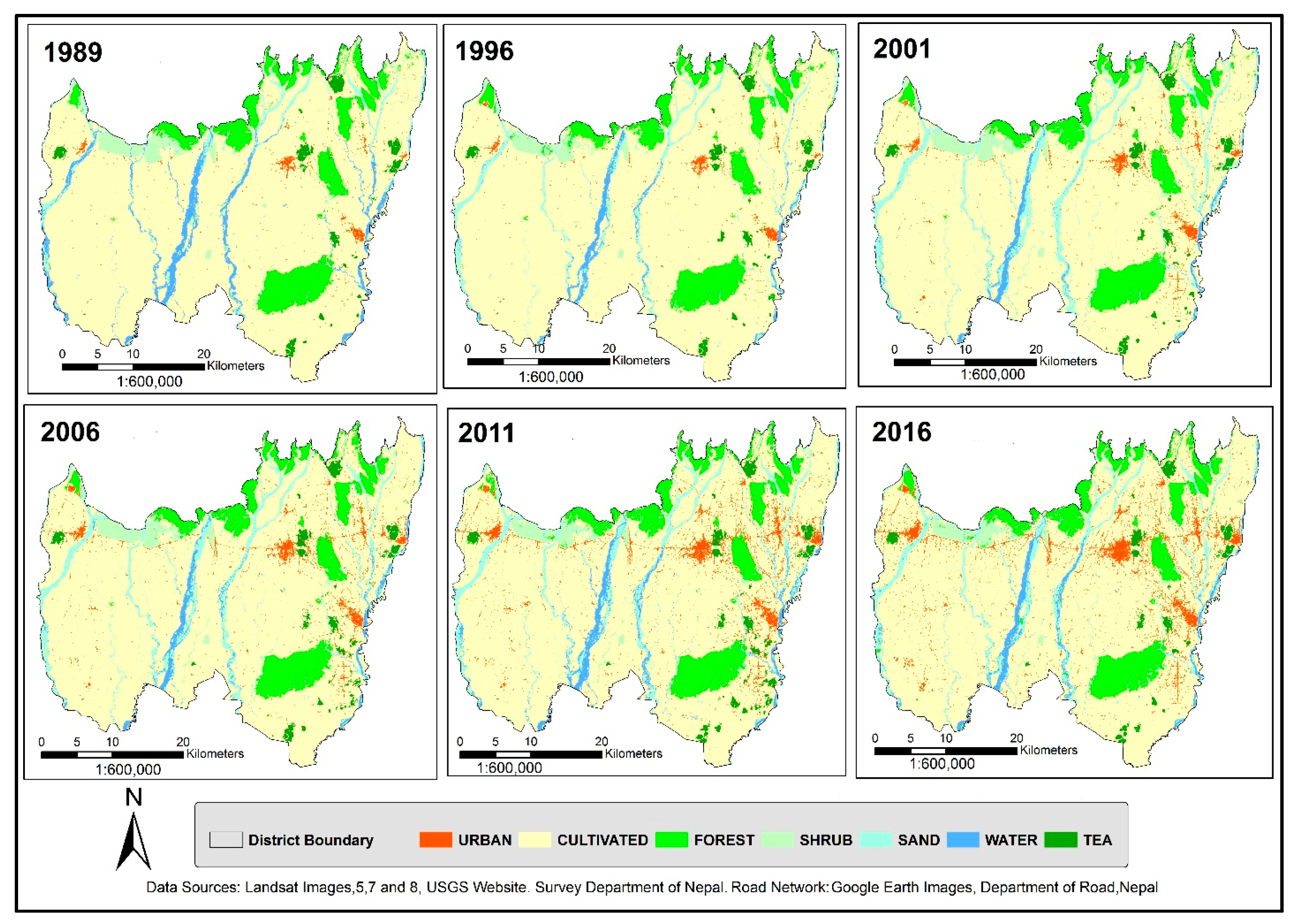
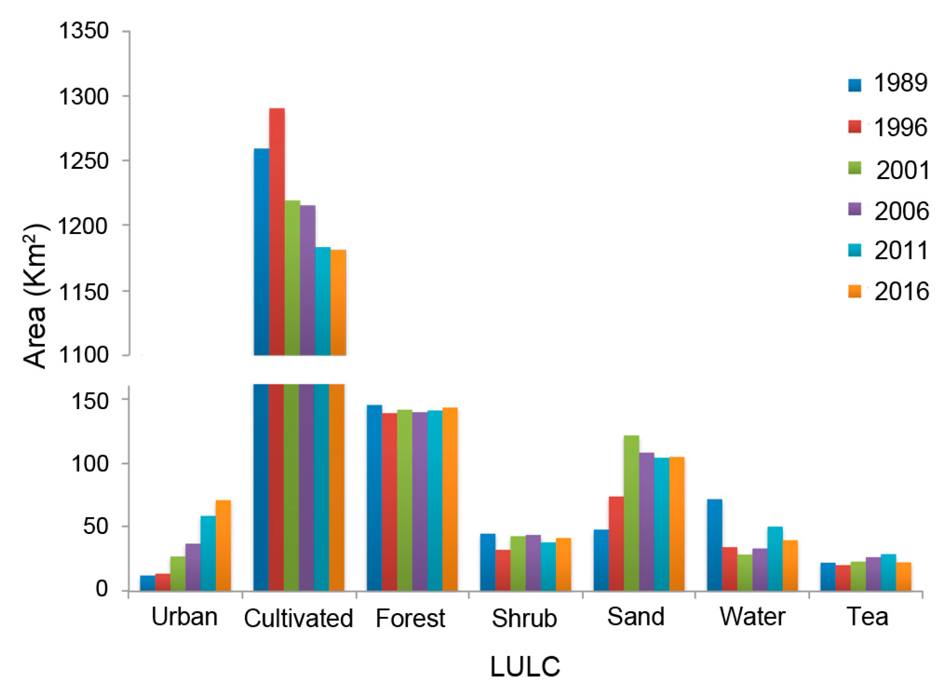
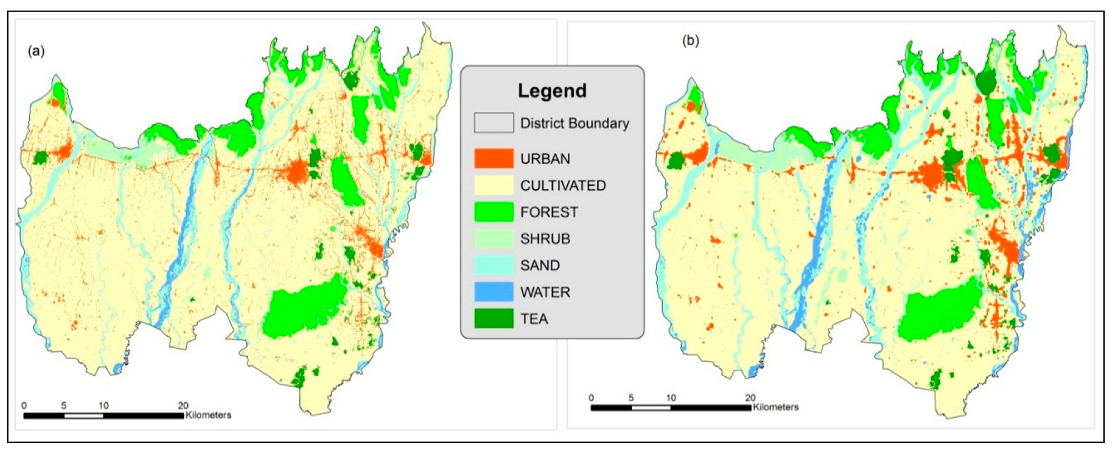
3.1. LULC Dynamics

The overall classification accuracy for the extracted LULC maps were: 1989 (80.66%), 1996 (85.2%), 2001 (82.33%), 2006 (85.88%), 2011 (84.8%) and 2016 (86.2%). These results indicate the suitability of the classified remote sensing images for effective and reliable LULC change analysis and modeling. Also, analysis of user’s and producer’s accuracies shows that the classes with the highest producer’s accuracy were those of tea (100%, 2001), water (96.43%, 2011), and built-up areas (96.31%, 2001) followed by forest (95.59%, 2006). The lowest producer’s accuracy was obtained for sand (76.67%, 2001). User’s accuracy was higher for forest (93.44%, 2016), cultivated lands (93.33%, 1996), and built-up areas (92.53%, 2016), followed by water bodies (91.00%, 1996). The lowest user’s accuracy was found for the sand (73.33%, 1989) (Table 3).
Between 1989 and 2016, a wide range of change in land-use was observed, including a linear increase in urban area, the continuous decline of cultivated land, minimal change in forest cover and shrubs and non-linear transformations of water bodies and sand. The smallest fluctuations were observed for the area of tea farming. Although the water bodies decreased in some time periods, there was no overall decline of permanent water resources. Instead, the area covered by water was seasonal and determined by the changes in rainfall. The Biring, Kankai, Mechi, Deuniya and Ratuwa rivers as well as some streams which cross the district all originate in the mid-hills. The silty Churiya hill is located in the northern belt and during the monsoon season, the swollen rivers spill over causing bank erosion, erosion of agricultural land and accumulation of sand and silt. All these natural activities result in a strongly unpredictable arrangement of sand, water bodies and cultivated land in areas affected by floods.
The study period showed an overall seven-fold increase in urban area for Jhapa district with an area of 12.35 km2 in 1989 increasing to 13.70 km2 in 1996, 27.12 km2 in 2001, 37.09 km2 in 2006, 58.65 km2 in 2011 and 70.90 km2 in 2016. The Central Bureau of Statistics (CBS) 2014 report [25] states that Jhapa is a Tarai district that experienced over 25% inter-district lifetime migration, a high rate of immigration (24.5%) and a low rate of emigration (9.2%). The population density of the district was 299 people per km2 in 1981, which reached 506 per km2 in 2011, for which the national level population density was 180 in 2011. All these factors influenced the population growth of the district. The enormous mass migration, mainly from the adjacent mid-hill districts of Taplejung, Ilam and Panchthar along with the Terhathum and Dhankuta districts was due to political upheaval between 1996 and 2006. After 2006, as the political insurgency settled down, the pace of infrastructure development such as construction of road networks, hospitals, bus parks and academic institutions accelerated. This condition resembles to the urban scenario of Sri Lanka, particularly the Colombo metropolitan area where the development activities were accelerated after the settlement of three decades of civil war in 2009 [62].
The area of cultivated land increased from 1259.34 km2 in 1989 to 1290.34 km2 in 1996 at the cost of shrubs, forest, water, sand and tea (Table 4 and Table 5; Figure 3 and Figure 4). Significant decreases in forest and shrub cover were the other main changes from 1989 to 1996. The shrub area increased from 32.31 to 42.88 km2 and forest cover from 138.57 to 141.23 km2 from 1996 to 2001. Cultivated land experienced a decrease from 1219.26 km2 in 2001 to 1215.43 km2 in 2006 to 1183.34 km2 in 2011 to 1181.26 km2 in 2016. Overall, cultivated land decreased by 78.07 km2 while urban area increased by 58.56 km2 from 1989 to 2016. The region consists of the plain arable land which is strongly affected by floods, especially during monsoon season. Most of the sandy area along the riverbanks in the district has been transformed to cultivated land, which has led the statistical increase in cultivated land; however, fertile agricultural land was converted into urban land.
The tea farming area of 22.25 km2 area in 1989 had decreased to 20.38 km2 by 1996; however, it expanded to 23.10 km2 in 2001, 26.58 km2 in 2006 and 28.95 km2 in 2011 before experiencing a sharp decline to 22.52 km2 in 2016, likely due in part because of a lack of interest in tea farming and in part to escalation of the real estate business.
There is an intricate relationship between anthropogenic factors, LULC change and sustainable future environment. Uncontrolled urbanization is mainly associated with prime farmland loss and is closely related with sustainable food security. Furthermore, unplanned road networks are also associated with the secure future and decreased environmental equilibrium. The region is seriously affected by seasonal floods and inundation. Each year, several catastrophes such as flood, inundation and riverbank erosion due to seasonal rainfall, result in the loss of lives and property. The recent flood and inundation killed 12 people, affected 2404 families, and destroyed huge physical properties [63].
Although almost part of the district is plain with fertile cultivated land, some parts of the northern territory belong to Churiya (Siwalik) region which is composited of gravel and infertile land. This region is a center for the extraction of sand and gravel required for construction activities in the urban areas which could become a threat in the future.

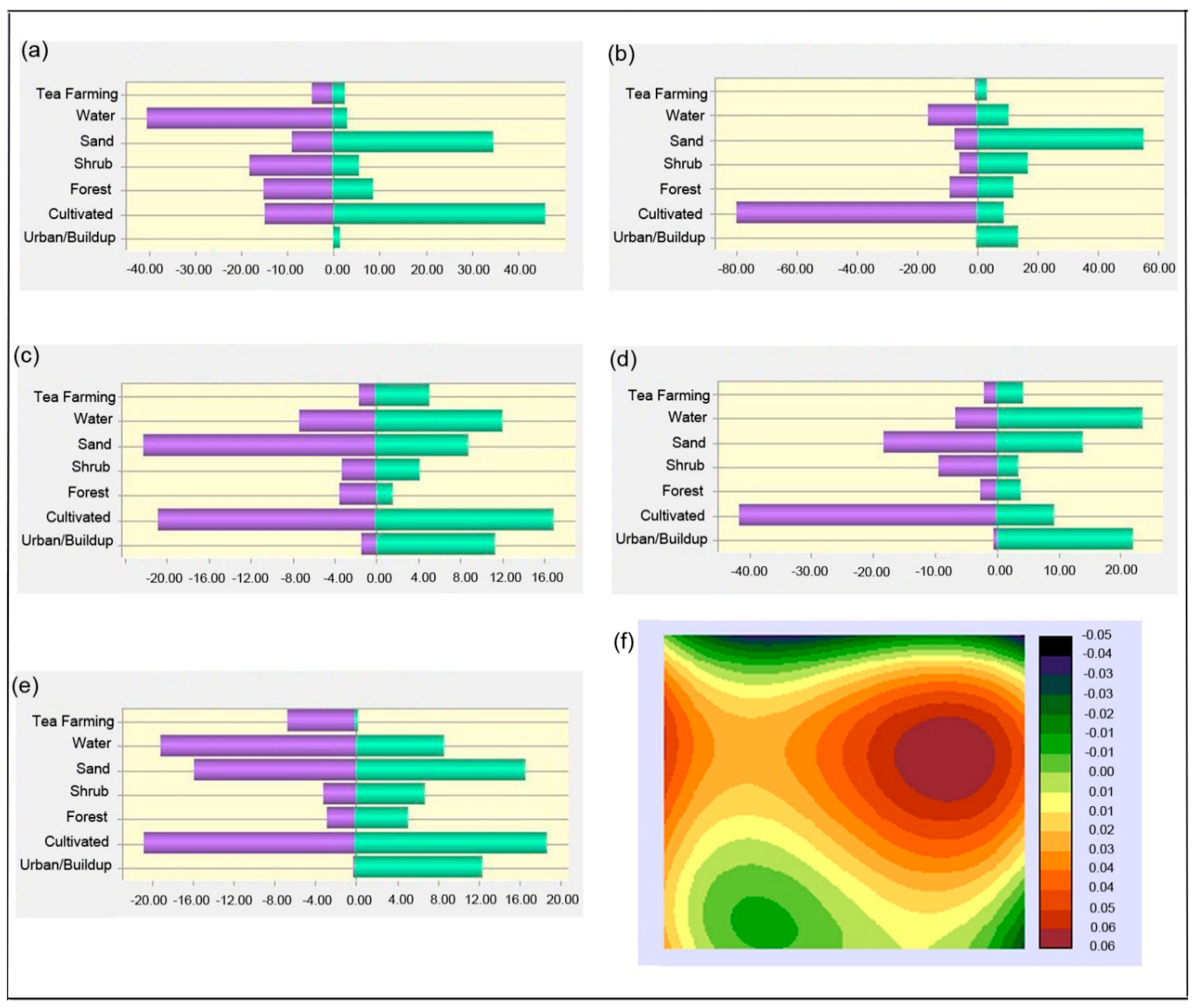
3.2. Spatial Transitions

Various natural and anthropogenic factors have resulted in LULC change and the transition ratios differ for each time period. Figure 5a–e shows the gains and losses of LULC during the period under investigation. LULC change for the district can be grouped into four stages. The first stage represents the period from 1989 to 1996 and saw a rise in cultivated area from 1259.34 to 1290.34 km2 mainly from conversion of 13.22 km2 of shrub, 12.45 km2 of forest, 9.51 km2 of water, 6.6 km2 of sand and 4.13 km2 of tea farming area. Two other major transformations were an increase in sand area from 48 to 73.76 km2 and a remarkable decline in water bodies from 71.72 to 34.40 km2 mainly due to the conversion of 29.34 km2 of water bodies to sand (Figure 5a). In the second stage from 1996 to 2001, the urban area doubled from 13.70 km2 in 1996 to 27.12 km2 in 2001 at the cost of 13.55 km2 of cultivated land. Further decreases in cultivated land to 1219.26 km2 were due to loss of forest (9.44 km2), shrubs (12.81 km2), sand (35.77 km2), water (5.34 km2) and tea (3.21 km2). Of this, 4.66 km2 of forest changed to cultivated land and 3.42 km2 to shrubs (Figure 5b).
In the third stage (2001 to 2006), 10.34 km2 of cultivated land was urbanized, 8.32 km2 of sandy area changed to cultivated land and 11.49 km2 to water, but 6.42 km2 of water changed to sand, which resulted in an overall decrease in sand from 121.26 to 107.87 km2 and increase in water from 28.61 to 33.32 km2 between 2001 and 2006 (Figure 5c). In the fourth period (from 2006 to 2011), urbanization was intense with the conversion of 20.73 km2 of cultivated land. Although the transformation of 4.48 km2 of shrubs to cultivated land occurred, the change of 6.77, 6.34 and 3.83 km2 of cultivated land to sand, water and tea, respectively, along with urban change caused an overall decrease in cultivated land. Increased population was accommodated in scattered settlements and/or the centers developed at the cost of agricultural land (Figure 5d). The final period of the study (from 2011 to 2016) was characterized by an increase in urban areas from 58.65 to 70.90 km2 with a loss of 11.45 km2 of cultivated land to urban land. The conversion of 6.26 km2 of tea farms to cultivated land demonstrated a pronounced decrease in tea farming area from 28.95 to 22.52 km2 (Figure 5e). Figure 5f shows the generalized pattern of change between 1989 and 2016 with urbanization moving outwards from the core. The darker red areas represent the more intensively changed areas which gradually decrease towards the outskirts of the city. This cubic analysis was presented using the LULC map of 1989 and 2016. The darker red areas represent the more intensively changed areas which gradually decrease towards the outskirts of the city. The eastern and western parts have more urban areas than the southern and central areas.

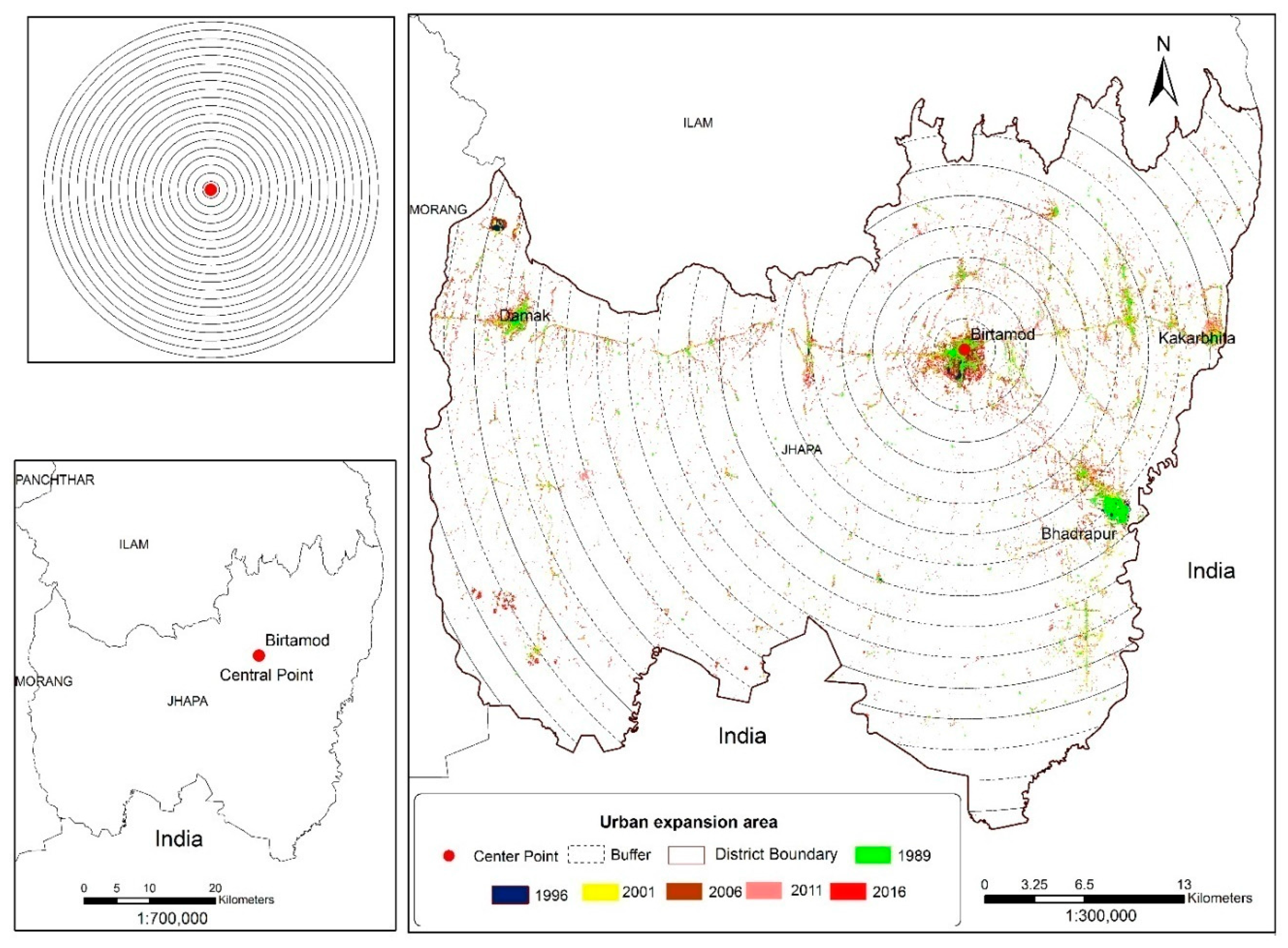
3.3. Urban Expansion

As mentioned in Section 2.4, the total extent of urban area of the region in 1989 was 12.35 km2 with an average annual growth rate of 1.56% per year in the succeeding seven years. In 1996, the urban coverage reached 13.38 km2, but sharply increased to 27.12 km2 in 2001 with the noticeable annual urban growth rate of 19.57%. It exponentially increased to 37.09 km2, but relatively decreased to 7.35% by 2006. The dramatic expansion of 58.65 km2 with an average annual growth rate of 11.63% created a historical transformation in the urban history of the district and the continuous urban expansion to 70.90 km2 with an average growth rate of 4.18% can be observed between 2011 and 2016.
Driving factors, which are defined as the underlying elements [14,35] trigger urban expansion are responsible for the urban expansion which occurs at specific temporal and spatial levels. Contextual reference is required for a better understanding of the drivers of urbanization, since distinct factors play different roles in specific time and space. Physical, socioeconomic and neighborhood factors are the main factors which directed the urbanization of Beijing; of which socioeconomic factors contributed the highest, except in the first 12 years of the study period-1972 to 2010. Also, the magnitude of physical and neighborhood factors declined as the socioeconomic factors increased [64]. Factors such as physical setting, population growth and economic development influenced urbanization in Greater Dhaka [14].
Proximate and underlying factors of public service accessibility, economic opportunity, population growth, globalization, political conditions, government plans and policies as well as social, cultural and rural urban linkages largely contributed to the migration of the population in the Nepalese context [6,65,66,67,68,69]. According to the CBS report 2014 [20], migration for agriculture (21%) was predominant over all other economic migration in rural areas, whereas service oriented migration was predominant in urban areas (17%).
The accelerated urbanization of Jhapa district is mainly driven by economic opportunity, political condition and development activities in specific periods which are further accompanied by access to public services, population growth, topography, government plans/policies and globalization factors. Such conditions are also seen in other Nepalese cities. The process of urbanization in Pokhara is mainly governed by greater economic opportunities, public service accessibility and globalization [66,68,69]. Economic opportunities in core, population growth in the fringe and political situation in the rural areas highly contributed to the urbanization process of Kathmandu valley [19]. Similarly, urban sprawl is additionally driven by physical conditions, public service accessibility and globalization as well as plans and policies [19,21,66]. The major drivers of urbanization in the rapidly urbanizing city Biratnagar are explored in Rimal, 2011 study [68] which properly reflects and represents the urbanization scenario of the Tarai region, particularly the adjoined Jhapa District.

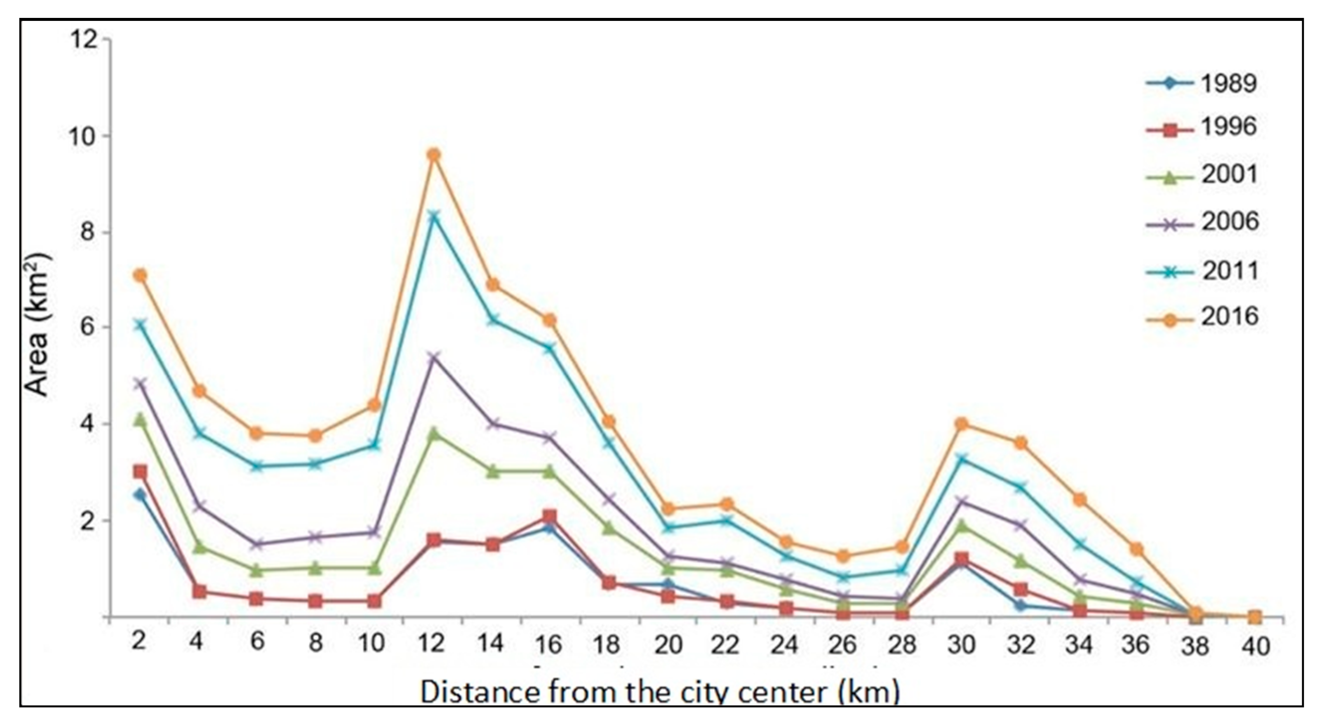
3.4. Urban Extent from City Center Outwards

In our analysis, the “center” generally refers to the urban center [52,55] and the assumed urban area gradually decreased outwards. Exploring the spatiotemporal change dynamics, orientation, cause and consequences of urban sprawl is highly essential. Nevertheless, very limited studies have outlined the contexts in terms of developing world.
The city center is usually regarded as the socioeconomic center [64]. The direction of urban expansion in the study area has been highly influenced by its socioeconomic process than its physical setting. Kakarbhitta, Birtamod, Damak and Bhadrapur are the four cities and Birtamod was assumed as the central point in our study, since it represented the largest part of urban area from the very beginning.
Ring-based analysis identified the greatest variation in the urban expansion characteristics from 1989 to 2016 (Figure 6 and Figure 7). The areas near the East-West highway and Mechi highway showed higher rates of urbanization compared to the south and south-west peripheries.
There was a gradual increase in urban area within 2–4 km of the center of Birtamod and dense settlements at Charpane and Buttabari along with the central point itself are located within these rings. The four emerging cities of Chandragadhi, Surunga, Dhulabari and Budhabare are located within ring six and Kakarbhitta in ring nine. Thus, the area from 12 to 18 km from Birtamod has experienced considerable urbanization. Consequently, the area from 28 to 32 km hold important urban coverage because the densely-settled Damak and Gauradaha are located within the specified area.

3.5. Markov Model

3.5.1. Analysis of Transition Matrix

The transition potential matrix was computed based on LULC conditions during the periods of 1996–2006, 2006–2016 and 1996–2016 to show how each land type was projected to change. Data elements lying on the diameter of the matrix indicate that a phenomenon will probably remain constant over time, while off-diagonal data indicate that various phenomena are likely to be converted to one of the other phenomena [16]. For example, the transition probability matrix shows that the probability of future loss of cultivated land to built-up area from 1996 to 2006 was 4.3%. This probability of change increased reasonably to 9% in 2016. Table 6 shows that, for both periods, cultivated land possessed the highest likelihood of transforming into built-up areas. Moreover, urban, cultivated, forest and water bodies were more likely to remain stable in the second period (2006–2016) compared to the first one (1996–2006), while other phenomena exhibited higher probabilities of changing. Tea land experienced the biggest decrease in both periods and water bodies showed the greatest increase between the first and the second projections. The likelihood of stability of land under tea cultivation decreased from 84% to 70% and the probability for most of these classes to be used for other agricultural purposes was 26% (Table 6).

3.5.2. Land-Cover Modeling and Validation

Comparison of the ground-truth map from 2016,the map simulated by the CA–Markov model using kappa variations and the Kstandard, Kno, and Klocation indicators resulted in measures of 87.5%, 90% and 94.5%, respectively. Visual comparison also shows great similarity between the two maps of 2016 (Figure 8); therefore, based on the kappa values, the CA–Markov model can be used to simulate future land-cover conditions.
The present research showed that “distance from built-up areas” played a key role in urban development. Urban development principles, access to facilities (including hospitals, schools, stores, etc.), and security priorities cause this factor to take on special importance. “Distance from main roads,” as an index of access, and “slope,” as a limiting factor, are the next effective factors in urban development, respectively (Table 2). These key drivers are usually considered by managers when solving key problems related to land-use development.

3.5.3. Analysis of Simulation Results

About 4.43% of the total land area in the region was urban in 2016 and is predicted to reach 8.11% and 10.5% by 2026 and 2036, respectively (Table 7). In contrast, cultivated land will decline from 1181.27 km2 (73.7%) to 993.61 km2 (62%), and forestland will increase from 143.01 km2 (8.9%) to 146.2 km2 (9.1%) by 2036.
Despite the urban development and population increase recorded in recent years, the expansion of agricultural lands has stopped completely in the region since about 1996 (Table 4) and expansion of urban lands has taken place instead. As shown in Figure 9, urban land will expand in the city outskirts, because agricultural land is very suitable for urban development with respect to access (proximity to built-up area) and topography [29]. Modeling further indicated an increase in natural land-cover (Natural land = Total land area − (Farmland area + Built-up area)) [70]. Natural areas are expected to cover 25.9% of the study area by 2036, which is an increase of 5.5% in comparison with the current distribution. These results are in contrast to those of Keshtkar and Voigt [60], who have shown a decrease in natural land-cover and increase in landscape fragmentation with the expansion of urban land. The increase of natural lands is mainly due to the increase of sand and shrubs. This increase is principally a result of the massive rural-urban migration and the abandonment of agricultural land. This migration can be caused by socio-economic, ecological and mismanagement drivers [71]. First, the abandoned agricultural sites converted to the bare lands and show spectral behavior like sand. Finally, the bare lands were either planted with shrubs and trees or gradually replaced by spontaneous growth of grass, shrubs, and trees via secondary succession [72,73].
The increase of natural lands confirms that management decisions were taken with the goal of protecting the natural ecosystems in the region. Although population increases and the consequent urban growth in the study region will not reduce the natural areas, they will increase landscape fragmentation. Landscape fragmentation and land holding are high in Nepal with an average of more than three parcels per holding [74]. Previous studies have shown that landscape fragmentation plays a fundamental role in reducing the connection between ecosystems [75], decreasing the possibility of migration for organisms especially for plant species [60], and increasing competition between species and their extinction [76].
Based on the authors’ local and field visit knowledge, it is explored that newer settlements have expanded onto private farmland with the direct involvement of real estate agents who purchase the land from the local owners, divide the land into smaller plots and resell them at higher rates. The rapid development of the real estate business has intensified agricultural land loss on the urban fringe because investment in the land is considered to be a secure sector. It has resulted in land fragmentation and farmland loss and fosters incompatible and disorganized land use.
The government of Nepal has introduced different land-use acts, policies, laws and regulations regarding LULC management. The National Land Use Policy of 2015 [77] emphasizes land consolidation and compact settlement to reduce land fragmentation and scattered settlements. The Settlement Development, Urban Planning and Building Construction Guidelines in 2015 provide guidance for sustainable urban planning. However, the Ministry of Urban Development (MoUD) [78] has reported that their implementation has been hindered by the lack of long-term strategies and political commitment and poor understanding of the concept of sustainability. The lack of a proper land-use plan has resulted in urban growth and loss of productive cultivable land for development [21]. Random urbanization and scattered settlements are the common features of the study area due the lack of effective urban planning.
Another harmful effect of urban development is the excessive absorption of solar radiation that worsens the urban heat island effect. Satellite studies showed that all cities in the world (especially the metropolises), are faced with this problem as a result of the materials used, especially dark-colored building materials [79]. Heat islands can directly or indirectly influence the health and social well-being of citizens. In the United States, 1000 people die annually due to heat intensity [80]. Higher temperatures, especially in summer, increase energy demand for cooling purposes, and this increase generally increases the emission of particles that pollute the air, such as greenhouse gases from power plants [81]. Moreover, population increase and urban development naturally result in an increase in the number of vehicles. The addition of each vehicle to the urban environment means that a new source of pollution has been added to the city [82]. The aforementioned problems, along with others such as global warming and scarcity of water resources, emphasize the importance of predicting the trend of urban development and the possible damage to the natural environments, so that managers can make preventive decisions if necessary.

4. Conclusions

Understanding the change in the spatial pattern of land-cover and urban growth dynamics of any area over time is important for effective land management and sustainable urban planning. Here we have described the spatiotemporal pattern of LULC and the urban expansion scenario of Jhapa district of Nepal from 1989 to 2016 with the help of multi-date images and predicted future change by 2026 and 2036 using an integrated CA–Markov model. First, the analysis explored linear urban expansion, continuous decline of cultivable land, minimum change in forest cover and shrubs, non-linear transformations of water bodies and sand and slight fluctuations in tea farming areas. Urban areas, which accounted for a total of 12.35 km2 in 1989, increased to 13.7 km2 in 1996, 27.12 km2 in 2001, 37.69 km2 in 2006, 58.65 km2 in 2011 and 70.91 km2 in 2016. This rapid urban expansion and decline of fertile agriculture land occurred mainly after 2001. Second, we explored the urban extent and orientation using ring-based analysis to show the spatiotemporal pattern of urban expansion from the urban center outwards. The rate of urban expansion has not been uniform throughout the district. Higher levels of urbanization have occurred mostly on former agricultural land near road networks and in the areas which provide quick access from the mid-hills. Urbanization was highly concentrated along the East-West and Mechi highway. Finally, using an integrated CA–Markov model, we showed that the urban area will increase to 130.12 km2 in 2026 and 167.57 km2 in 2036 while cultivated land will decline to 1085.99 and 993.61 km2 in the respective years. All other land-use classes will experience some increase.
Because massive urban expansion is ongoing at the cost of prime cultivated land and is likely to continue in future decades, food insecurity and environmental disequilibrium are probable. Developing and implementing proper urban plans for the protection of high-productive agricultural land is urgently required. Careful urban planning ensuring the preservation of cropland, green outskirts and open spaces is essential to create a resilient urban environment and sustainable development. Adopting preventive measures to dissuade high-volume immigration through various migration controls and redirection schemes should be the foremost priority of the government. The CA–Markov model is recommended as an appropriate tool for further research of the complex nature of urban and LULC. Overall, our research should serve as an important benchmark for urban planners, policy makers and other researchers.

Acknowledgments

The research was supported by the President’s International Fellowship Initiative (PIFI) of the Chinese Academy of Sciences, Grant No. 2016PE022, and the National Natural Science Foundation of China (Grant No. 41501391, 41501396). Nigel E. Stork heartily acknowledged for his support in English editing. We would like to thank Sushila Rijal for her support in developing the local level database. We would also like to thank the Editor and the anonymous reviewers for their constructive comments and suggestions.

Author Contributions

Bhagawat Rimal designed the research plan for the paper and took overall responsibility for the study, including the data collection, GIS and remote sensing analysis, preparation of figures and finalization of the manuscript. Lifu Zhang supervised the research and provided useful suggestions throughout the preparation of the manuscript. Hamidreza Keshtkar ran and analyzed the cellular automata and Markov-chain models, and edited the English language. Nan Wang and Yi Lin carried out a comprehensive revision of the article and gave useful advice. All authors revised and contributed to the final manuscript.

Conflicts of Interest

The authors declare no conflict of interest.

References

  1. Moghadam, H.S.; Helbich, M. Spatiotemporal urbanization processes in the megacity of Mumbai India: A Markov chains-cellular automata urban growth model. Appl. Geogr. 2013, 40, 140–149. [Google Scholar] [CrossRef]
  2. Ramankutty, N.; Foley, J.A. Estimating historical changes in global land cover: Croplands from 1700 to 1992. Glob. Biogeochem. Cycles 1999, 13, 997–1027. [Google Scholar] [CrossRef]
  3. Tan, M.; Li, X.; Xie, H.; Lu, C. Urban land expansion and arable land loss in China, A case study of Beijing-Tianjin-Hebei region. Land Use Policy 2005, 22, 187–196. [Google Scholar] [CrossRef]
  4. Chen, J. Rapid urbanization in China: A real challenge to soil protection and food security. Catena 2007, 69, 1–15. [Google Scholar] [CrossRef]
  5. Xu, Y.; Chan, E.H.W.; Yung, E.H.K. Overwhelming Farmland Conversion for Urban Development in Transitional China: Case Study of Shanghai. J. Urban Plan. Dev. 2014. [Google Scholar] [CrossRef]
  6. Thapa, R.B. Spatial Process of Urbanization in Kathmandu Valley, Nepal. Ph.D. Thesis, The University of Tsukuba, Tsukuba, Japan, 2009. [Google Scholar]
  7. Hyandye, C. Gis and logit regression model applications in land use/land cover change and distribution in usangu catchment. Am. J. Remote Sens. 2015, 3, 6–16. [Google Scholar] [CrossRef]
  8. UN-Habitat (United Nations Human Settlements Programme) and UN-ESCAP (United Nations Economic and Social Commission for Asia and the Pacific). The State of Asian and Pacific Cities 2015, Urban Transformations Shifting from Quantity to Quality. 2015. Available online: https://unhabitat.org/books/the-state-of-asian-and-pacific-cities-2015/ (accessed on 21 November 2016).
  9. Wu, W.J.; Zhao, S.Q.; Zhu, C.J. A comparative study of urban expansion in Beijing, Tianjin and Shijiazhuang over the past three decades. Landsc. Urban Plan. 2014, 134, 93–106. [Google Scholar] [CrossRef]
  10. Zhang, Z.; Li, N.; Wang, X.; Liu, F.; Yang, L. A Comparative Study of Urban Expansion in Beijing, Tianjin and Tangshan from the 1970s to 2013. Remote Sens. 2016, 8, 1–22. [Google Scholar] [CrossRef]
  11. Wu, J.; Jenerette, G.D.; Buyantuyev, A.; Redman, C.L. Quantifying spatiotemporal patterns of urbanization: The case of the two fastest growing metropolitan regions in the United States. J. Ecol. Complex. 2011, 8, 1–8. [Google Scholar] [CrossRef]
  12. United Nation Department of Economicand Social Affairs, P.D. World Population Prospects the 2017 Revision, Key Findings; United Nations: New York, NY, USA, 2017. [Google Scholar]
  13. United Nations Department of Economic and Social Affairs, P.D. World Urbanization Prospects the 2014 Revision, Highlights; United Nations: New York, NY, USA, 2014. [Google Scholar]
  14. Dewan, A.M.; Yamaguchi, Y. Land use and land cover change in Greater Dhaka, Bangladesh: Using remote sensing to promote sustainable urbanization. Appl. Geogr. 2009, 29, 390–401. [Google Scholar] [CrossRef]
  15. Dewan, A.M.; Yamaguchi, Y.; Rahman, M.Z. Dynamics of land use/cover changes and the analysis of landscape fragmentation in Dhaka Metropolitan, Bangladesh. GeoJournal 2012, 77, 315–330. [Google Scholar] [CrossRef]
  16. Guan, D.; Li, H.; Inohae, T.; Su, W.; Nagaie, T.; Hokao, K. Modeling urban land use change by the integration of cellular automaton and Markov model. Ecol. Model. 2011, 222, 3761–3772. [Google Scholar] [CrossRef]
  17. Su, S.; Xiao, R.; Jiang, Z.; Zhang, Y. Characterizing landscape pattern and ecosystem service value changes for urbanization impacts at an eco-regional scale. Appl. Geogr. 2012, 34, 295–305. [Google Scholar] [CrossRef]
  18. Ouyang, Z.; Fan, P.; Chen, J. Urban Built-up Areas in Transitional Economies of Southeast Asia: Spatial Extent and Dynamics. Remote Sens. 2016, 8, 1–19. [Google Scholar] [CrossRef]
  19. Thapa, R.B.; Murayama, Y. Drivers of urban growth in the Kathmandu valley, Nepal: Examining the efficacy of the analytic hierarchy process. Appl. Geogr. 2010, 30, 70–83. [Google Scholar] [CrossRef]
  20. CBS (Central Bureau of Statistics). Population Monograph of Nepal 2014. Available online: http://cbs.gov.np/population/populationmonographnepa_2014 (accessed on 29 January 2017).
  21. Rimal, B.; Zhang, L.; Fu, D.; Kunwar, R.; Zhai, Y. Monitoring urban growth and the nepal earthquake 2015 for sustainability of kathmandu valley, Nepal. Land 2017, 6, 1–23. [Google Scholar] [CrossRef]
  22. Li, X.; Yeh, A.G. Modelling sustainable urban development by the integration of constrained cellular automata and GIS. Int. J. Geogr. Inf. Sci. 2000, 14, 131–152. [Google Scholar] [CrossRef]
  23. Schneider, A. Monitoring land cover change in urban and peri-urban areas using dense time stacks of Landsat satellite data and a data mining approach. Remote Sens. Environ. 2012, 124, 689–704. [Google Scholar] [CrossRef]
  24. Jensen, J.R. Introductory Digital Processing: A Remote Sensing Perspective; Prentice-Hall: Upper Saddle River, NJ, USA, 1996. [Google Scholar]
  25. Corner, R.J.; Dewan, A.M.; Chakma, S. Monitoring and Prediction of Land-Use and Land-Cover (LULC) Change. In Dhaka Megacity, Geospatial Perspectives on Urbanization, Environment and Health; Springer Geography: Dordrecht, The Netherlands, 2013; pp. 75–97. Available online: http://www.springer.com/gp/book/9789400767348 (accessed on 17 January 2017).
  26. Hu, Z. Modeling urban growth in Atlanta using logistic regression. Comput. Environ. Urban Syst. 2007, 31, 667–688. [Google Scholar] [CrossRef]
  27. Eastman, J.R.; Solo’rzano, L.A.; Fossen, M.E.V. Transition Potential Modeling for Land Cover Change. In GIS Spatial Analysis and Modeling, 1st ed.; ESRI Press: Redlands, CA, USA, 2005; pp. 357–385. ISBN 978-1-58948-130-5. [Google Scholar]
  28. Yu, W.; Zhang, S.; Wu, C.; Liu, W.; Na, X. Analyzing and modeling land use land cover change (LUCC) in the Daqing City, China. Appl. Geogr. 2011, 31, 600–608. [Google Scholar] [CrossRef]
  29. Keshtkar, H.; Voigt, W. A spatiotemporal analysis of landscape change using integrated Markov chain cellular automata model. Model. Earth Syst. Environ. 2016, 2, 1–13. [Google Scholar] [CrossRef]
  30. Weng, Q. Land use change analysis in the Zhujiang Delta of China using satellite remote sensing, GIS and stochastic modeling. J. Environ. Manag. 2002, 64, 273–284. [Google Scholar] [CrossRef]
  31. Arsanjani, J.J.; Helbich, M.; Kainz, W.; Boloorani, A.D. Integration of logistic regression, Markov chain and cellular automata models to simulate urban expansion. Int. J. Appl. Earth Obs. Geoinf. 2013, 21, 265–275. [Google Scholar] [CrossRef]
  32. Dewan, A.M.; Islam, M.M.; Kumamoto, T.; Nishigaki, M. Evaluating Flood Hazard for Land-Use Planning in Greater Dhaka of Bangladesh Using Remote Sensing and GIS Techniques. Water Resour. Manag. 2007, 21, 1601–1612. [Google Scholar] [CrossRef]
  33. Dewan, A.M.; Kabir, M.H.; Nahar, K.; Rahman, M.Z. Urbanization and Environmental degradation in Dhaka Metropolitan Area of Bangladesh. Int. J. Environ. Sustain. Dev. 2012, 11, 118–147. [Google Scholar] [CrossRef]
  34. Byomkesh, T.; Nakagoshi, N.; Dewan, A.M. Urbanization and green space dynamics in Greater Dhaka, Bangladesh. Landsc. Ecol. Eng. 2012, 8, 45–58. [Google Scholar] [CrossRef]
  35. Rahaman, M.T. Detection of Land Use/Land Cover Changes and Urban Sprawl in Al-Khobar, Saudi Arabia: An Analysis of Multi-Temporal Remote Sensing Data. ISPRS Int. J. Geo-Inf. 2016, 5, 1–17. [Google Scholar]
  36. Cheng, J. Modelling Spatial and Temporal Urban Growth. Ph.D. Thesis, Faculty of Geo-Information Science and Earth Observation of Utrecht University, Enschede, The Netherlands, 2003, unpublished. [Google Scholar]
  37. Feng, Y.; Lu, D.; Moran, E.; Dutra, L.; Calvi, M.; de Oliveira, M. Examining spatial distribution and dynamic change of urban land covers in the brazilian amazon using multitemporal multisensor high spatial resolution satellite imagery. Remote Sens. 2017, 9, 1–20. [Google Scholar] [CrossRef]
  38. DDC (District Development Committee), Government of Nepal. District Profile; DDC: Jhapa, Nepal, 2014.
  39. USGS (United States Geological Survey) Earth Explorer, Landsat Data Archive. 2016. Available online: https://earthexplorer.usgs.gov/ (accessed on 6 September 2017).
  40. Rozenstein, O.; Qin, Z.; Derimian, Y.; Karnieli, A. Derivation of land surface temperature for Landsat-8 TIRS using a split window algorithm. Sensors 2014, 14, 5768–5780. [Google Scholar] [CrossRef] [PubMed]
  41. Zhu, Z.; Fu, Y.; Woodcock, C.E.; Olofsson, P.; Vogelmann, J.E.; Holden, C.; Wang, M.; Dai, S.; Yu, Y. Including land cover change in analysis of greenness trends using all available Landsat 5, 7, and 8 images: A case study from Guangzhou, China (2000–2014). Remote Sens Environ. 2016, 185, 243–257. [Google Scholar] [CrossRef]
  42. Google Earth Satellite Imagery of Jhapa (26°21′43′′–26°48′5′′ North to 87°38′8′′ to 88°12′00′′ East), Nepal, Images. Available online: http://earth.google.com (accessed on 8 September 2017).
  43. GoN (Government of Nepal), Ministry of Land Reform and Management: Survey Department, Topographic Survey Branch, Kathmandu. 1996. Available online: http://molrm.gov.np/ (accessed on 10 September 2017).
  44. ENVI Software, Version 4.8., ITT Visual Information Solutions, Boulder, USA. 2010. Available online: https://www.scientificcomputing.com/company-profiles/itt-visual-information-solutions (accessed on 10 September 2017).
  45. Zhou, Q.; Li, B.; Kurban, A. Trajectory analysis of land cover change in arid environment of China. Int. J. Remote Sens. 2008, 29, 1093–1107. [Google Scholar] [CrossRef]
  46. Yin, J.; Yin, Z.; Zhong, H.; Xu, S.; Hu, X.; Wang, J.; Wu, J. Monitoring urban expansion and land use/land cover changes of Shanghai metropolitan area during the transitional economy (1979–2009) in China. Environ. Monit. Assess. 2011, 177, 609–621. [Google Scholar] [CrossRef] [PubMed]
  47. Zhao, P.; Lu, D.; Wang, G.; Wu, C.; Huang, Y.; Yu, S. Examining Spectral Reflectance Saturation in Landsat Imagery and Corresponding Solutions to Improve Forest Aboveground Biomass Estimation. Remote Sens. 2016, 8, 1–26. [Google Scholar] [CrossRef]
  48. Alqurashi, A.F.; Kumar, L.; Sinha, P. Urban Land Cover Change Modelling Using Time-Series Satellite Images: A Case Study of Urban Growth in Five Cities of Saudi Arabia. Remote Sens. 2016, 8, 1–24. [Google Scholar] [CrossRef]
  49. Anderson, J.R.; Hardy, E.E.; Roach, J.T.; Witmer, R.E. A Land Use and Land Cover Classification System for Use with Remote Sensor Data; United States Government Printing Office: Washington, DC, USA, 1976.
  50. Clark Labs. TerrSet Software; Clark Labs: Worcester, MA, USA, 2016. [Google Scholar]
  51. Xiao, P.; Wang, X.; Feng, X.; Zhang, X.; Yang, Y. Detecting China’s Urban expansion over the Past Three Decades Using Nighttime Light data. IEEE Appl. Earth Obs. Remote Sens. 2014, 7, 4095–4106. [Google Scholar] [CrossRef]
  52. Wu, H.; Sun, Y.; Shi, W.; Chen, X.; Fu, D. Examining the Satellite-Detected Urban Land Use Spatial Patterns Using Multidimensional Fractal Dimension Indices. Remote Sens. 2013, 5, 51–72. [Google Scholar] [CrossRef]
  53. Jiao, L. Urban land density function: A new method to characterize urban expansion. Landsc. Urban Plan. 2015, 139, 26–39. [Google Scholar] [CrossRef]
  54. Shi, M.; Xie, Y.; Cao, Q. Spatiotemporal Change in Rural settlement land and Rural Population in Middle basin of the Heihe River China. Sustainability 2016, 8, 614. [Google Scholar] [CrossRef]
  55. Dewan, A.M.; Corner, R.J. Spatiotemporal Analysis of Urban Growth, Sprawl and Structure. In Dhaka Megacity, Geospatial Perspectives on Urbanization, Environment and Health; Springer Geography: Dordrecht, The Netherlands, 2013; pp. 99–121. Available online: http://www.springer.com/gp/book/9789400767348 (accessed on 17 January 2017).
  56. Eyoh, A.; Olayinka, D.N.; Nwilo, P.; Okwuashi, O.; Isong, M.; Udoudo, D. Modelling and Predicting Future Urban Expansion of Lagos, Nigeria from Remote Sensing Data Using Logistic Regression and GIS. Int. J. Appl. Sci. Technol. 2012, 2, 116–124. [Google Scholar]
  57. Muller, M.R.; Middleton, J. A Markov Model of land use change dynamics in the Niagara Region, Ontario, Canada. Landsc. Ecol. 1994, 9, 151–157. [Google Scholar]
  58. Sante, I.; Garcia, A.M.; Miranda, D.; Crecente, R. Cellular automata models for the simulation of real-world urban processes: A review and analysis. Landsc. Urban Plan. 2010, 96, 108–122. [Google Scholar] [CrossRef]
  59. Ward, D.P.; Murray, A.; Phinn, S.R. A stochastically constrained cellular model of urban growth. Comput. Environ. Urban Syst. 2000, 24, 539–558. [Google Scholar] [CrossRef]
  60. Keshtkar, H.; Voigt, W. Potential impacts of climate and landscape fragmentation changes on plant distributions: Coupling multi-temporal satellite imagery with GIS-based cellular automata model. Ecol. Inform. 2016, 32, 145–155. [Google Scholar] [CrossRef]
  61. Araya, Y.H.; Cabral, P. Analysis and Modeling of Urban Land Cover Change in Setúbal and Sesimbra, Portugal. Remote Sens. 2010, 2, 1549–1563. [Google Scholar] [CrossRef]
  62. Ranagalage, M.; Eastoque, R.C.; Murayama, Y. An Urban Heat Island Study of the Colombo Metropolitan Area, Sri Lanka, Based on Landsat Data (1997–2017). ISPRS Int. J. Geo-Inf. 2017, 6, 1–17. [Google Scholar] [CrossRef]
  63. Ministry of Home Affairs (MoHA). Nepal Disaster Report; Ministry of Home Affairs. Government of Nepal: Kathmandu, Nepal, 2017. Available online: http://drrportal.gov.np (accessed on 6 September 2017).
  64. Li, X.; Zhou, W.; Ouyang, Z. Forty years of urban expansion in Beijing: What is the relative importance of physical, socioeconomic, and neighborhood factors? Appl. Geogr. 2013, 38, 1–10. [Google Scholar] [CrossRef]
  65. Pradhan, P.; Perera, R. Urban growth and its impact on the livelihoods of Kathmandu valley, Nepal Urban Management Programme (UMP). Asia Occas. Pap. 2005, 63, 1–40. [Google Scholar]
  66. Rimal, B. Urban Development and Land Use Change of Main Nepalese Cities. Ph.D. Thesis, the Faculty of Earth Science and Environmental Management, University of Wroclaw, Wrocław, Poland, 2011, unpublished. [Google Scholar]
  67. Muzzini, E.; Aparicio, G. Urban Growth and Spatial Transition in Nepal, an Initial Assessment; The World Bank: Washington, DC, USA, 2013. [Google Scholar]
  68. Rimal, B. Urbanization and the decline of agricultural land in pokhara sub-metropolitan city, Nepal. J. Agric. Sci. 2012, 5, 54–56. [Google Scholar] [CrossRef]
  69. Rimal, B.; Baral, H.; Stork, N.E.; Paudyal, K.; Rijal, S. Growing City and Rapid Land Use Transition: Assessing Multiple Hazards and Risk in the Pokhara Valley Nepal. Land 2015, 4, 957–978. [Google Scholar] [CrossRef]
  70. Lambin, E.F.; Meyfroidt, P. Global land use change, economic globalization, and the looming land scarcity. Proc. Natl. Acad. Sci. USA 2011, 108, 3465–3472. [Google Scholar] [CrossRef] [PubMed]
  71. Rey Benayas, J.M.; Martins, A.; Nicolau, J.M.; Schulz, J. Abandonment of agricultural land: An overview of drivers and consequences. Perspect. Agric. Vet. Sci. Nutr. Nat. 2007, 2, 1–14. [Google Scholar] [CrossRef]
  72. Wang, C.; Gao, Q.; Wang, X.; Yu, M. Decadal Trend in Agricultural Abandonment and Woodland Expansion in an Agro-Pastoral Transition Band in Northern China. PLoS ONE 2015, 10, e0142113. [Google Scholar] [CrossRef] [PubMed]
  73. Wang, C.; Gao, Q.; Wang, X.; Yu, M. Spatially differentiated trends in urbanization, agricultural land abandonment and reclamation, and woodland recovery in northern China. Sci. Rep. 2016, 6, 37658. [Google Scholar] [CrossRef] [PubMed]
  74. Poudel, B.; Pandit, J.; Reed, B. Fragmentation and Conversion of Agriculture Land in Nepal and Land Use Policy 2012. MPRA: Munich, Germany, 2013. Available online: http://mpra.ub.uni-muenchen.de/58880/ (accessed on 6 September 2017).
  75. Meier, E.S.; Lischke, H.; Schmatz, D.R.; Zimmermann, N.E. Climate, competition and connectivity affect future migration and ranges of European trees. Glob. Ecol. Biogeogr. 2012, 21, 164–178. [Google Scholar] [CrossRef]
  76. Engler, R.; Randin, C.F.; Thuiller, W.; Dullinger, S.; Zimmermann, N.E.; Araújo, M.B.; Pearman, P.B.; Le Lay, G.; Piedallu, C.; Albert, C.H.; et al. 21st century climate change threatens mountain flora unequally across Europe. Glob. Chang. Biol. 2011, 17, 2330–2341. [Google Scholar] [CrossRef]
  77. NLUP (National Land Use Project). The National Land Use Policy; Ministry of Land Reform and Management: Kathmandu, Nepal, 2015.
  78. MoUD (Ministry of Urban Development). National Urban Development Strategy (NUDS) 2015. Available online: http://moud.gov.np/wp-content/uploads/2016/08/NUDS-2015-final-draft.pdf (accessed on 1 January 2017).
  79. Solecki, W.D.; Rosenzweig, C.; Parshall, L.; Pope, G.; Clark, M.; Cox, J.; Wiencke, M. Mitigation of the heat island effect in urban New Jersey. Glob. Environ. Chang. Part B: Environ. Hazards 2005, 6, 39–49. [Google Scholar] [CrossRef]
  80. Changnon, S.A.; Kunkel, K.E.; Reinke, B.C. Impacts and responses to the 1995 heat wave: A call to action. Bull. Am. Meteorol. Soc. 1996, 77, 1497–1506. [Google Scholar] [CrossRef]
  81. Albers, R.A.W.; Bosch, P.R.; Blocken, B.; Van Den Dobbelsteen, A.A.J.F.; Van Hove, L.W.A.; Spit, T.J.M.; Rovers, V. Overview of challenges and achievements in the Climate Adaptation of Cities and in the Climate Proof Cities program. Build. Environ. 2015, 83, 1–10. [Google Scholar] [CrossRef]
  82. California’s Advanced Clean Cars Program. Advanced Clean Cars. N.p., n.d. Web. 6 April 2014. Available online: http://www.arb.ca.gov/msprog/consumer_info/advanced_clean_cars/consumer_acc.htm (accessed on 6 September 2017).
Figure 1. Location and elevation model of study area.
Ijgi 06 00288 g001
Figure 2. Detailed framework of the study.
Ijgi 06 00288 g002
Figure 3. LULC maps of Jhapa district for 1989–2016.
Ijgi 06 00288 g003
Figure 4. Trend of LULC change in study area.
Ijgi 06 00288 g004
Figure 5. LULC transition graphs showing transition of land-cover change in km2 with losses and gains for each time period: (a) 1989 to 1996; (b) 1996 to 2001; (c) 2001 to 2006; (d) 2006 to 2011; (e) 2011 to 2016; (f) spatial trend of change (cultivated land to urban/built-up) from 1989 to 2016.
Ijgi 06 00288 g005
Figure 6. Buffer partitioning of study area.
Ijgi 06 00288 g006
Figure 7. Urban land measured from urban centers outwards.
Ijgi 06 00288 g007
Figure 8. Land-cover type in 2016: (a) actual map; (b) simulated map.
Ijgi 06 00288 g008
Figure 9. Simulated LULC maps for: (a) 2026; and (b) 2036.
Ijgi 06 00288 g009
Table 1. Land-cover classification scheme.
Land-Cover TypesDescription
Urban (Built-up)Urban and rural settlements, commercial areas, industrial areas, construction areas, traffic, airports, public service areas (e.g., school, college, hospital)
Cultivated landwet and dry crop lands, orchards
ForestEvergreen broad leaf forest, deciduous forest, scattered forest, low density sparse forest, degraded forest
ShrubMix of trees (<5 m tall) and other natural covers
SandSand area, other open field area, river bank
WaterRiver, lake/pond, canal, reservoir
TeaTea plantations
Table 2. Extracted weights based on analytic hierarchy process (AHP) and fuzzy standardization for urban areas.
FactorsFunctionsControl PointsWeights
Distance from main roadsJ-shaped0–500 m highest suitability
500–5000 m decreasing suitability
>5000 m no suitability
0.28
Distance from water bodiesLinear0–100 m no suitability
100–7500 m increasing suitability
>7500 m highest suitability
0.15
Distance from built-up areasLinear0–100 m highest suitability
100–5000 km decreasing suitability
>5000 km no suitability
0.38
SlopeSigmoid0% highest suitability
0–15% decreasing suitability
>15% no suitability
0.19
Table 3. Summary of mapping accuracy obtained by maximum likelihood classifier to the Landsat 1989, 1996, 2001, 2006, 2011 and 2016 images. OA = overall accuracy; UA = user’s accuracy; PA = producer’s accuracy.
Year198919962001200620112016
OA80.95%85.20%82.38%85.71%84.80%86.20%
PA (%)UA (%)PA (%)UA (%)PA (%)UA (%)PA (%)UA (%)PA (%)UA (%)PA (%)UA (%)
Built-up88.0085.3388.8984.0096.3189.0088.7986.6783.3381.2689.2992.53
Cultivated87.1090.0090.3293.3383.8786.6787.1090.0080.6583.3383.8786.67
Forest86.2183.3389.2983.3388.8980.0095.5983.3384.3890.0087.5093.44
Shrub77.4280.0083.3383.3380.6583.3381.2586.6780.0080.0086.2183.33
Sand81.4873.3388.8980.0076.6776.6781.8290.0083.8786.6781.8290.00
Water85.1583.3390.0091.0089.6686.6788.4676.6796.4390.0092.3180.00
Tea95.1583.3395.3086.67100.0083.3395.3086.6795.1583.3392.8686.67
Table 4. Distribution of land-use/land-cover (LULC) statistics from 1989 to 2016 (km²).
LULC198919962001200620112016
Urban12.3513.7127.1237.0958.6570.91
Cultivated1259.341290.341219.271215.431183.251181.27
Forest144.95138.57141.23139.31140.6143.01
Shrub44.8532.3142.8943.8737.9541.51
Sand48.0173.77121.26107.88103.82104.5
Water71.7234.428.6133.3350.2639.77
Tea22.2620.3823.126.5828.9622.52
Total1603.491603.491603.491603.491603.491603.49
Table 5. Magnitude of land-use/land-cover change (km²).
LULC1989–19961996–20012001–20062006–20112011–2016
Urban1.3513.429.9721.5612.26
Cultivated31−71.07−3.84−32.18−1.98
Forest−6.382.66−1.921.292.41
Shrub−12.5410.580.98−5.923.56
Sand25.7647.49−13.39−4.050.68
Water−37.32−5.794.7216.93−10.49
Tea−1.882.723.482.38−6.44
Table 6. Transition probability matrix calculated using LULC maps of 1996–2006, 2006–2016, and 1996–2016.
LULCBuilt-upCultivatedForestShrubSandWaterTea
1996–2006Built-up0.88320.11440.00000.00080.00080.00000.0008
Cultivated0.04340.84070.01590.02530.04730.01430.0130
Forest0.00520.09570.83350.05160.00930.00070.0040
Shrub0.00320.04850.09470.74050.08250.02920.0014
Sand0.00140.03250.00650.01220.80650.13550.0054
Water0.00000.01900.00000.00320.46260.51380.0013
Tea0.00470.12900.01940.00040.00300.00000.8434
2006–2016Built-up0.88640.05980.01150.01520.01960.00020.0073
Cultivated0.09010.86400.01000.01220.01320.00620.0043
Forest0.01010.03810.87900.05020.02140.00000.0011
Shrub0.02700.14400.08210.71040.02240.01370.0004
Sand0.01070.03770.00560.01180.75060.18340.0003
Water0.00140.02890.00050.00740.31430.64730.0001
Tea0.01140.26140.01420.00310.00170.00050.7077
1996–2016Built-up0.89150.10690.00000.00150.00000.00000.0000
Cultivated0.08580.81670.01700.01820.04060.01500.0067
Forest0.01420.07780.82880.06430.01410.00020.0007
Shrub0.00630.04890.14750.68340.07330.03950.0011
Sand0.00400.03290.00650.01830.76960.16570.0031
Water0.00160.01820.00190.00540.41350.55850.0009
Tea0.00970.16990.02920.00030.00030.00000.7906
Table 7. Distribution of LULC type changes for 2016–2036 (km2).
UrbanCultivatedForestShrubSandWaterTea
201670.911181.27143.0141.51104.5039.7722.52
2026130.121085.99143.4753.78112.0354.4723.63
2036167.57993.61146.2061.25150.2458.9325.70

