A Case Study of the Forced Invariance Approach for Soil Salinity Estimation in Vegetation-Covered Terrain Using Airborne Hyperspectral Imagery

Abstract

Soil spectroscopy is a promising technique for soil analysis, and has been successfully utilized in the laboratory. When it comes to space, the presence of vegetation significantly affects the performance of imaging spectroscopy or hyperspectral imaging on the retrieval of topsoil properties. The Forced Invariance Approach has been proven able to effectively suppress the vegetation contribution to the mixed image pixel. It takes advantage of scene statistics and requires no specific a priori knowledge of the referenced spectra. However, the approach is still mainly limited to lithological mapping. In this case study, the objective was to test the performance of the Forced Invariance Approach to improve the estimation accuracy of soil salinity for an agricultural area located in the semi-arid region of Northwest China using airborne hyperspectral data. The ground truth data was obtained from an eco-hydrological wireless sensing network. The relationship between Normalized Difference Vegetation Index (NDVI) and soil salinity is discussed. The results demonstrate that the Forced Invariance Approach is able to improve the retrieval accuracy of soil salinity at a depth of 10 cm, as indicated by a higher value for the coefficient of determination (R²). Consequently, the vegetation suppression method has the potential to improve quantitative estimation of soil properties with multivariate statistical methods.

1. Introduction

In arid and semi-arid areas, soil salinisation is one of the major threats to agricultural production, which could be caused by incorrect or careless irrigation [1]. The significant impacts of soil salinity on the soil-water-plant system can reduce the nutrient absorption and lead to a considerable decrease of crop productivity [2,3]. Remote sensing has been shown to be a particularly valuable tool for monitoring soil conditions frequently and spatially [4,5,6]. The presence of salts can be detected directly on bare soils with salt crust via the variation of spectral reflectance, and the spectral behaviour of salt has been studied in detail [7,8]. However, the ability to map soil salinity using the direct approach is limited, especially in agricultural areas [9,10]. The biophysical characteristics of vegetation can serve as an indirect sign of soil salinity, as plants subjected to salinity stress typically have lower photosynthetic activity, causing increased visible reflectance and reduced near-infrared reflectance from the vegetation. Therefore, various indices have been proposed for assessing and mapping soil salinity, such as the Soil Adjusted Vegetation Index (SAVI), Normalized Difference Salinity Index (NDSI) and Salinity Index (SI) [11,12,13]. Al-Khaier [14] achieved an accurate detection of soil salinity by a normalized salinity index in bare agricultural soils using ASTER bands 4 (near-infrared) and 5 (short-wave infrared). Additionally, Khan [15] successfully used NDSI with the near-infrared and red bands of the Indian Remote Sensing LISS-II sensor to map soil salinity.

Soil salinity indices usually only take advantage of a few bands, and are suitable for multispectral remote sensing images. A lot of success has been achieved in mapping severely saline areas or differentiating between saline and non-saline soils, but it is still difficult to quantitatively retrieve soil salinity [16]. Hyperspectral remote sensing or imaging spectroscopy provides high-resolution data that contains detailed spectral information of soils, and makes it possible to establish models for quantitative estimation of soil salinity. Imaging spectroscopy can not only be used for geology, water and vegetation applications, but is also a promising method for obtaining soil properties at the large scale, especially with the new hyperspectral sensors, such as EnMAP, HSUI, and HyspIRI [6,17,18,19,20].

There are many factors constraining the application of imaging spectroscopy in the field or from space, such as low signal-to-noise ratio, atmosphere attenuation, sensor resolution and Bidirectional Reflectance Distribution Functional (BRDF) effects, especially for the thin upper soil layer. Thus, optical remote sensing of soils from large distances is a significant challenge [21,22]. In the agricultural area, one of the main problems is spectral mixing. The vegetation coverage and remains might be presented in the image pixel and contribute to creating spectral confusion with soil reflectance [23,24]. Additionally, spectral absorption and reflection vary according to the type of vegetation. Therefore, removing the effects of vegetation on the soil reflectance spectra is an important research topic.

Spectral Mixture Analysis (SMA) is one of the most common techniques used to reduce the contribution of vegetation and to derive quantitative endmember abundance from hyperspectral data [25]. The HyMap hyperspectral imagery was utilised to characterise and map irrigation-induced soil salinisation, and a mixture-tuned matched filter (MTMF) approach was assessed to extract and map spectral endmembers from HyMap imagery [26]. The spectral capabilities of upcoming EnMAP were also evaluated to extract quality endmember classes that contain spectral features related to photosynthetic active vegetation (PV), non-photosynthetic active vegetation (NPV) and bare soil (BS). Estimated spectral cover can be integrated into soil erosion models using the linear unmixing method [27]. Franceschini [25] assessed pixel-fractional cover corresponding to bare soil using the linear unmixing method, and applied it to the prediction of soil properties. The model without taking into account the bare soil fractional cover showed a lower accuracy. SMA approaches often assume that endmember cover fractions contained in image pixels are linearly summed. The sub-pixel cover fraction of each land-cover endmember may be plants, bare soil or other constituents. Therefore, it is required that the observations contain enough information to solve a set of linear equations. These endmembers are usually selected either from the image data or from existing spectral libraries [28]. The problem is that referenced spectra for soils are often considered to be stable or unique, and the effects of soil properties on the spectra are not included in the models because they are unknown [29]. The Forced Invariance Approach was proposed by [30] to overcome the effects of vegetation on spectral discrimination of the underlying lithological substrate. It utilises scene statistics and requires no detailed knowledge of the reference spectra of endmembers nor any complex mixing models, and has been successfully applied in archaeology and geological mapping using multispectral and hyperspectral data [30,31,32]. However, to date, there exist few studies that have analysed whether the Forced Invariance Approach is suitable for soil spectroscopy. The accuracies of soil property estimation in the agricultural area are expected to be improved by vegetation-suppressed spectra without requiring extra field work.

The Forced Invariance Approach is focused on the production of contrast-enhanced colour composite images, which are generally used for further visual analysis and identification of lithological or urban features. Its performance on soil analysis has not been tested yet. The objective of this paper is to explore its feasibility to improve soil salinity estimation in the agricultural area. The data source was limited to airborne hyperspectral images. For the first time, the Forced Invariance Approach was adopted to improve the quantitative estimation of soil salinity at a depth of 4 cm and 10 cm by integrating eco-hydrological wireless sensor network data in an experimental agricultural area [33,34]. The possibility and the performance of vegetation suppression using the Forced Invariance Approach were discussed, and the results demonstrated that the accuracy of the determination of soil salinity at the depth of 10 cm had been improved. The vegetation suppression method is not only suitable for qualitative analysis, as used in lithological mapping, but also has the potential to improve quantitative estimation of soil properties.

2. Material and Methods

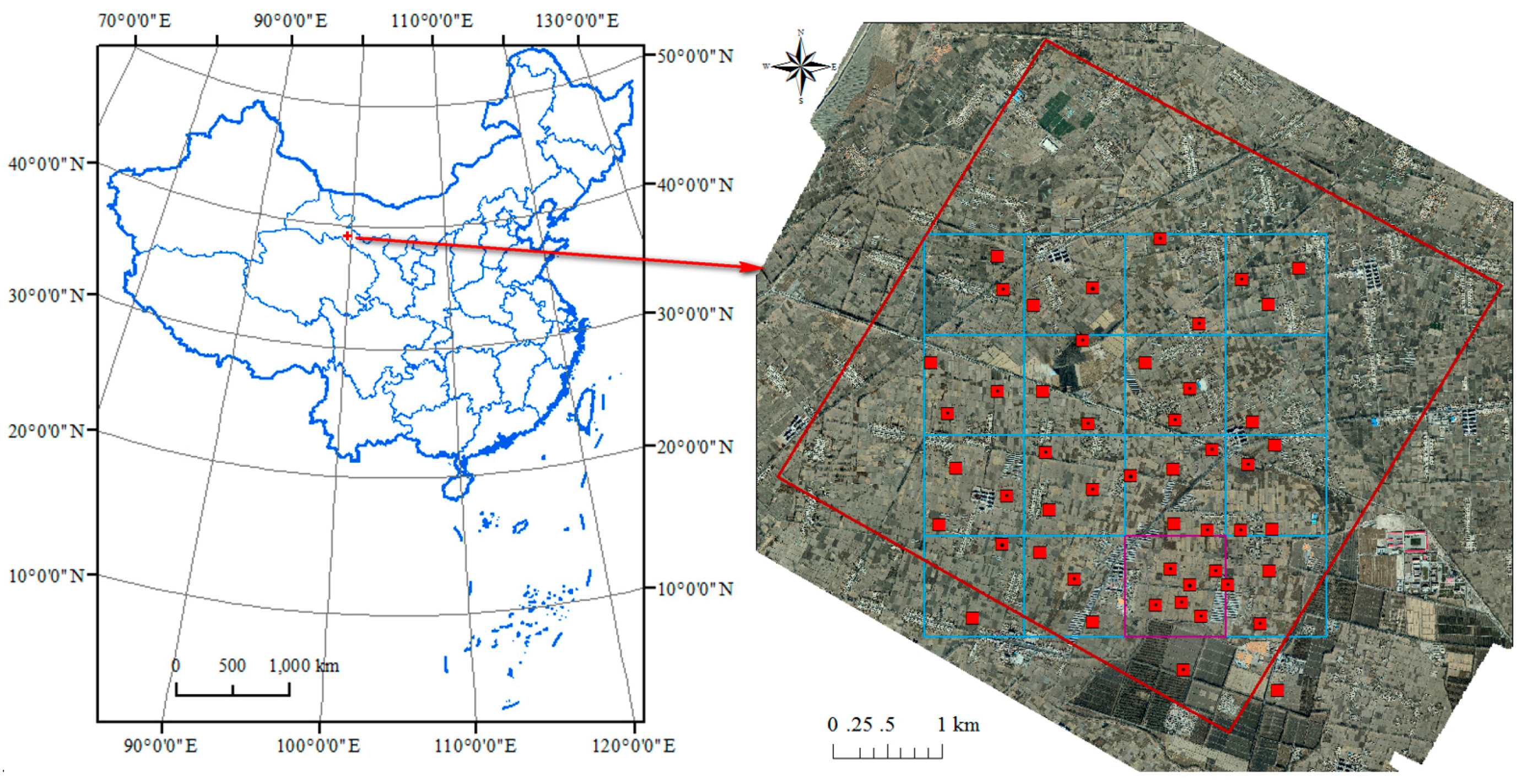
2.1. Study Area of Zhangye Oasis

The study area is located in Zhangye Oasis in the middle stream of the Chinese Heihe River Basin (100°04′ E, 39°15′ N). The oasis is located in the Gobi Desert, situated in the arid and semi-arid region of Northwest China (Figure 1) [35]. The mean annual precipitation and temperature are 121.5 mm and 6 °C, respectively. Most of the precipitation occurs between July and September. The average annual precipitation varies from 100 to 250 mm, whereas annual potential evaporation ranges from 1200 to 1800 mm, which is 10 times higher than the average annual precipitation [36]. Land cover types include wetland, grassland, and farmland. Corn is the main plant in the study area. Irrigation water in the study area is mainly supplied from the middle reaches of the Heihe River. Soil properties (bulk density, texture, and organic content) vary in the study area, and soil samples have been determined to be silt-loam with sand (9–36%), silt (56–81%), and clay (5–19%) [37].

2.2. Data Description

2.2.1. Eco-Hydrological Wireless Sensor Network Data

As part of the eco-hydrological wireless sensor network (WSN), in 2012 48 nodes were installed in the middle stream of the Heihe River Basin, covering both the Yingke and Daman irrigation districts of Zhangye Oasis (Figure 2). Data was recorded from the Hydro Probe II sensors [34] every 10 min at two different depths: 4 cm and 10 cm. Recorded information included date and time of reading, soil temperature, soil moisture, electrical conductivity (EC, soil salinity) and soil conductivity. Salinity can be viewed as the total concentration of all dissolved salts in water. Salinity can be measured by a complete chemical analysis called total dissolved solids (TDS), which is difficult and time-consuming. More often, salinity is not measured directly, but is instead derived from the conductivity measurement. There is a high correlation between electrical conductivity (EC) and total dissolved solids (TDS). In this study, we mainly use the EC values from the eco-hydrological wireless network database. The data corresponding to the date of the flight campaign were used to test the performance of the forced invariance method for the estimation of soil salinity in the agricultural area.

2.2.2. CASI Airborne Hyperspectral Data

The flight across the Heihe River Basin was conducted on 29 June 2012 at an altitude of 2000 m above, as part of the Heihe Watershed Allied Telemetry Experimental Research (HiWATER). The Compact Airborne Spectrographic Imager (CASI) 1500 developed by Itres Research Ltd. [38] was used to collect electromagnetic reflectance data. CASI 1500 is a visible and near-infrared push-broom hyperspectral sensor with 48 spectral bands covering the spectral range from 380 nm to 1050 nm. It has a field of view (FOV) of 40° with 1500 across-track imaging pixels, and the ground spatial resolution is 1.0 m. The radiometric parameter was calibrated in the calibration laboratory of the Institute of Remote Sensing and Digital Earth, Chinese Academy of Sciences, using an integrating sphere as the light source, which was developed by the Labsphere Corporation [39]. The raw data was converted from digital numbers after spectral and radiance calibration and geometrically corrected to a standard earth-centred coordinate system.

2.3. Methods

2.3.1. Vegetation Suppression Using the Forced Invariance Method

When transferring soil spectroscopy from laboratory to nature, one of the most significant issues affecting the imaging capability of spaceborne and airborne instruments is the presence of vegetation. It can obscure or even completely mask the spectral signatures of the underlying soil information. The Forced Invariance Method was originally developed by Robert Crippen and Ronald Blom (2001) [30]. It is supposed to de-correlate the vegetative component of the total signal on a pixel-by-pixel basis for each band by calculating the relationship of each input band with the vegetation index to overcome the effects of vegetation on spectral discrimination of the underlying lithological substrate. It takes advantage of information from red and near-infrared bands without requiring any specific a priori knowledge of the scene. It has been successfully used in many fields using multispectral and hyperspectral data.

In general, the idea is to fit a smooth curve to represent the relationship between the vegetation index and each band’s pixel value. By flattening these curves to a target value (such as the mean digital number value of each band), one can expect to remove the correlation with vegetation. The method can be implemented in the following sequential steps [31]: (1) dark pixel correction; (2) vegetation index calculation; (3) estimation of statistical relationship between vegetation index (VI) and digital number (DN) values for each band (Figure 3A); (4) calculation of a smooth best-fit curve for the above relationships (Figure 3B); and finally, (5) selection of a target average DN value $P_{target}$ and scaling all pixels at each vegetation index level by an amount that shifts the curve to the target DN. After curve flattening, the new value will be defined by the following equation [40]:

$$P_{new}=P_{original}\times \frac{P_{target}}{P_{NDVI}}$$

(1)

where $P_{new}$ is the vegetation-suppressed value, $P_{original}$ is the original pixel value and $P_{NDVI}$ is the NDVI corresponding value. By suppressing the vegetation component, it has the potential to reveal not only the underlying geological and archaeological features, but also soil characteristics.

The Forced Invariance Approach is based on the assumptions that (1) the distribution of vegetation across the terrain is independent of rock type, and (2) rock albedo is not substantially correlated with the vegetation amount. In our case, this means that soil properties should have no or little correlation with the vegetation index, and this is why this approach has the potential to separate the contribution of vegetation from the target pixels. NDVI was chosen as the vegetation index in the Forced Invariance Approach because it varies much more with vegetation vitality than with variations in lithological variables. Therefore, to check if the approach can be applied to soil analysis, the correlation between NDVI and soil salinity should be examined. Soil moisture is also a major concern for agriculture. Engstrom (2008) [41] already pointed out that the correlation between soil moisture and NDVI was not significant in areas with little to no relief.

2.3.2. Spectral Modelling of Soil Properties

The relationship between spectra extracted from the hyperspectral image and soil properties was analysed using the Generalized Linear Model (GLM). The GLM is a flexible generalisation of ordinary linear regression that allows for response variables that have error distribution models other than a normal distribution. The study results from Yuan Huang [42] show that soil moisture, EC and clay content were log-normally distributed, while organic carbon, sand and silt content were normally distributed. Therefore, the Logit Link Function was chosen to model the correlation between spectral data and soil salinity in this study.

Each pixel spectrum of the hyperspectral image comprehends a total of 48 bands, which would cause redundancy of information. Minimum Noise Fraction (MNF) is one of the most common methods to extract features from hyperspectral data, and can effectively reduce a large dataset into a smaller number of components that contain the majority of information. Therefore, MNF transform was performed on the mosaicked and subtracted airborne hyperspectral data using the ENvironment for Visualizing Images (ENVI) software. The data acquired by the vegetation suppression method was also transformed by MNF. The first 14 MNF components were retained as the input variables.

2.4. Model Performance Assessment

For each soil property, the soil spectral quantitative model was developed on a random sample of two-thirds of the data using the GLM. The calibrations were tested by predicting the soil salinity (EC) on validation data sets composed of the remaining one third of samples. The model accuracies were evaluated on estimated and measured soil salinity using RMSE and R².

$$R^2=\frac{{\sum }_{i=1}^n{\left({\widehat{y}}_i-\overline{y}\right)}^2}{{\sum }_{i=1}^n{\left(Y_i-\overline{Y}\right)}^2}$$

(2)

$$\mathrm{RMSE}=\sqrt{\frac{1}{n}{\sum }_{i=1}^n{\left({\widehat{y}}_i-y_i\right)}^2}$$

(3)

where n is the number of validation samples, y represents the measured values, $\overline{y}$ is the mean of the measured values, and $\widehat{y}$ is the estimated values.

3. Results and Discussion

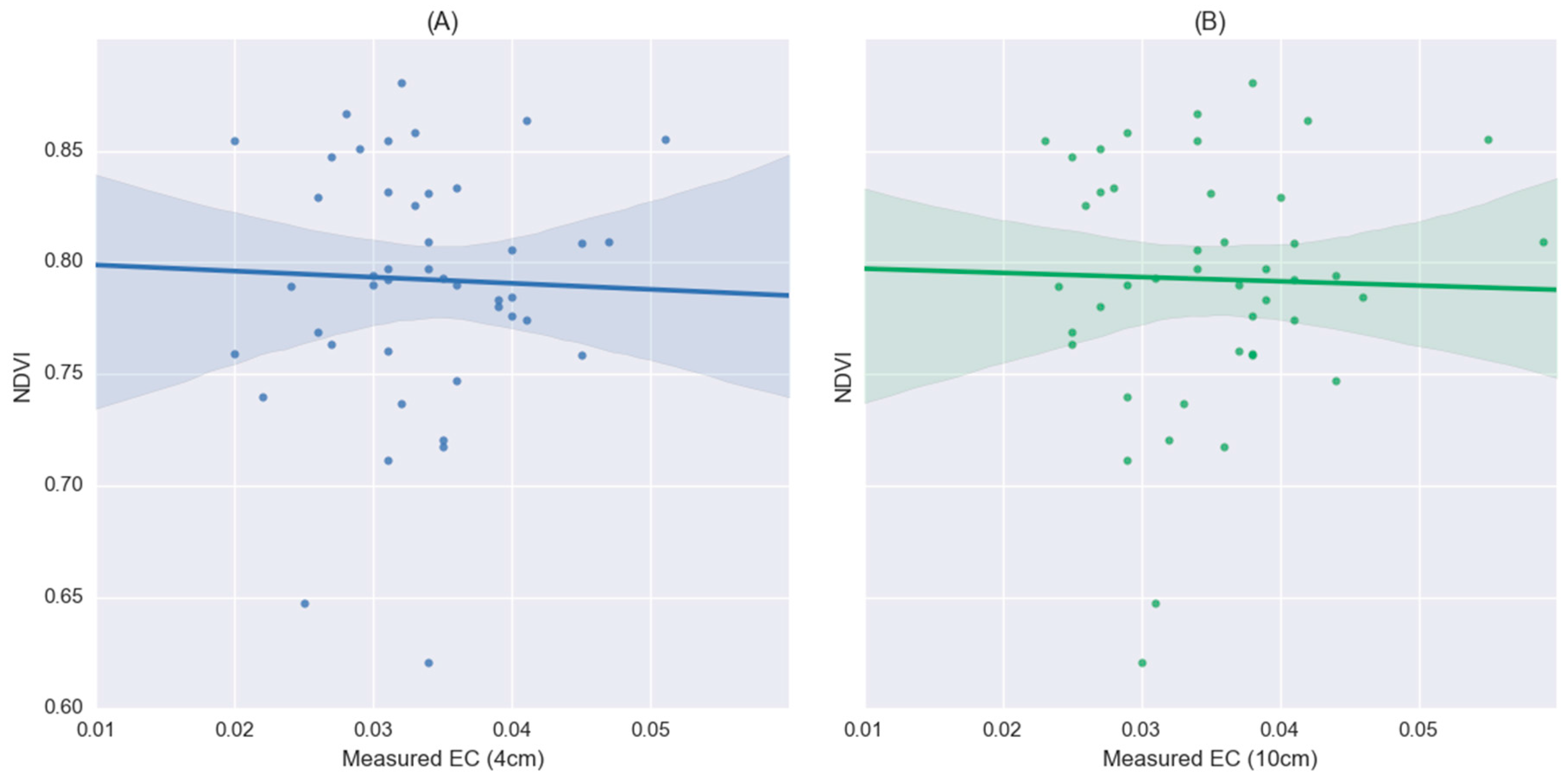
3.1. Correlation between NDVI and Soil Salinity

The terrain in Zhangye Oasis is relatively flat. The correlation between NDVI and soil salinity at the depths of 4 cm and 10 cm are shown in Figure 4. The deviation from the fitted line demonstrated that NDVI basically has little correlation with soil salinity either at the depth of 10 cm or 4 cm. The Pearson values between NDVI and soil salinity were also calculated. The correlation at the depth of 4 cm has a slightly higher value (r = 0.042) than at the depth of 10 cm (r = 0.032).

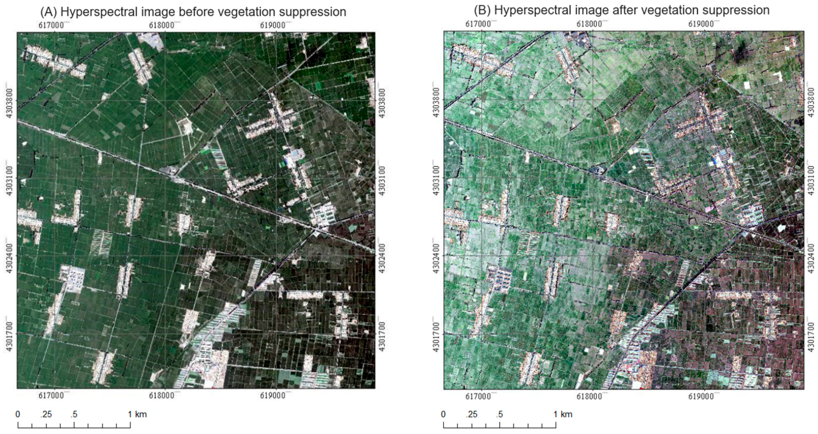
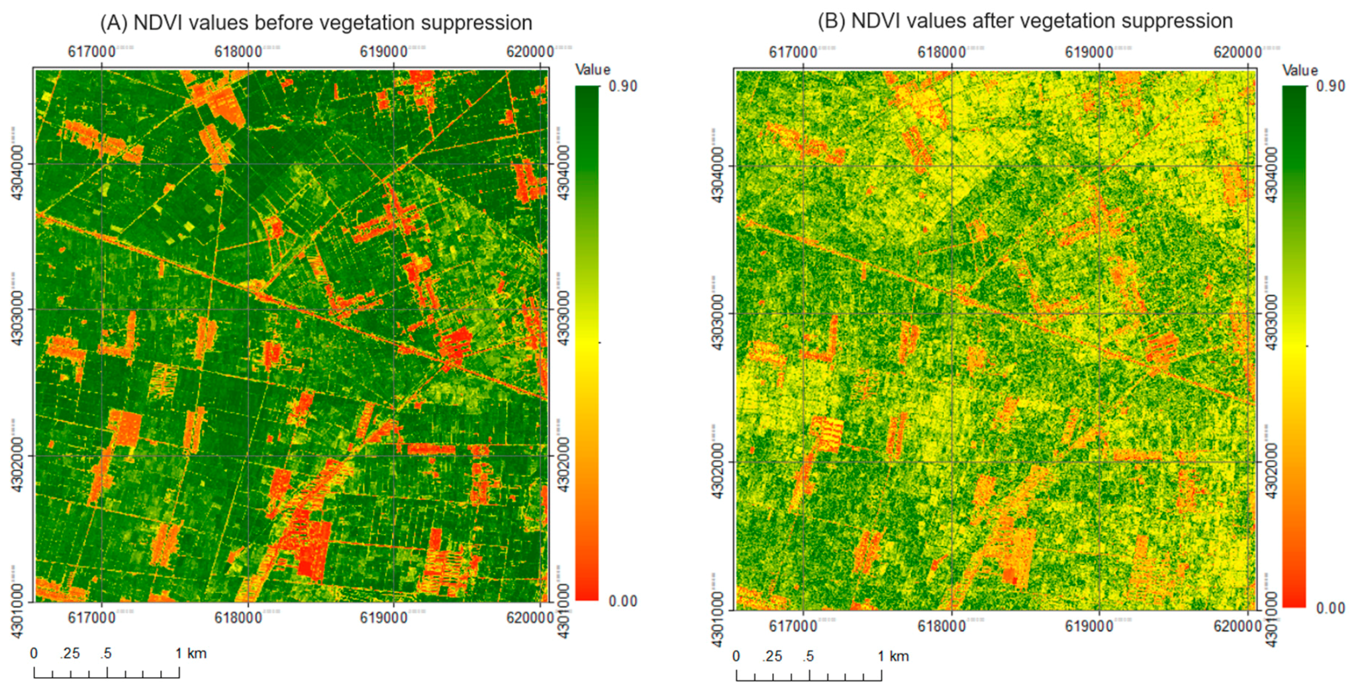
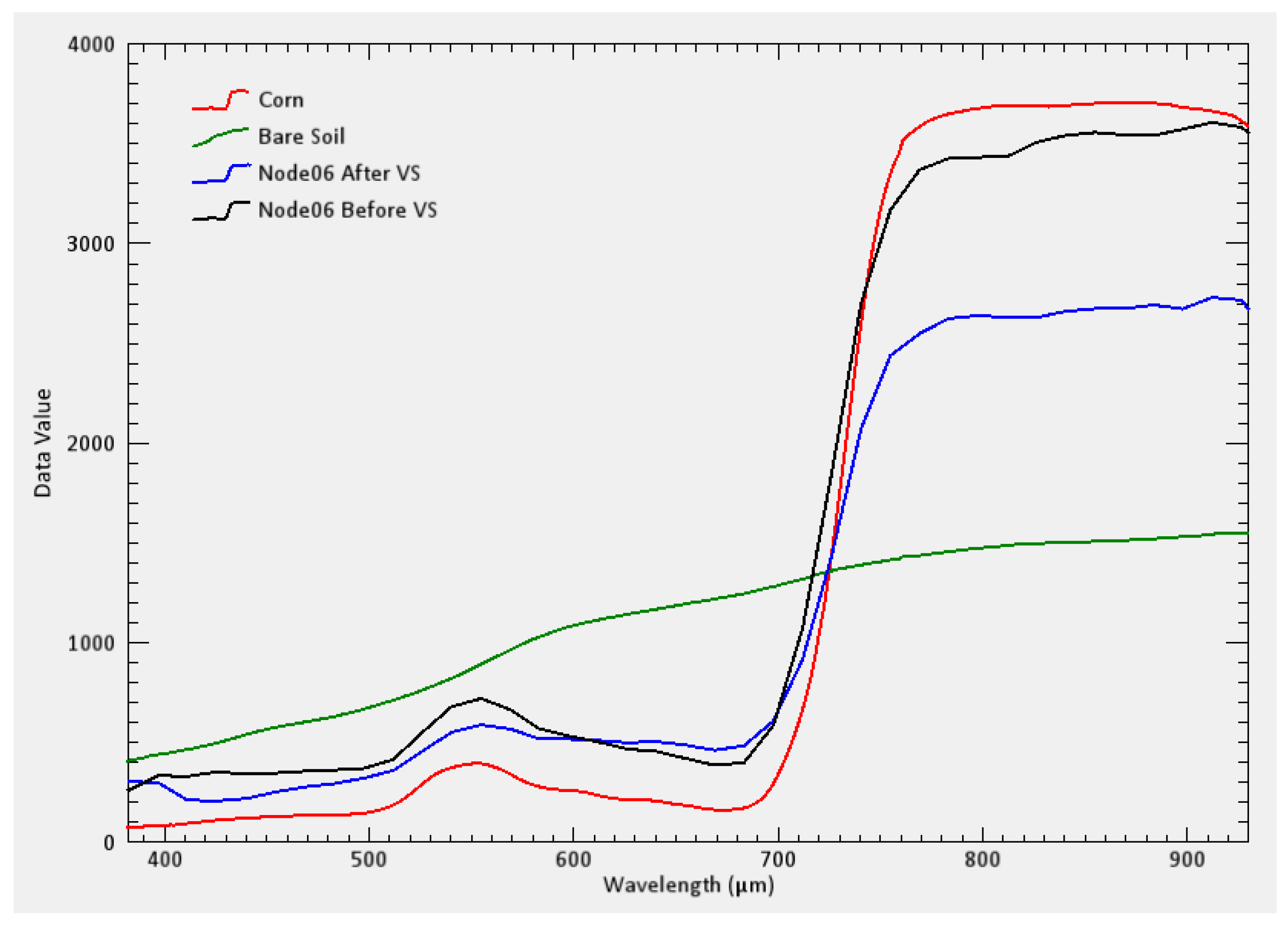
3.2. Vegetation Suppression Performance Using the Forced Invariance Approach

The vegetation cover, which is mainly corn in the study area, could hinder the acquisition of spectral signatures of the underlying soil information. The Forced Invariance Method is assumed to be applicable to the suppression of vegetation. From Section 3.1, we know that it is possible to take advantage of this method to enhance the soil information from the mixed spectra. To check the performance of the vegetation suppression method, the easiest way is to check the true colour image (false colour image is an alternative way) with the naked eye. It can be seen that, while the original image (Figure 5A) is dominated by vegetation, the green hue is not so obvious in the processed image (Figure 5B), and the latter one also shows some bare soil spots. Another approach is to take advantage of the NDVI, which is one of the most useful vegetation indices. By comparing Figure 6A,B it can be seen that the NDVI values are also significantly reduced.

As the dataset used in this study represents airborne hyperspectral imagery, we can further examine the effect of the Forced Invariance Approach using spectral lines. The corn and bare soil spectra measured by ASD Field Spec3 (obtained from the Heihe Plan Science Data Centre) were taken as pure endmembers. The acquired spectra were compared to the spectra extracted from hyperspectral images at the pixel corresponding to sensor node 06 before and after vegetation suppression. A comparison of the spectra is shown in Figure 7. The soil spectrum has no obvious absorption features. Although the spectrum from hyperspectral imagery at the specified pixel after vegetation suppression still has a similar shape with corn spectrum, the slop of “red edge” was reduced in height.

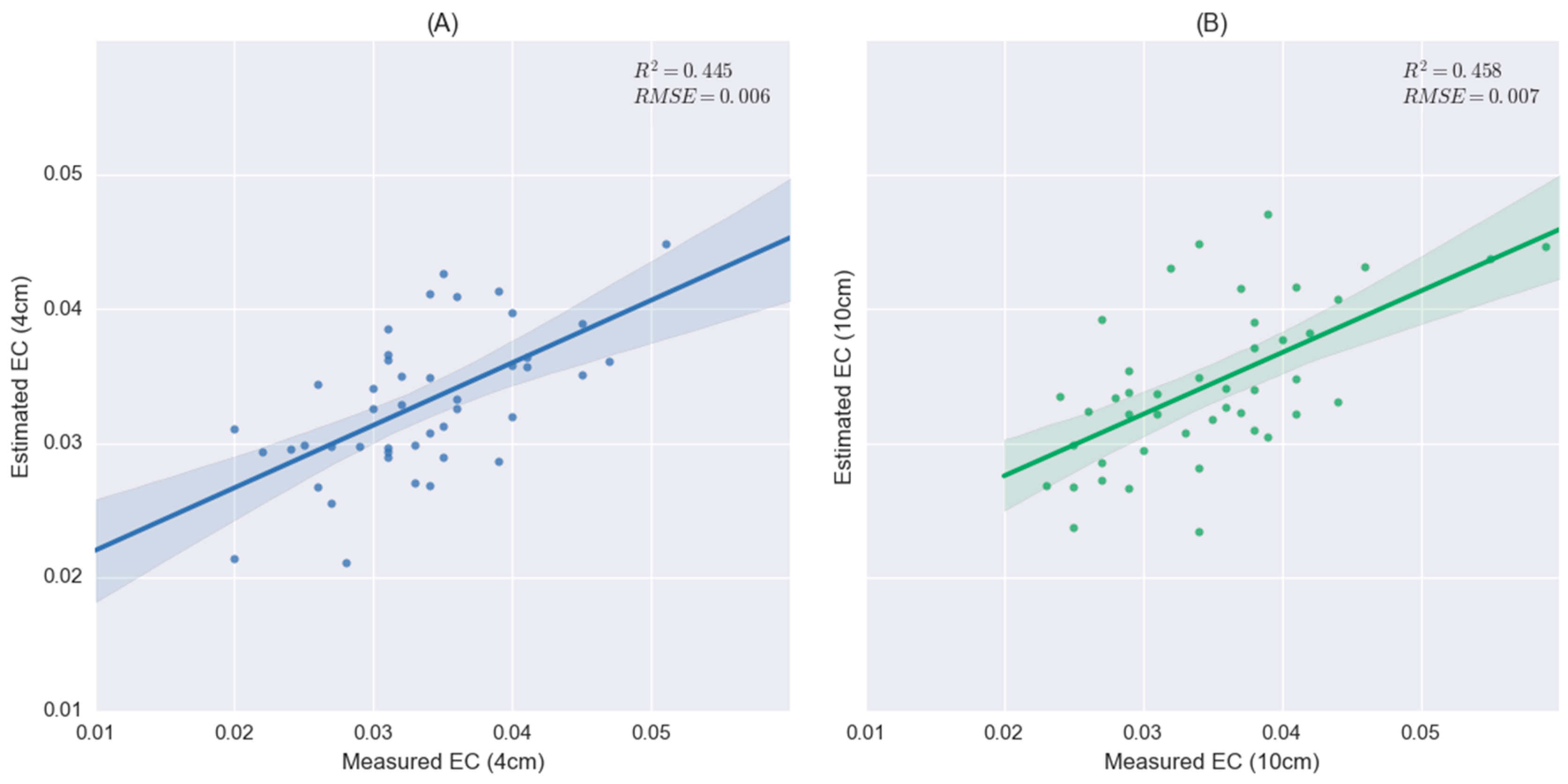
3.3. Estimation of Soil Properties Using Airborne Hyperspectral Data

To quantitatively evaluate the performance of the Forced Invariance Approach using airborne hyperspectral data for agriculture, the relationship between soil spectra and soil salinity were modelled using the GLM. The accuracy of soil salinity at a depth of 10 cm (R² = 0.458) is slightly higher than at a depth of 4 cm (R² = 0.445) using hyperspectral data without vegetation suppression (Figure 8), which is more obvious for results obtained from data with vegetation suppression (Figure 9). The reason for this is that surface soil is significantly influenced by exterior factors like irrigation and wind, and landscape fragmentation and complicated cultivation structures also contribute to the high spatial heterogeneity of the soil properties. Therefore, it is less stable and more heterogeneous at a depth of 4 cm than soil at 10 cm.

By comparing Figure 8 and Figure 9, it can be seen that the accuracies for the estimation of soil salinity at the depth of 10 cm (R² = 0.538) improved significantly after applying the Forced Invariance Approach, but not like at a depth of 4 cm (R² = 0.43). Apart from the high spatial heterogeneity for surface soil properties, this might also be caused by the correlation to the NDVI. Although the correlation of soil salinity to NDVI was not significant, as revealed by Figure 4, soil properties at a depth of 4 cm still showed a higher correlation value than at a depth of 10 cm. The modelling results showed that this approach performed better for soil salinity at a depth of 10 cm, which is in agreement with the assumption that the target property should have no or little correlation with the vegetation index. However, it does not guarantee that the model’s accuracy will be improved with the increase of soil depth due to limited effective penetration depth of optical sensors.

4. Conclusions

The spatial distribution of soil salinity has important implications for soil and water resource management in arid and semi-arid agricultural regions. The present study examines the possibility of improving the estimation accuracy of soil salinity at different soil depths using imaging spectroscopy and vegetation suppression based on the Forced Invariance Approach, which calculates images that are invariant relative to a specific spectral index, and where features represented by that spectral index will not appear in the resulting images because those features will not contribute to the variance.

The relationship between NDVI and soil salinity in the study area indicates that there exists no significant correlation. The GLM developed using wireless network data and airborne hyperspectral data shows a better performance for soil salinity estimation at the depth of 10 cm than at 4 cm, and to the estimation accuracy (R² = 0.538) for soils at a depth of 10 cm after vegetation suppression improved when compared to the result (R² = 0.458) obtained from the model built using hyperspectral data without vegetation suppression. However, the approach failed for soils at a depth of 4 cm. Hence, one should check carefully before applying the Forced Invariance Approach to improve quantitative soil analysis. In addition, the main drawback of the vegetation suppression algorithm is a severe distortion of the spectral values in non-vegetated areas. The masking technique should be considered in the mapping procedure to keep pixel values from bare soil or sparse vegetation unchanged. The presence of vegetation restrains the application of hyperspectral imagery in retrieving underlying soil properties. The Forced Invariance Approach can not only produce contrast-enhanced colour composite images for lithological mapping but also has the potential to contribute to the retrieval of soil properties with multivariate statistical methods.

References

1. Douaoui, A.E.K.; Nicolas, H.; Walter, C. Detecting salinity hazards within a semiarid context by means of combining soil and remote-sensing data. Geoderma 2006, 134, 217–230. [Google Scholar] [CrossRef]
2. Alexakis, D.; Gotsis, D.; Giakoumakis, S. Evaluation of soil salinization in a Mediterranean site (Agoulinitsa district-West Greece). Arabian J. Geosci. 2014, 8, 1373–1383. [Google Scholar] [CrossRef]
3. Fourati, H.T.; Bouaziz, M.; Benzina, M.; Bouaziz, S. Modeling of soil salinity within a semi-arid region using spectral analysis. Arabian J. Geosci. 2015, 8, 11175–11182. [Google Scholar] [CrossRef]
4. Biro, K.; Pradhan, B.; Buchroithner, M.; Makeschin, F. Land use/land cover change analysis and its impact on soil properties in the northern part of Gadarif region, Sudan. Land Degrad. Dev. 2013, 24, 90–102. [Google Scholar] [CrossRef]
5. Biro, K.; Pradhan, B.; Sulieman, H.; Buchroithner, M. Exploitation of TerraSAR-X data for land use/land cover analysis using object-oriented classification approach in the African Sahel Area, Sudan. J. Indian Soc. Remote Sens. 2013, 41, 539–553. [Google Scholar] [CrossRef] [Green Version]
6. Nocita, M.; Stevens, A.; van Wesemael, B.; Aitkenhead, M.; Bachmann, M.; Barthès, B.; Ben-Dor, E.; Brown, D.J.; Clairotte, M.; Csorba, A.; et al. Soil spectroscopy: An alternative to wet chemistry for soil monitoring. Adv. Agron. 2015, 132, 139–159. [Google Scholar]
7. Asfaw, E.; Suryabhagavan, K.V.; Argaw, M. Soil salinity modeling and mapping using remote sensing and GIS: The case of Wonji sugar cane irrigation farm, Ethiopia. J. Saudi Soc. Agric. Sci. 2016. [Google Scholar] [CrossRef]
8. Metternicht, G.I.; Zinck, J.A. Remote sensing of soil salinity: Potentials and constraints. Remote Sens. Environ. 2003, 85, 1–20. [Google Scholar] [CrossRef]
9. Allbed, A.; Kumar, L. Soil salinity mapping and monitoring in arid and Semi-arid regions using remote sensing technology: A review. Adv. Remote Sens. 2013, 2, 373–385. [Google Scholar] [CrossRef]
10. Zhang, T.; Qi, J.; Gao, Y.; Ouyang, Z.; Zeng, S.; Zhao, B. Detecting soil salinity with MODIS time series VI data. Ecol. Indic. 2015, 52, 480–489. [Google Scholar] [CrossRef]
11. Tilley, D.R.; Ahmed, M.; Son, J.H.; Badrinarayanan, H. Hyperspectral reflectance response of freshwater macrophytes to salinity in a brackish subtropical marsh. J. Environ. Qual. 2007, 36, 780. [Google Scholar] [CrossRef] [PubMed]
12. Huete, A. A soil-adjusted vegetation index (SAVI). Remote Sens. Environ. 1988, 25, 295–309. [Google Scholar] [CrossRef]
13. Bannari, A.; Guedon, A.M.; El-Harti, A.; Cherkaoui, F.Z.; El-Ghmari, A. Characterization of slightly and moderately saline and sodic soils in irrigated agricultural land using simulated data of advanced land imaging (EO-1) sensor. Commun. Soil Sci. Plant Anal. 2008, 39, 2795–2811. [Google Scholar] [CrossRef]
14. Al-Khaier, F. Soil Salinity Detection Using Satellite Remote Sensing. Master’s Thesis, International Institute for Geo-Information Science and Earth Observation, Enschede, The Netherlands, 2003. [Google Scholar]
15. Khan, N.M.; Rastoskuev, V.V.; Sato, Y.; Shiozawa, S. Assessment of hydrosaline land degradation by using a simple approach of remote sensing indicators. Agric. Water Manag. 2005, 77, 96–109. [Google Scholar] [CrossRef]
16. Weng, Y.-L.; Gong, P.; Zhu, Z.-L. A spectral index for estimating soil salinity in the Yellow River Delta region of China using EO-1 Hyperion data. Pedosphere 2010, 20, 378–388. [Google Scholar] [CrossRef]
17. Guanter, L.; Kaufmann, H.; Segl, K.; Foerster, S.; Rogass, C.; Chabrillat, S.; Kuester, T.; Hollstein, A.; Rossner, G.; Chlebek, C.; et al. The EnMAP spaceborne imaging spectroscopy mission for earth observation. Remote Sens. 2015, 7, 8830–8857. [Google Scholar] [CrossRef] [Green Version]
18. Hochberg, E.J.; Roberts, D.A.; Dennison, P.E.; Hulley, G.C. Special issue on the Hyperspectral Infrared Imager (HyspIRI): Emerging science in terrestrial and aquatic ecology, radiation balance and hazards. Remote Sens. Environ. 2015, 167, 1–5. [Google Scholar] [CrossRef]
19. Liu, L.; Ji, M.; Buchroithner, M. Combining partial least squares and the gradient-boosting method for soil property retrieval using visible near-infrared shortwave infrared spectra. Remote Sens. 2017, 9, 1299. [Google Scholar] [CrossRef]
20. Liu, L.; Ji, M.; Dong, Y.; Zhang, R.; Buchroithner, M. Quantitative retrieval of organic soil properties from visible near-infrared Shortwave infrared (Vis-NIR-SWIR) spectroscopy feature extraction. Remote Sens. 2016, 8, 1035. [Google Scholar] [CrossRef]
21. Ben-Dor, E.; Taylor, R.G.; Hill, J.; Demattê, J.A.M.; Whiting, M.L.; Chabrillat, S.; Sommer, S. Imaging spectrometry for soil applications. Adv. Agron. 2008, 97, 321–392. [Google Scholar]
22. Ben-Dor, E.; Chabrillat, S.; Demattê, J.A.M.; Taylor, G.R.; Hill, J.; Whiting, M.L.; Sommer, S. Using imaging spectroscopy to study soil properties. Remote Sens. Environ. 2009, 113, S38–S55. [Google Scholar] [CrossRef]
23. Palacios-Orueta, A.; Pinzon, J.E.; Ustin, S.L.; Roberts, D.A. Remote sensing of soils in the Santa Monica Mountains: II. Hierarchical foreground and background analysis. Remote Sens. Environ. 1999, 68, 138–151. [Google Scholar] [CrossRef]
24. Mashimbye, Z.E.; Cho, M.A.; Nell, J.P.; De Clercq, W.P.; Van Niekerk, A.; Turner, D.P. Model-Based integrated methods for quantitative estimation of soil salinity from hyperspectral remote sensing data: A case study of selected south African soils. Pedosphere 2012, 22, 640–649. [Google Scholar] [CrossRef]
25. Franceschini, M.H.D.; Demattê, J.A.M.; da Silva Terra, F.; Vicente, L.E.; Bartholomeus, H.; de Souza Filho, C.R. Prediction of soil properties using imaging spectroscopy: Considering fractional vegetation cover to improve accuracy. Int. J. Appl. Earth Obs. Geoinf. 2015, 38, 358–370. [Google Scholar] [CrossRef]
26. Dehaan, R.; Taylor, G.R. Image-derived spectral endmembers as indicators of salinisation. Int. J. Remote Sens. 2003, 24, 775–794. [Google Scholar] [CrossRef]
27. Malec, S.; Rogge, D.; Heiden, U.; Sanchez-Azofeifa, A.; Bachmann, M.; Wegmann, M. Capability of spaceborne hyperspectral EnMAP mission for mapping fractional cover for soil erosion modeling. Remote Sens. 2015, 7, 11776–11800. [Google Scholar] [CrossRef] [Green Version]
28. Asner, G.P.; Heidebrecht, K.B. Spectral unmixing of vegetation, soil and dry carbon in arid regions: Comparing multispectral and hyperspectral observations. Int. J. Remote Sens. 2001, 23, 3939–3958. [Google Scholar] [CrossRef]
29. Muller, E.; Décamps, H. Modeling soil moisture–reflectance. Remote Sens. Environ. 2000, 76, 173–180. [Google Scholar] [CrossRef]
30. Crippen, R.E.; Blom, R.G. Unveiling the lithology of vegetated terrains in remotely sensed imagery. Photogramm. Eng. Remote Sens. 2001, 91109, 935–943. [Google Scholar]
31. Yu, L.; Porwal, A.; Holden, E.-J.; Dentith, M.C. Suppression of vegetation in multispectral remote sensing images. Int. J. Remote Sens. 2011, 32, 7343–7357. [Google Scholar] [CrossRef]
32. Evans, D.; Traviglia, A. Uncovering Angkor: Integrated remote sensing applications in the archaeology of early Cambodia. In Satellite Remote Sensing: A New Tool for Archaeology; Lasaponara, R., Masini, N., Eds.; Springer: Berlin/Heidelberg, Germany, 2003; pp. 197–230. [Google Scholar]
33. Kang, J.; Li, X.; Jin, R.; Ge, Y.; Wang, J.; Wang, J. Hybrid optimal design of the eco-hydrological wireless sensor network in the middle reach of the Heihe River Basin, China. Sensors 2014, 14, 19095–19114. [Google Scholar] [CrossRef] [PubMed]
34. Jin, R.; Li, X.; Yan, B.; Li, X. A nested ecohydrological wireless sensor network for capturing the surface heterogeneity in the midstream areas of the Heihe River Basin, China. IEEE Geosci. Remote Sens. Lett. 2015, 11, 2015–2019. [Google Scholar] [CrossRef]
35. Meng, J.; Long, H. Water resources in oasis ecological balance: The case of Zhangye Oasis. Chin. J. Arid Land Res. 1998, 11, 255–262. [Google Scholar]
36. Li, X.; Cheng, G.; Liu, S.; Xiao, Q.; Ma, M.; Jin, R.; Che, T.; Liu, Q.; Wang, W.; Qi, Y.; et al. Heihe watershed allied telemetry experimental research (HiWater) scientific objectives and experimental design. Bull. Am. Meteorol. Soc. 2013, 94, 1145–1160. [Google Scholar] [CrossRef]
37. Xiaodong, S.; Ganlin, Z.; Feng, L.I.U.; Decheng, L.I.; Yuguo, Z.; Jinling, Y. Modeling spatio-temporal distribution of soil moisture by deep learning-based cellular automata model. J. Arid Land 2016, 8, 734–748. [Google Scholar]
38. Guanter, L.; Estellés, V.; Moreno, J. Spectral calibration and atmospheric correction of ultra-fine spectral and spatial resolution remote sensing data. Application to CASI-1500 data. Remote Sens. Environ. 2007, 109, 54–65. [Google Scholar] [CrossRef]
39. Li, X.; Liu, S.; Xiao, Q.; Ma, M.; Jin, R.; Che, T.; Wang, W. A multiscale dataset for understanding complex eco-hydrological processes in a heterogeneous oasis system. Sci. Data 2017, 4, 1–11. [Google Scholar] [CrossRef] [PubMed]
40. Hede, A.N.H.; Koike, K.; Kashiwaya, K.; Sakurai, S.; Yamada, R.; Singer, D.A. How can satellite imagery be used for mineral exploration in thick vegetation areas? Geochem. Geophys. Geosyst. 2017, 18, 584–596. [Google Scholar] [CrossRef]
41. Engstrom, R.; Hope, A.; Kwon, H.; Stow, D. The relationship between soil moisture and NDVI near Barrow, Alaska. Phys. Geogr. 2008, 29, 38–53. [Google Scholar] [CrossRef]
42. Huang, Y.; Wang, Y.; Zhao, Y.; Xu, X.; Zhang, J.; Li, C. Spatiotemporal distribution of soil moisture and salinity in the Taklimakan Desert highway shelterbelt. Water 2015, 7, 4343–4361. [Google Scholar] [CrossRef]
Figure 1. Location of study area and the distribution of wireless sensor network nodes.
Ijgi 07 00048 g001
Figure 2. Sensor node and router of the wireless sensor network.
Ijgi 07 00048 g002
Figure 3. Scatter plot (A) and best-fit curve (B) of Normalized Difference Vegetation Index (NDVI) and digital number (DN) values.
Ijgi 07 00048 g003
Figure 4. Correlation between NDVI soil salinity (EC) at the depths of 4 cm (A) and 10 cm (B).
Ijgi 07 00048 g004
Figure 5. Comparison of airborne hyperspectral true colour images (R: 640.5 nm, G: 554.7 nm B: 468.7 nm) before (A) and after vegetation suppression (B).
Ijgi 07 00048 g005
Figure 6. Comparison of NDVI values of airborne hyperspectral images before (A) and after vegetation suppression (B).
Ijgi 07 00048 g006
Figure 7. Comparison between measured corn and bare soil spectra and the spectra at the location of the specified sensor node from hyperspectral images before and after vegetation suppression.
Ijgi 07 00048 g007
Figure 8. Regression plots between measured target values and estimated values before vegetation suppression for soil salinity at the depth of 4 cm (A) and 10 cm (B).
Ijgi 07 00048 g008
Figure 9. Regression plots between measured target values and estimated values after vegetation suppression for soil salinity at the depth of 4 cm (A) and 10 cm (B).
Ijgi 07 00048 g009