A Regional Mapping Method for Oilseed Rape Based on HSV Transformation and Spectral Features

Abstract

This study proposed a colorimetric transformation and spectral features-based oilseed rape extraction algorithm (CSRA) to map oilseed rape at the provincial scale as a first step towards country-scale coverage. Using a stepwise analysis strategy, our method gradually separates vegetation from non-vegetation, crop from non-crop, and oilseed rape from winter wheat. The wide-field view (WFV) images from Chinese Gaofen satellite no. 1 (GF-1) at six continuous flowering stages in Wuxue City, Hubei Province, China are used to extract the unique characteristics of oilseed rape during the flowering period and predict the parameter of the CSRA method. The oilseed rape maps of Hubei Province from 2014 to 2017 are obtained automatically based on the CSRA method using GF-1 WFV images. As a result, the CSRA-derived provincial oilseed rape maps achieved at least 85% overall accuracy of spatial consistency when comparing with local reference oilseed rape maps and lower than 20% absolute error of provincial planting areas when comparing with agricultural census data. The robustness of the CSRA method is also tested on other satellite images including one panchromatic and multispectral image from GF-2 and two RapidEye images. Moreover, the comparison between the CSRA and other previous methods is discussed using the six GF-1 WFV images of Wuxue City, showing the proposed method has better mapping accuracy than other tested methods. These results highlight the potential of our method for accurate extraction and regional mapping capacity for oilseed rape.

1. Introduction

Oilseed rape (Brassica napus L.) is a major cash crop, as well as one of the principal sources of edible oil, high energy, and protein meal plant species in countries with moderate climate (e.g., China, Europe, Canada, India, Australia, etc.) [1,2,3]. Accurate maps for oilseed rape (OR) distribution are essential to guide macro decision-making which maintains balance in agricultural supply and demand. However, the OR sowing areas in China are mainly generated by the ground samples method at the county scale, which lacks detailed spatial distribution with a time lag [4,5]. The lack of an effective and efficient approach to the mapping OR at the large regional scale (e.g., provincial, country, or global scale) impedes its efficient management. In the last decades, the emergence of remote sensing with a large spatial coverage and in near real-time has facilitated the monitoring of crop identification and mapping [6,7]. Thus, using remote sensing data to map the planting areas of OR has become a feasible and efficient approach in recent years.

Previous studies about extracting OR by means of remote sensing can be divided into two categories. The first category separates OR from other land cover types using hyperspectral remote sensing data based on the detailed spectral difference. For example, Wilson et al. [8] assessed the spectral separability between OR and four other crop types with a stepwise discriminant analysis, and found that 23 bands could be used to effectively distinguish those five crop types in a suitable situation. Pan et al. [9] noticed that the multi-range spectral feature fitting method could yield a better performance in OR planting area extraction using Hyperion imagery [9]. She et al. [10] found the special movement of the red edge of OR from its original position towards the blue band direction during the flowering period to the pods period and applied to extract OR based on Hyperion imagery. However, the shortages of small spatial coverage, as well as expensive cost of hyperspectral images, limit its application on regional OR mapping.

The second category mainly applies supervised classification methods on multispectral images during the flowering period to identify and extract OR at the local scale, since the flowering period is the best phenology stage of identifying OR from other crops [11]. As a member of the Brassicaceae family, OR appears as bright-yellow flowers lasting 30 days (approximately a quarter of its entire growing season) [3,12], which leads to a large difference on the reflectance at green, red, and near-infrared bands when compared with other crop species during the same period because of the radiation reflected by the flower petals [13,14,15]. She et al. [11] introduced the effectiveness of identifying OR from other crops during its flowering phase and the difficulty in other growing stages. Li et al. [16] found the best phase for OR identification in Shou County, Anhui Province, China is early April, which is the full blooming stage (FBS) of OR in Anhui Province. Wang et al. [17] proved that nonparametric classification was prior to parametric classification in OR extraction based on one Landsat TM image [18] at FBS in a 25 km² area. They also analyzed the influence of mixed pixels with the conclusion that good accuracy could be achieved if the samples were pure. Except the difference of reflectance in the flowering period, the difference of vegetation indices (VIs) between OR and other crops during the flowering period are also used to identify and extract OR. For instance, Zhong et al. [19] noticed the difference of reflectance at near-infrared and red bands between OR and other vegetation during the flowering period and applied difference vegetation indices to extract OR in Luoping County, China. Both Liang et al. [20] and Wang et al. [21] used the difference of normalized difference vegetation index (NDVI) between OR and winter wheat (WW) during the flowering period to classify them. Additionally, studies on land cover classification, including OR species, also relied on the features of its flowering period [22,23]. In addition, Castro et al. [24] classified cruciferous weed from WW at the field and broad scales using Quickbird images based on the spectral features (reflectance and VIs) of its flower, which is similar with classifying OR as it is also a member of the Brassicaceae family. However, they found the classification accuracy in La Rambla field was quite poor because of its earlier sowing date. Additionally, they concluded that the differences in the crop growth stage can produce changes in the spectral values that digital values of the more advanced growth crop plants were more similar to those of the full-flowering weeds. In other words, the reflectance and reflectance-derived VIs between OR and other crops are similar when remote sensing images are not at the FBS. As a fact, OR does not show a fully homogeneous flowering over the whole image, and even within fields, because of the variations of phenology, which leads to inhomogeneous spectral features (reflectance and VIs) of OR, especially at the large-regional scale. Thus, regional mapping for OR using existing methods only relied on spectral features may suffer from additional mistakes due to the influence of phenology difference.

Wang et al. [25] developed an unsupervised method for OR extraction by combing spectral and color features using GF-1 WFV images at the FBS and achieved ideal results on this dataset. However, the performance on images at early and end flowering stages is not ideal. Therefore, the problem regarding the influence of phenology was still not solved because of the single phenology stage of employed images. However, it provided a new idea for OR extraction. In addition to the changes of reflectance, the visual difference caused by color changes during the flowering period is another important feature for OR, which means that color space technology provides a new opportunity to identify and extract OR in the flowering period. A color space composed of specific bands has been commonly used to distinguish land cover types based on the colors [26,27]. The HSV color space is widely used to perform the target identification and extraction. For instance, Pekel et al. [28] proposed an HSV-based algorithm to manage vegetation in arid and semi-arid regions. He also developed a real-time method to detect the water surface based on the HSV transformation of Moderate Resolution Imaging Spectroradiometer time series data [29]. Lessel et al. [30] presented the basic framework for a semi-automated crop identification method that identified soil and vegetation patterns for various crop-cycle scenarios using H values.

To explore the phenology feature of OR during the flowering period, imagery with high temporal resolution is needed. High spatial resolution imagery is necessary for the small size of crop fields [31], especially in Southern China [23]. The satellite imagery including Landsat, WorldView-2, and Satellite Pour l’Observation de la Terre (SPOT) are the main selections for crop discrimination [32,33]. However, these datasets usually have low temporal resolution leading to difficulty in acquiring accurate crop information over large areas during the growing season [34]. Currently, GF satellite imagery has become a popular selection for agricultural monitoring in China [35,36]. GF is the program name of the Chinese high resolution land-observation system containing a series of civilian satellites. As the first satellite of the Chinese high-resolution land-observation system, GF-1 carries two imaging system: a panchromatic and multispectral (PMS) system which is used for common high resolution observation, and a WFV system which is used for large-scale observation [37]. The characteristics of middle spatial resolution (16 m) coupled with high temporal resolution (two days), large swath width (800 km combining four cameras), and free acquisition promotes the application of GF-1 WFV images in crop monitoring [38,39,40]. GF-2 is a sun-synchronous satellite with spatial resolution better than 1 m. The PMS imaging system on GF-2 equips with two cameras of 1 m panchromatic and 4 m multispectral resolutions with 23 km swath width [41], which is well satisfied for the demand of detailed scale crop mapping. Thus, the spatial and temporal resolution of the GF series imagery have a great advantage in agricultural monitoring both at regional and local scales and more frequent updates.

To partly solve the deficiency of existing methods, as well as to take advantage of the data from the newly-launched GF satellites, the objectives of this study are to: (1) develop an effective and generic extraction method for OR based on HSV transformation and spectral features; (2) produce annual OR planting maps of Hubei Province from 2014 to 2017 and evaluate the products as a first step towards country scale coverage; and (3) assess the robustness of the developed method.

2. Materials and Methods

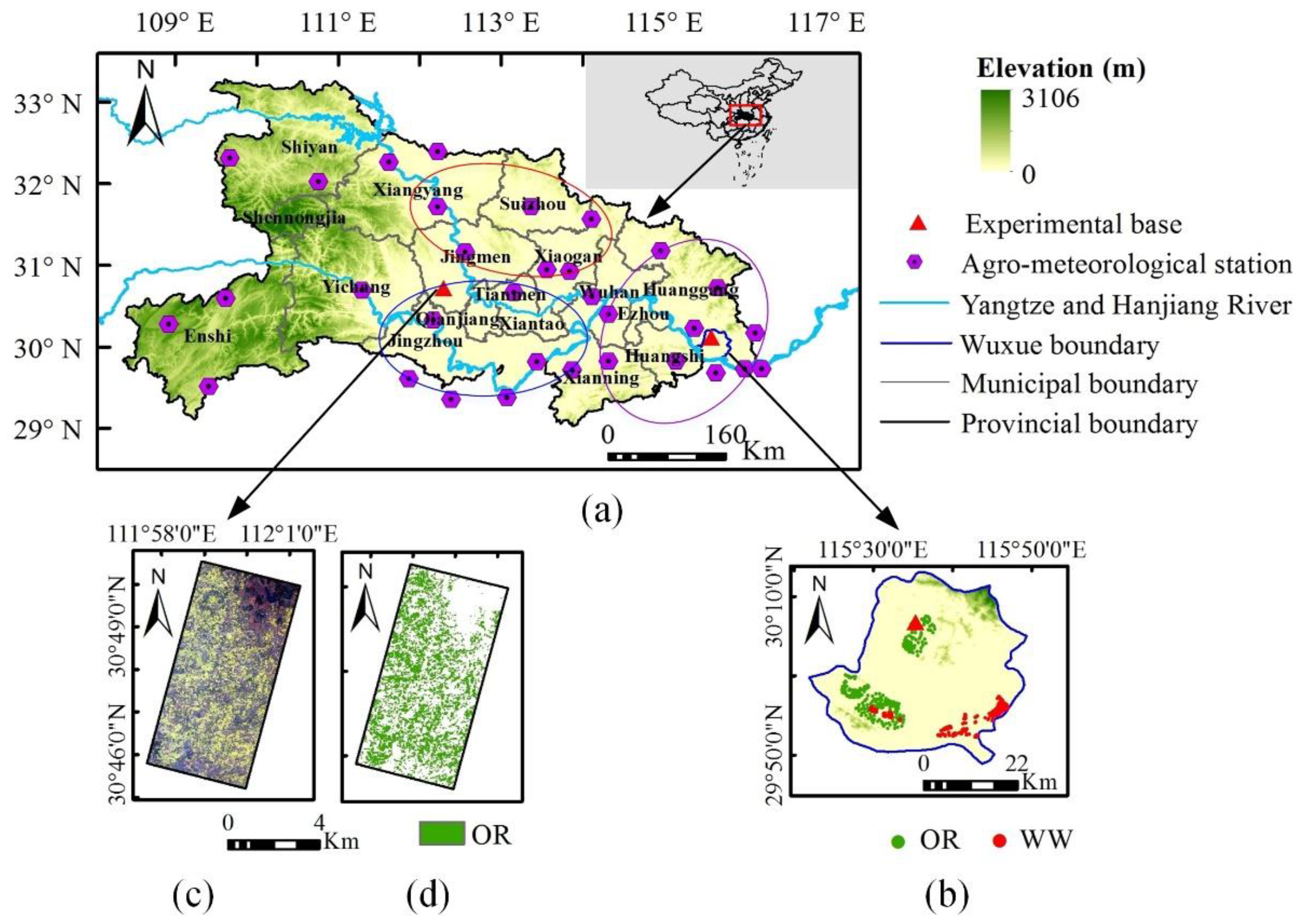
2.1. Study Area

Hubei Province (Figure 1a) is selected as the study area based on its status as a major Chinese agricultural province with the largest OR production in China. Hubei Province is located in Central China and extends from 108°21′ E to 116°07′ E in longitude and 29°05′ N to 33°20′ N in latitude, with the Yangtze and Hanjiang Rivers running through. The topography is characterized by an inclination overall going down from west to east with various landforms. The climate is humid subtropical and is largely controlled by the East Asian monsoon. The advantageous natural conditions promoted the excellent agricultural environment since ancient China. The crop species growing during winter growth season (from late September every year to mid-May in next year) in Hubei Province are OR and WW, based on the records of agro-meteorological stations. Hubei Province contributes one-sixth of the OR planting areas and products of China according to the statistical data from the China Statistical Yearbook. There are three OR producing areas with 80% planting areas and production in Hubei Province. The corresponding names for the different OR producing areas are: the Jianghan Plain (blue ellipse in Figure 1a, mainly containing Jinzhou, Xiantao, Tianmen, Qianjiang and part of Wuhan, Xiaogan, Yichang), the Eastern E Plain (E is a traditional abbreviation for Hubei Province, purple ellipse in Figure 1a, mainly containing Ezhou, Huanggang, Huangshi), and the Central-North E (red ellipse in Figure 1a, mainly containing Jinmen, Xiangyang and part of Xiaogan, Suizhou, Yichang). In fact, except for the high mountain area of Western Hubei Province, the whole mainland of Hubei Province is suitable for the growth of OR.

The OR experiment bases in Wuxue City and Shayang County of our research team were built in 2014 and 2016, respectively. Wuxue City (Figure 1b) is located in Eastern Hubei Province and famous for OR with “two low” (low erucic acid and low glucosinolate). Shayang County is located in Central Hubei Province and famous for OR with high production. OR is a traditional dominated crop species during winter growth season both in Wuxue City and Shayang County. During the OR planting and observing experiments, investigation of crop species in Wuxue City was conducted in 2015 and 2016, as well as in Shayang County in 2016.

2.2. Data Acquisition and Preprocessing

2.2.1. Remote Sensing Data

The remote sensing dataset used in this study is composed of sixty-six GF-1 WFV images, one GF-2 PMS image, and two RapidEye images. Among them, six GF-1 WFV images covering Wuxue City and representing continuous flowering stages of OR are used to learn and predict the parameter of the CSRA method. One GF-1 WFV, one GF-2 PMS, and two RapidEye images covering part of Shayang County in Jinmen are used to explore the robustness of the CSRA method. A summary of information regarding the application, sensor, acquisition date, number, coverage area, and phenology stage for these images are listed in

Table 1. The information of GF-1 WFV, GF-2 PMS, and RapidEye images used to build and verify the CSRA method. EFS, FBS, BFS, and EnFS in the table are the abbreviations of early flowering stage, full blooming stage, blossoming stage, and end flowering stage, respectively.

Application	Sensor	Acquisition Date	Number	Coverage	Phenology Stage
Building algorithm	GF-1 WFV	12 March 2015	1	Figure 1b	EFS
		17 March 2014	1		BFS
		25 March 2015	1		FBS
		28 March 2016	1		FBS
		2 April 2014	1		BFS
		10 April 2014	1		EnFS
Exploring robustness	GF-2 PMS	18 March 2016	1	Figure 1c	FBS
	RapidEye	18 March 2016	1		FBS
		4 April 2016	1		EnFS
	GF-1 WFV	28 March 2016	1		BFS

. The other GF-1 WFV images are used to produce OR maps of Hubei Province from 2014 to 2017, whose detailed information, like Table 1, are listed in

Table A1. The information of GF-1 WFV images used to produce OR maps of Hubei Province.

Application	Year	Acquisition Date	Number	Latitude/Longitude (°)	Coverage	Phenology Stage
Producing provincial OR maps using GF-1 WFV images	2014	03/17	4	28.9/113.9, 30.6/114.3, 32.3/114.8, 30.2/116.3	Eastern E	EFS
			1	29.7/109.9	Enshi City	FBS
		03/26	6	29.3/107.6, 31.0/108.0, 32.6/108.5, 30.6/109.9, 32.3/110.3,33.9/110.8	Western E	EnFS
			2	30.2/111.9, 31.8/112.4	Central E	BFS
		03/29	3	29.6/112.5, 31.3/112.9, 33.0/113.2	Central E	BFS
	2015	03/21	3	28.9/112.9, 30.6/113.3, 32.3/113.7	Central E	FBS
			4	33.0/109.3, 29.3/111.0, 30.9/111.4, 32.6/111.8	Western E	BFS
		03/25	1	31.3/111.4	Western E	BFS
			2	29.3/113.0, 30.9/113.4	Central E	FBS
			4	28.9/114.8, 30.6/115.2 32.3/115.7, 30.2/117.2	Eastern E	FBS
		03/13	2	29.6/108.9, 33.0/109.7	Western E	BFS
	2016	03/04	2	30.9/109.8, 30.6/111.6	Western E	EFS
		03/11	1	29.7/112.4	Central E	BFS
			1	29.3/114.9	Eastern E	EFS
		03/19	1	29.6/115.7	Eastern E	BFS
		03/28	3	29.6/110.9, 31.3/111.3, 33.0/111.7	Western E	EnFS
			3	29.3/113.0, 31.0/113.4, 32.6/113.8	Central E	BFS
			4	28.9/114.8, 30.6/115.2, 32.3/115.7, 30.2/117.2	Eastern E	FBS
		04/02	1	32.3/110.3	Eastern E	BFS
	2017	03/01	2	30.1/108.1, 33.4/109.2	Western E	EFS
		03/08	3	30.6/111.6, 30.2/113.6, 31.8/114.1	Central E	EFS
		03/28	2	33.0/109.3, 31.0/111.4	Western E	EnFS
			2	32.6/111.8, 32.3/113.8	Central E	FBS
		04/01	4	29.7/108.8, 31.4/109.1, 29.3/111.3, 31.0/111.7	Western E	EnFS
			2	31.8/115.5, 32.6/114.1	Eastern E	BFS

. The GF-1 WFV images are downloaded from the China Center for Resources Satellite Date and Application (CRESDA). The GF-2 PMS image is obtained from the Hubei Data and Application Center of High-Resolution Land-Observation Systems. The RapidEye images were bought by the research team. The series of GF imagery have the same spectral bands (blue, green, red, and near-infrared), and the detailed information can be browsed on the website of CRESDA. Compared with GF imagery, RapidEye imagery with 5 m spatial resolution and one-day temporal resolution has similar visible and near-infrared bands, but one more red edge band.

The preprocessing of GF-1 WFV images includes three protocols: geometric correction, radiometric calibration, and atmospheric correction. Geometric correction was conducted according to [37] with the assistance of ASTER GDEM V2 data. Radiometric calibration performs the conversion of image digital numbers to absolute at-sensor radiance. For each image, it was processed using the Environment for Visualizing Images (ENVI) 5.3 software (Harris Geospatial Solutions, Inc.: Broomfield, CO, USA) with the updating calibration parameters [42] published in CRESDA, obtained by a large number of calibration experiments in Chinese calibration fields. Atmospheric correction converts the radiance to reflectance. In this study, atmospheric correction was performed using the Fast Line-of-Sight Atmospheric Analysis of Spectral Hypercubes (FLAASH) model in ENVI and executed using the Interactive Data Language (IDL) (Harris Geospatial Solutions, Inc.: Redlands, CA, USA). Before correction, the cloud cover on the images were masked by visual interpretation. The related FLAASH parameters were obtained according to the acquisition time and imaging conditions.

The GF-2 PMS image is divided into the multispectral (MSS) image and panchromatic image. The preprocessing procedure of MSS image is same as GF-1 WFV images. The preprocessing of panchromatic image contains geometric correction and radiometric calibration. Geometric correction was conducted as same as MSS image. Radiometric calibration was conducted in ENVI by converting the digital numbers to the top of atmosphere reflectance. Afterwards, the Gram-Schmidt pan-sharpening method in ENVI was used to fuse the MSS and panchromatic images, which obtained a multispectral image with a 1 m resolution. The RapidEye images are L1C level products, which need preprocessing including geometric correction and atmospheric correction. The geometric correction and atmospheric correction procedures are same as GF-1 WFV images.

The fused GF-2 PMS image covering the overlap region among GF-2 PMS, RapidEye, and GF-1 WFV images was clipped (Figure 1c) and processed according to [25]. The processed result was further refined in ArcGIS Desktop 10.5 software (Environmental Systems Research Institute, Inc.: Broomfield, CO, USA) by visual interpretation based on the field investigation of Shayang County in 2016. Then, the reference OR map (Figure 1d) in this region was obtained by converting the modified boundaries of OR fields to raster data with 1 m resolution. At last, the reference OR map were resampled to 4 m, 5 m, and 16 m resolution using pixel aggregate resampling method, which were used to assess the accuracy of CSRA-derived OR results on GF-2 PMS MSS, RapidEye, and GF-1 WFV images, respectively.

2.2.2. Ancillary Data

The ASTER GDEM V2 data, used for the geometric correction of satellite images, is a global digital elevation model (DEM) with 30 m resolution. The V2 data within the range of Hubei Province are downloaded from the Geospatial Data Cloud.

The phenology of OR in this study is obtained from the agro-meteorological stations in and near Hubei Province (purple hexagon in Figure 1a). The flowering period of OR divides into four stages: EFS (from the beginning of flowering to the flowers proportion less than 25% in the field), FBS (flowers proportion is more than 75%), BFS (flowers proportion is between 25% and 75%), and EnFS (flowers proportion is less than 25% and close to pod stage). Thus, a complete flowering period of OR are composed of EFS, BFS, FBS, BFS, and EnFS, successively. The flowering period in Hubei Province appears as an obvious gap in Yichang City. The left region of Yichang belonging to the upper reaches of the Yangtze River with a flowering period from early March to late March, whereas the right region of Yichang belongs to the middle reaches of the Yangtze River with a flowering period from mid-March to early April. The date gap between the two regions is nearly ten days.

The statistical planting areas of OR in Hubei Province from 2014 to 2016 (the data of 2017 will be published at the end of 2018) at provincial and municipal levels are used to validate the CSRA-derived OR planting maps. The statistical data are downloaded from the National Statistical Bureau of China and the Hubei Statistical Bureau.

Google Earth (GE) releases free images in high spatial resolution that may provide some potential for regional land use/cover mapping. Studies regarding land cover classification and validation using GE images achieved good effects [43,44]. Thus, we employed the GE images to assist with the validation of OR classification results in this study. Historical GE images with 1 m resolution at FBS in part of Qianjiang City in 2015 (Figure 2a) and Wuxue City in 2016 (Figure 2c) were downloaded to validate the provincial OR planting maps. Registration of the GE images was performed based on GF-1 WFV images firstly, then object-oriented classification was conducted in eCognition 8.6 software to extract OR as the local reference OR map. The multi-resolution segmentation parameters for scale, shape, and compactness used in GE image processing were 30, 0.2, and 0.5, respectively. The nearest neighbor method classification method was used.

2.2.3. Samples Collection

The land cover types in winter growth season of Hubei Province contain OR, WW, forest land, built-up land, water body, and bare land. Among them, crop species (OR and WW) and forest land make up the vegetation types. Built-up land, water bodies, and bare land compose non-vegetation types. In this study, sample collection for these land cover types is focused on Wuxue City, which is divided in two ways: field survey and visual interpretation. The field investigation with contents of the crop (OR and WW) was conducted in three experimental regions around Wuxue City in 2015 and 2016. The sampling method in each region was a simple random sample. The sample points (Figure 1b) of OR and WW were 2292 and 1669, respectively. Other land cover types, including forest land, built-up land, water bodies, and bare land, were collected on GF-1 WFV images by visual interpretation. These land cover types show obvious visual differences among each other, as well as when compared with crop species during the whole flowering period. The region of interest tool in ENVI was applied to collect samples of these land cover types with simple random sampling method. The sample points were evenly distributed over the entire image, and the number of forest land, built-up land, water bodeis, and bare land were 1662, 1922, 1810, and 621, respectively. For accuracy assessment of CSRA-derived results of six GF-1 WFV images of Wuxue City, the sample points of each type were divided into training samples and validation samples. Noticeably, the CSRA-derived results are a map with two classes (OR and NOR). Thus, WW, forest land, built-up land, water bodies, and bare land of the validation sample were merged into the NOR class. As a result, the pixel number of training samples of OR, WW, forest land, built-up land, water bodies, and bare land were 1278, 1069, 1512, 1802, 1710, and 577, respectively. The pixel number of the validation sample of OR and NOR were 1044 and 1014, respectively.

2.3. Mapping Approach of Oilseed Rape

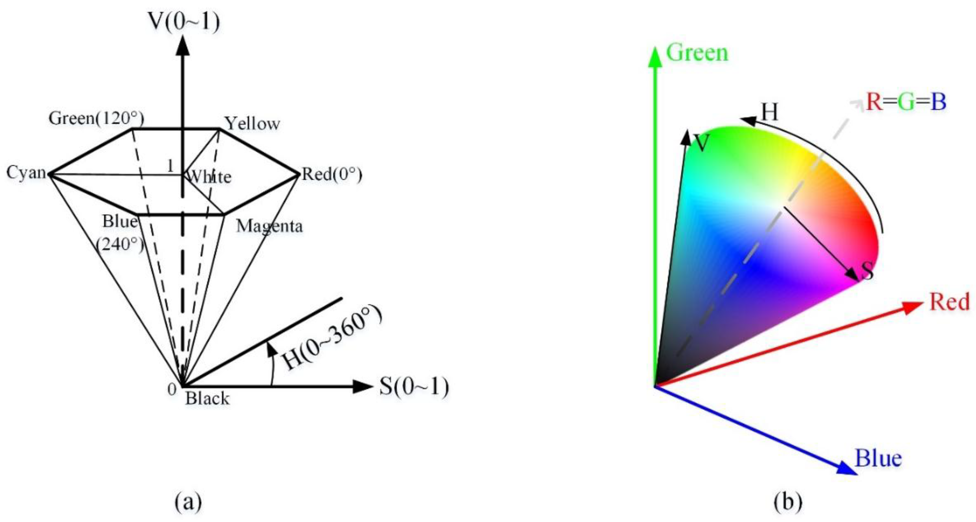
2.3.1. NDVI Model, HSV Transformation, and Normalization

VIs are quantitative measurements indicating the vigor of vegetation. The interest of these indices lies in their usefulness in the interpretation of remote sensing images and the improvement of classifications [45]. Among them, NDVI is sensitive to the presence of green vegetation, the prediction of agricultural crops, and precipitation in semi-arid areas [45]. In this study, NDVI is used to analyze the difference between vegetation and non-vegetation types. Equation (1) is the formula for calculating NDVI:

$$\mathrm{NDVI}=\frac{NIR-\mathrm{R}}{NIR+\mathrm{R}}$$

(1)

where $NIR,\mathrm{R}$ represent the reflectance at near-infrared and red bands, respectively.

Case studies have shown that color features are effective for crop discrimination [26,27]. Compared with the RGB color space, the HSV color space has better performance to some extent in terms of decoupling chromaticity and luminance [28,29,30]. Figure 3a describes the meaning of HSV components: H is defined as an angle between 0° and 360° representing a pure color (e.g., pure yellow, orange, or red, etc.); S refers to how much a pure color is diluted with white light; and V is the brightness of the color. The value of both S and V are between 0 and 1. Figure 3b shows the geometric relationship between the RGB and HSV systems. The transformation from the RGB color space to the HSV color space keeps the “black” vertex fixed at the origin, and the diagonal of the RGB color cube (named achromatic axis) is vertical so that the red, green, and blue axes are symmetrically arranged around the vertical axis that corresponds to the V axis of the HSV space [29]. Equation (2) is used to perform the HSV transformation, which is a standardized transformation and a faster version as it does not contain any trigonometric functions or other functions requiring high-performance computation [29]. Thus, it supports the efficiency of pixel-level calculation to a large extent of satellite imagery.

$$\{\begin{array}{c}\mathrm{V}=\max \left(\mathrm{R},\mathrm{G},\mathrm{B}\right)\\ \mathrm{S}=\frac{\mathrm{V}-\min \left(\mathrm{R},\mathrm{G},\mathrm{B}\right)}{\mathrm{V}}\\ \mathrm{H}=\{\begin{array}{c}\begin{array}{c}0,\mathrm{if}\mathrm{V}=\min \left(\mathrm{R},\mathrm{G},\mathrm{B}\right)\\ \left(60°*\frac{\mathrm{G}-\mathrm{B}}{\mathrm{V}-\min \left(\mathrm{R},\mathrm{G},\mathrm{B}\right)}+360°\right)\mathrm{mod}360°,\mathrm{if}\mathrm{V}=\mathrm{R}\end{array}\\ \begin{array}{c}60°*\frac{\mathrm{B}-\mathrm{R}}{\mathrm{V}-\min \left(\mathrm{R},\mathrm{G},\mathrm{B}\right)}+120°,\mathrm{if}\mathrm{V}=\mathrm{G}\\ 60°*\frac{\mathrm{R}-\mathrm{G}}{\mathrm{V}-\min \left(\mathrm{R},\mathrm{G},\mathrm{B}\right)}+240°,\mathrm{if}\mathrm{V}=\mathrm{B}\end{array}\end{array}\end{array}$$

(2)

where $R,G,B$ represent the reflectance at red, green, and blue bands, respectively. As the perceived color is determined by the shape of the (corrected) spectral reflectance, changes of HSV components are equivalent to the changes in land cover types. Especially, the change from one color to another color is interpreted as a land cover change [29]. Thus, it is possible to associate a land cover type to a range of H, as well as the auxiliary decision by S and V.

The value of NDVI is between −1 and 1. The reflectance at blue, green, red, and near-infrared bands, S, and V are all between 0 and 1, whereas H is between 0 and 360. Moreover, H and V will be used to establish new indicators for extracting OR from other crop species. Thus, for further analysis, normalization for H is needed. And equation (3) is used to normalize H between 0 and 1:

$${\mathrm{H}}_{\mathrm{norm}}=\frac{\mathrm{H}-\min \left(\mathrm{H}\right)}{\max \left(\mathrm{H}\right)-\min \left(\mathrm{H}\right)}$$

(3)

where $\mathrm{H}$ means variable H with a value between 0 and 360, ${\mathrm{H}}_{\mathrm{norm}}$ means the normalized variable H with a value between 0 and 1.

2.3.2. Spectral and Color Characteristics of Land Cover Types on GF-1 WFV Images in Wuxue City

All the satellite images are conducted to execute the NDVI calculation, HSV transformation, and normalization. Then, the spectral feature (reflectance at each band, NDVI) and color feature (${\mathrm{H}}_{\mathrm{norm}}$, S, and V) values of the training sample on GF-1 WFV images of Wuxue City are exported. Afterwards, the average and standard deviation values of each land cover type are calculated to analyze the multi-temporal features. Finally, we found that NDVI, reflectance at near-infrared band (NIR), ${\mathrm{H}}_{\mathrm{norm}}$, and V are sensitive to separate OR from other land cover types based on stepwise analysis. Figure 4 shows the multi-temporal features regarding spectral and color features applied to CSRA method.

The multi-temporal NDVI in Figure 4a reveal that the NDVI values of vegetation types (OR, WW, and forest land) are always much larger than non-vegetation types (built-up land, water body, and bare land) even through the NDVI values of each type change over time. The rationale is that all these images are in plant growth season that vegetation species have large biomass, which can be reflected by NDVI. Thus, NDVI is used to separate non-vegetation types from vegetation types firstly.

Afterwards, we found there is a large difference in NIR among the vegetation types. As shown in Figure 4b, the NIR of crop types (OR and WW) are much larger than non-crop types at six flowering stages. The reason is that the crop species growing in Southern China in this period are in the reproductive growth stage, whose canopy, with dense leaf blade strongly reflecting the solar energy, while the forest type in this period are in the nutritional growth stage, with leaf blades starting growth. Thus, the reflectance in the near-infrared band of the forest type are small. Therefore, NIR is used to distinguish crop and non-crop types.

In the rest of the crop types, the reflectance at each band between OR and WW of images at EFS and EnFS have large similarity, caused by the flower proportion influencing the reflectance, as described in Section 1. However, we notice the difference between OR and WW at EFS and EnFS are still large in the HSV color space. In Figure 4c, ${\mathrm{H}}_{\mathrm{norm}}$ of WW is larger than OR at each stage, whereas V of WW is slightly smaller than OR. Thus, the ratio of V and ${\mathrm{H}}_{\mathrm{norm}}$ can be used to enlarge this difference. Additionally, the threshold of the ratio of V and ${\mathrm{H}}_{\mathrm{norm}}$ can be used to classify OR and WW. However, the differences at each flowering stage are not uniform, which would cause varying thresholds at each flowering stage and additional mixing (Figure 4d) when analyzing all the samples together. This mix can be solved by dividing the ${\mathrm{H}}_{\mathrm{norm}}$-V space into three parts (part 1: V ≥ 0.07 and ${\mathrm{H}}_{\mathrm{norm}}$ ≤ 0.25; part 2: V ≥ 0.12 and 0.25 < ${\mathrm{H}}_{\mathrm{norm}}$ ≤ 0.42; and part 3: 0.07 ≤ V < 0.12 and 0.25 < ${\mathrm{H}}_{\mathrm{norm}}$ ≤ 0.42). The separability of OR and WW in each part is large. Thus, the ratio of V and ${\mathrm{H}}_{\mathrm{norm}}$, named RRCI (ratio oilseed rape colorimetric index), is defined as Equation (4) to classify OR and WW in this study:

$$\mathrm{RRCI}=\frac{\mathrm{V}}{{\mathrm{H}}_{\mathrm{norm}}}$$

(4)

2.3.3. Workflow of Extracting Oilseed Rape

The workflow of applying CSRA method on remote sensing data to extract OR in this study is shown in Figure 5. It includes:

(1)

Data collecting and preprocessing, which has been introduced in Section 2.2.

(2)

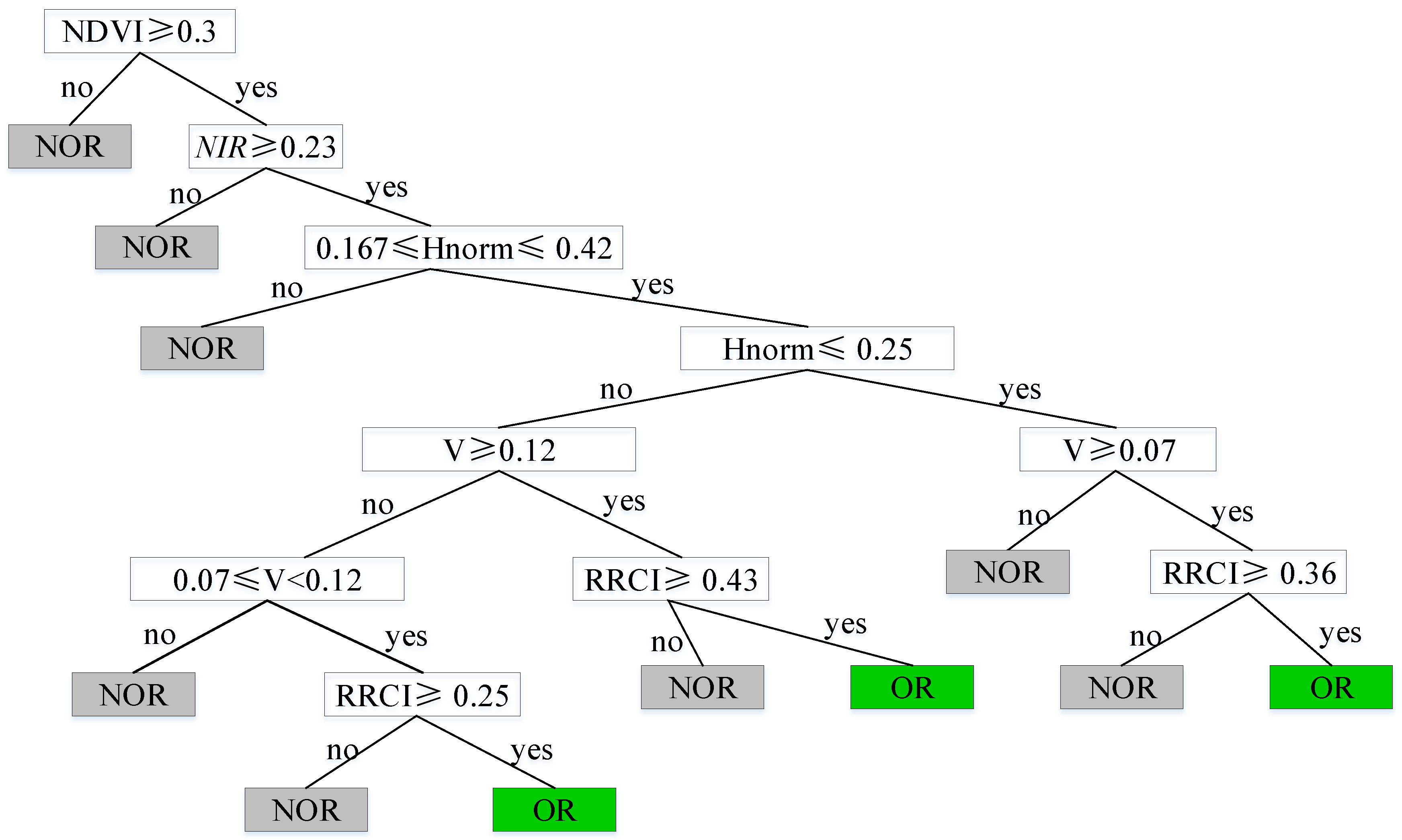
Developing the CSRA method based on GF-1 WFV-derived samples of Wuxue City. Section 2.3.2 has introduced the general idea of CSRA, which is a stepwise exclusive approach to achieve the goal of extracting OR. NDVI, NIR, and RRCI are successively used to separate vegetation from non-vegetation types, crop from non-crop types, and OR from WW. The threshold value in each step is obtained by the histogram thresholding method, which is the refined overlap point beyond two groups [3]. Finally, the CSRA approach is performed to define the classification rules of the decision tree as its effectiveness and efficiency having been proved in the field of remote sensing classification [5,46]. The CSRA method is executed using IDL. The acquisition of threshold values and detailed DT of the CSRA method will be reported in Section 3.1.

(3)

Applying the CSRA method on remote sensing images to produce OR planting maps automatically. The OR maps includes: six GF-1 WFV-derived OR planting maps of Wuxue City, abbreviated as Result 1; GF-1 WFV-derived OR planting maps of Hubei Province from 2014 to 2017, abbreviated as Result 2; one GF-1 WFV-derived, one GF-2 PMS MSS-derived, and two RapidEye-derived OR planting maps of the overlap region of these four images, abbreviated as Result 3.

(4)

Validating the OR maps. The detailed validation contents regarding validating methods and dataset will be introduced in Section 2.3.4.

2.3.4. Results Validation

Result 1 and Result 3 are validated using the confusion matrix. Overall accuracy, kappa coefficient, user accuracy, and producer accuracy are used to assess the accuracy of the CSRA method. The validating samples of Result 1 are the validation samples introduced in Section 2.2.3. The validating sample of Result 3 are the OR and NOR pixels of the reference OR map in that region (Figure 1d).

The validation for Result 2 includes: local spatial consistency validation and area comparison against agricultural census data at provincial and municipal levels. The local spatial consistency is validated using confusion matrix basing on the GE image-derived OR reference maps (Figure 2b,d). The provincial level area comparison is validated using relative error between the CSRA-derived OR planting areas and the statistical areas of agricultural census data. Equation (5) is the formula for the relative error:

$$\mathrm{RE}=\left(\mathrm{Extraction}-\mathrm{Reference}\right)/\mathrm{Reference}\times 100\%$$

(5)

where $\mathrm{RE}$ means the relative error, $\mathrm{Extraction}$ means the estimated areas, and $\mathrm{Reference}$ means the statistical areas. The municipal level area comparison is validated using decision coefficients (R²) between the CSRA-derived OR planting areas and the statistical areas of agricultural census data.

3. Results

3.1. Classification Rules of the CSRA Method

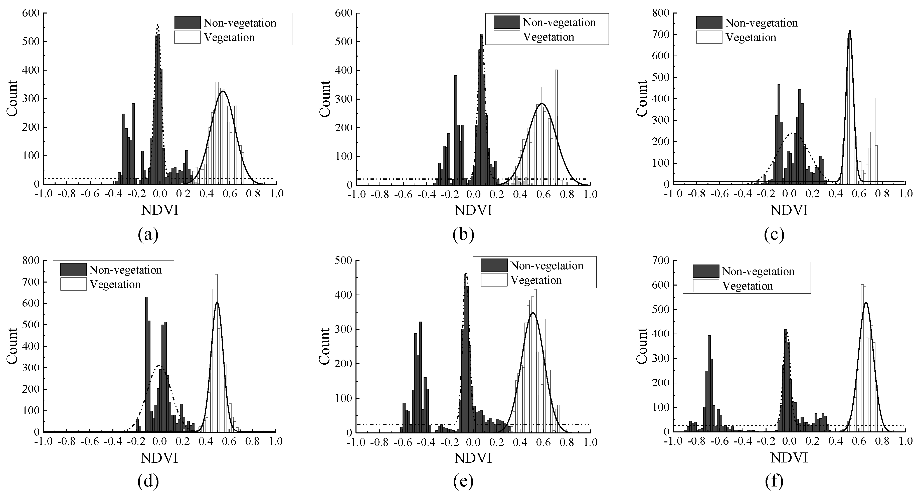
(1)

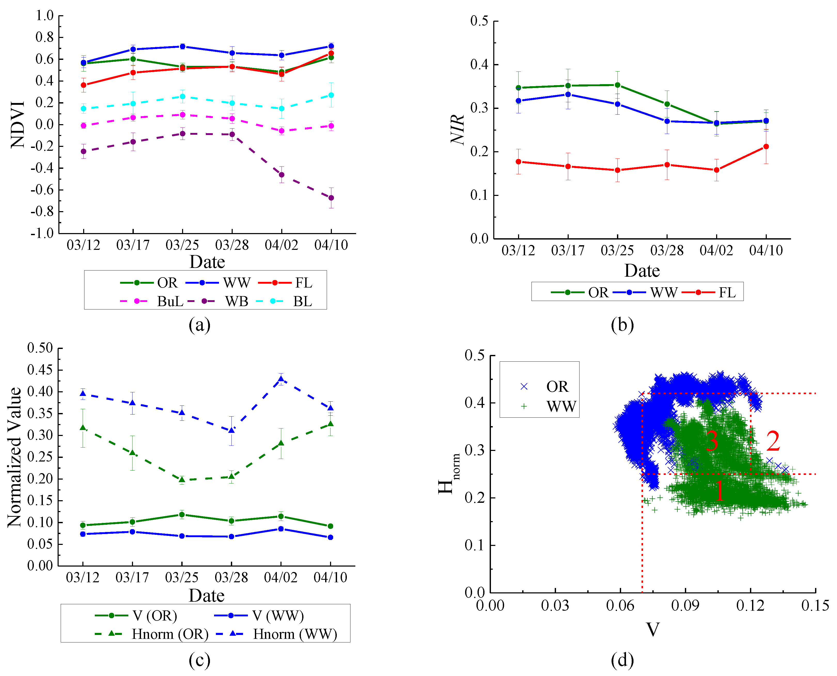
Vegetation and non-vegetation types. Figure 6a–f shows the histogram results of NDVI between vegetation and non-vegetation types corresponding to 03/12, 03/17, 03/25, 03/28, 04/02, and 04/10, respectively. The threshold of NDVI for classifying vegetation from non-vegetation types is 0.3 at each flowering stage. Thus, the first step of the CSRA method is classifying vegetation pixels from non-vegetation pixels using the rule: NDVI ≥ 0.3.

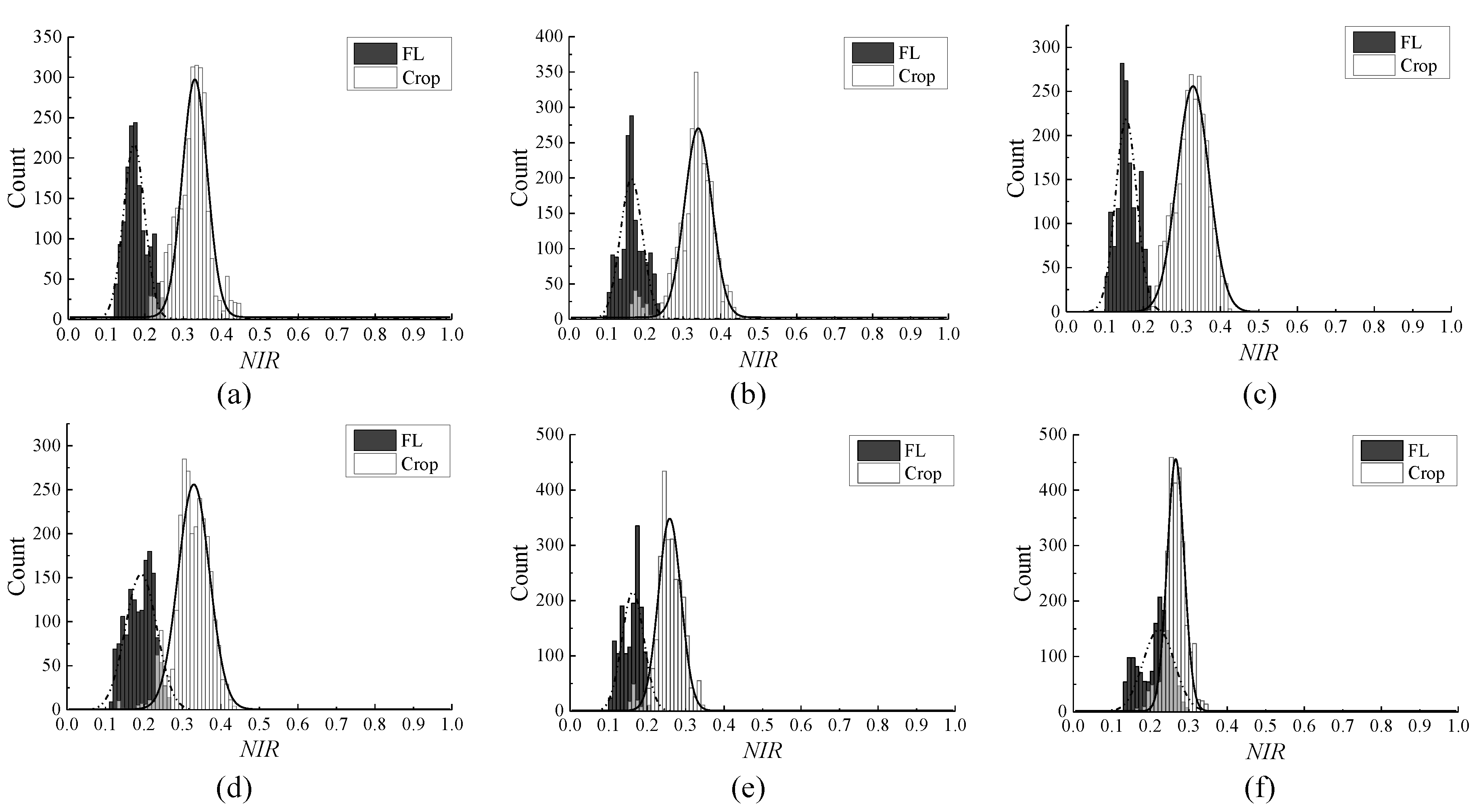
(2)

Crop and non-crop types. Figure 7, regarding the histogram groups of NIR for crop and forest land, reveals that NIR is useful to distinguish them with a threshold of 0.23. Figure 7f shows some overlap with part of the FL samples having NIR values larger than 0.23, which is caused by the beginning of tree’s nutritional growth stage since early April every year in Yangtze River Basin, China. These samples were gathered and analyzed in the next step. Thus, the second step of the CSRA method is separating the crop pixels from FL using the rule: NIR ≥ 0.23.

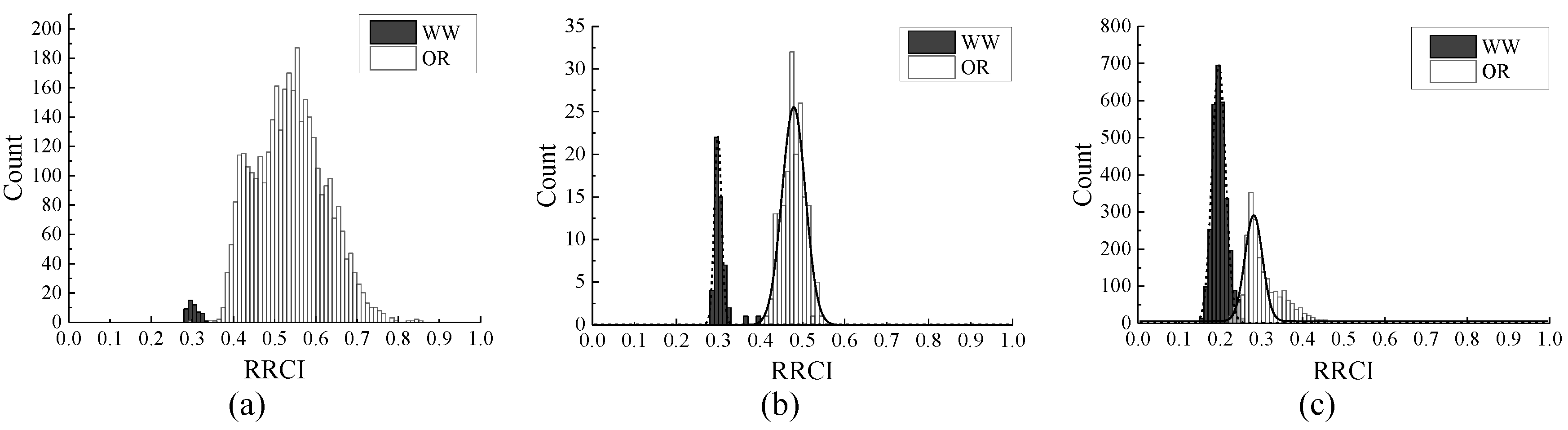
(3)

OR and WW. Figure 8 shows the performance of RRCI for distinguishing OR and WW, which has good separability in each part of the ${\mathrm{H}}_{\mathrm{norm}}$-V space. The thresholds for parts 1–3 are 0.36, 0.43, and 0.25, respectively. In addition, the remaining forest land samples in step (2) can be divided into two groups: the first group with V values smaller than 0.07 and the second group located in part 3 of the ${\mathrm{H}}_{\mathrm{norm}}$-V space. The RRCI values of the second group are all smaller than 0.2. Thus, the FL samples with NIR values larger than 0.23 have no confusion with OR. Therefore, the third step of the CSRA method is separating OR from WW using the rules: RRCI ≥ 0.36 when V ≥ 0.07 and $H_{norm}$ ≤ 0.25; RRCI ≥ 0.43 when V ≥ 0.12 and 0.25 < $H_{norm}$ ≤ 0.42; and RRCI ≥ 0.25 when 0.07 ≤ V < 0.12 and 0.25 < $H_{norm}$ ≤ 0.42.

According to [30], the H value of vegetation types is between 60 and 180 because of the “green peak” of reflectance for vegetation types. Thus, the rules of $H_{norm}$ ≥ 0.167 is needed. Finally, all the rules are used to construct the decision tree of the CSRA method for extracting OR, which is shown in Figure 9.

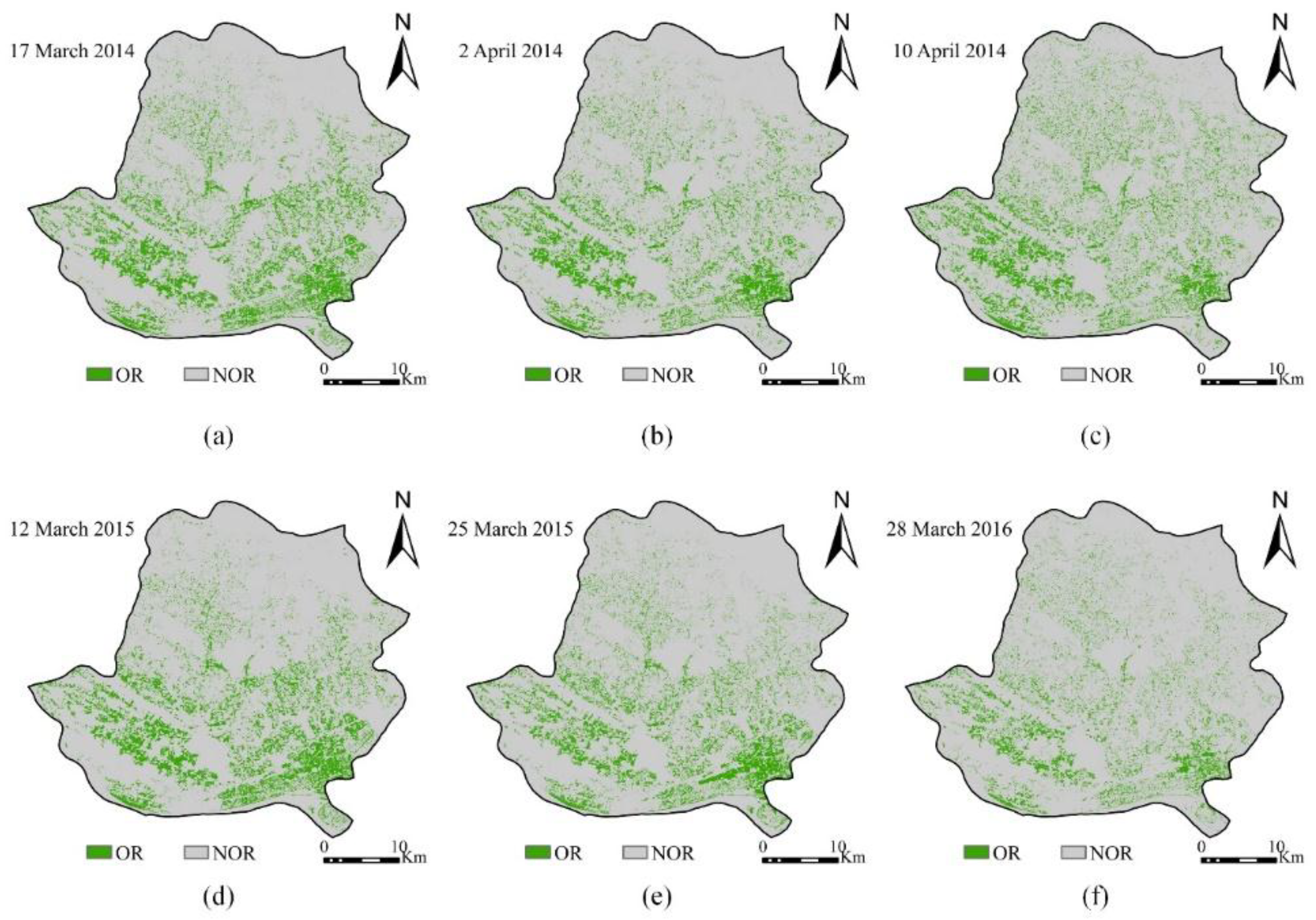
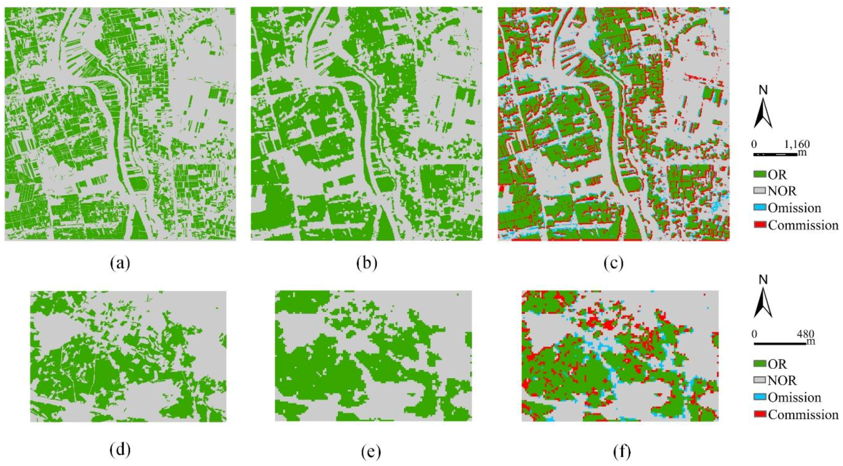
3.2. Mapping Oilseed Rape in Wuxue City Using the CSRA Method and Accuracy Assessment

The presented CSRA approach is firstly applied to generate the spatial distributions of OR in Wuxue City using the six GF-1 WFV images. Figure 10a–f, ranged chronologically for a more intuitive contrast, are the results corresponding to 03/17, 04/02, 04/10, 03/12, 03/25, and 03/28, respectively. As shown in Figure 10, OR is mainly planted in Southern Wuxue City because of the excellent growth conditions composing of the running Yangtze River and the flat topography, while the Northern part is mainly scattered and small fields due to hilly terrain. Figure 10 also shows that the planting areas of OR in Wuxue City from 2014 to 2015 are basically stable, whereas from 2015 to 2016 there appears to be an obvious decrease. In fact, the planting areas of OR in Wuxue City from 2014 to 2016 are 30, 28.96, and 20.7 Kha, respectively. Thus, the tendency reflecting OR planting areas are coincidental between the CSRA-derived results and the agricultural census data.

Table 2. Accuracy assessment for CSRA-derived oilseed rape maps in Wuxue City.

Accuracy	03/12	03/17	03/25	03/28	04/02	04/10
PA (%)	93.77	91.09	98.28	98.47	98.37	96.36
UA (%)	86.48	88.47	94.21	93.62	89.23	85.40
OA (%)	89.41	89.46	96.06	95.82	93.15	89.80
kappa	0.79	0.79	0.92	0.92	0.86	0.80

PA: producer accuracy; UA: user accuracy; OA: overall accuracy.

lists the accuracy assessment results of these OR maps. The accuracy results have an increase from EFS to FBS whereas a decrease from FBS to EnFS. The rationale is that the RRCI separability between OR and other crop species also have an increase from EFS to FBS whereas there is a decrease from FBS to EnFS, since the color features are derived and affected by the reflectance at blue, green, and red bands. The overall accuracy of all results are larger than 89%, as well as kappa larger than 0.79. The producer accuracy of all results are larger than 91%. The user accuracy at EFS and EnFS are relatively worse because of the strong confusion between OR and WW at these phenology stages. However, the accuracy values are still larger than 85%. Thus, these accuracy results show good performance of the CSRA method on extracting OR. The results of Wuxue City demonstrated the effectiveness of the CSRA method on OR extracting at each flowering stages, which means the phenology problem is solved by the CSRA method.

3.3. Producing and Validating the Provincial Oilseed Rape Planting Maps

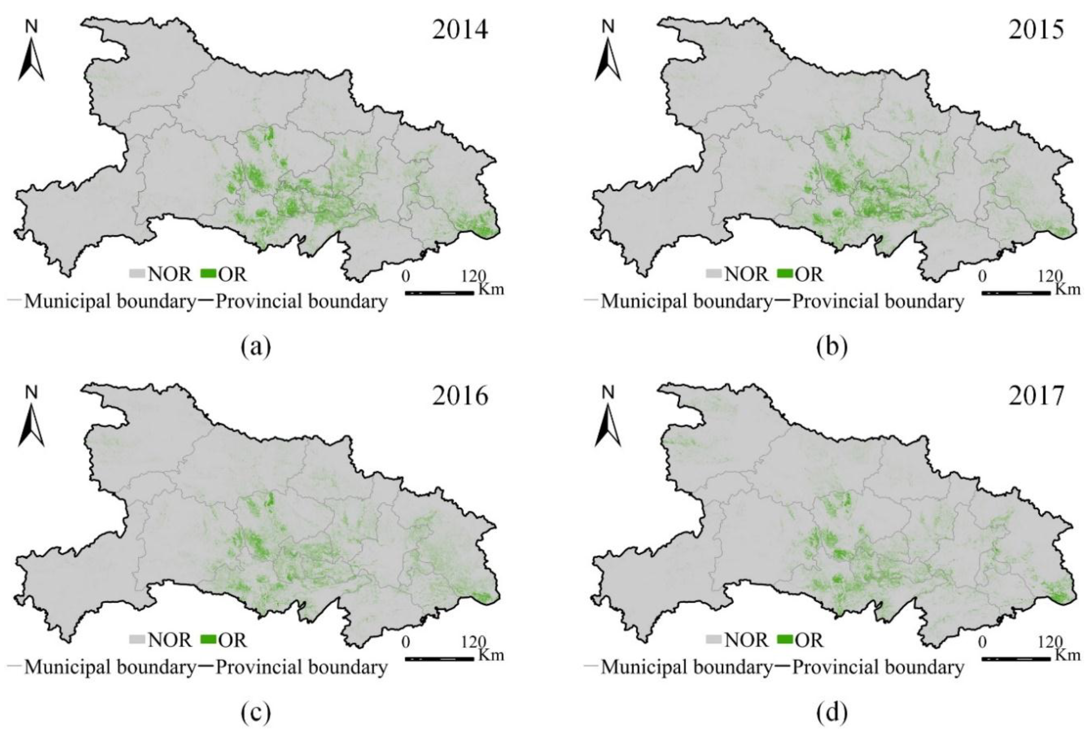
3.3.1. Spatial Distribution of Oilseed Rape in Hubei Province and Local Accuracy Assessment

Figure 11 shows the spatial distribution of OR in Hubei Province derived from GF-1 WFV images using the CSRA method. From 2014 to 2017, OR agriculture are concentrated in major regions near the Yangtze River and the Hanjiang River, whereas it occurs more sporadically in the western portion of the study area. The increased complexity of the topography in Western Hubei Province restricts the size of OR fields with most of the OR agriculture occurring in smaller river valleys or on terraced slopes. The largest planting area of OR are successively Jinzhou, Huanggang, and Jinmen, which corresponds to the major municipal City of Jianghan Plain, Eastern E Plain, and Central-North E mentioned in Section 2.1. The planting areas of OR estimated by the CSRA method from 2014 to 2017 are 1028.37, 1003.39, 965.23, and 811.83 Kha, respectively. It has nearly no changes from 2014 to 2015, whereas there are successive decreases in 2016 and 2017. The decrease in 2016 mainly occurs in Tianmen, Xiantao, and Qianjiang. Cloud cover in Xiantao, Huangshi, and Jinmen in 2017 affect the accuracy of the results. However, Huanggang, Tianmen, and Suizhou have obviously decreased, except for those regions. The reason for the decrease are the increased planting costs and reduced market returns according to the agricultural announcement of the Hubei Provincial Department of Agriculture.

The spatial matching of the OR planting maps is very important for practical applications. Local GE images are used to validate the spatial consistency of GF-1 WFV derived OR maps by the CSRA method. Figure 12a,d are the GE image-derived OR maps in part of Qianjiang City in 2015 and Wuxue City in 2016, respectively. Figure 12b,e shows the corresponding GF-1 WFV-derived OR maps of Figure 12a,d, respectively. The results show that the GF-1 WFV-derived OR maps have same spatial distribution compared with the GE image-derived OR maps. However, the GF-1 WFV-derived results have larger planting areas than the GE image-derived results due to the difference in spatial resolution. Furthermore, spatial analysis is conducted between the GF-1 WFV-derived and the resampled GE image-derived OR maps (Figure 12c,f). Additionally, the confusion matrix (

Table 3. Confusion matrix of local accuracy assessment using Google Earth images.

Figure 12c				Figure 12f
Class	OR	NOR	PA (%)	Class	OR	NOR	PA (%)
OR	48371	5731	89.41	OR	3307	421	88.71
NOR	10405	77997	88.23	NOR	960	4713	83.08
UA (%)	82.30	93.16		UA (%)	77.50	91.80
OA (%)	88.68 (kappa = 0.76)			OA (%)	85.31 (kappa = 0.70)

PA: producer accuracy; UA: user accuracy; OA: overall accuracy.

) is performed to assess the accuracy using the spatial analysis results. The overall accuracy of Figure 12c is 88.68%, and Figure 12f is 85.31%. The user accuracy of GF-1 WFV-derived results are relatively low. The first reason for that is the difference of spatial resolution. For example, the GE image-derived OR maps can clearly extract OR fields and field borders, whereas the GF-1 WFV-derived results cannot distinguish fields borders from fields. The difficulty for co-registering GE images with GF-1 WFV images is the second reason. Even in this situation, larger than 85% overall accuracy and nearly 90% producer accuracy still proves the CSRA-derived OR maps using GF-1 WFV images obtain high spatial consistency when compared with GE image-derived reference OR maps.

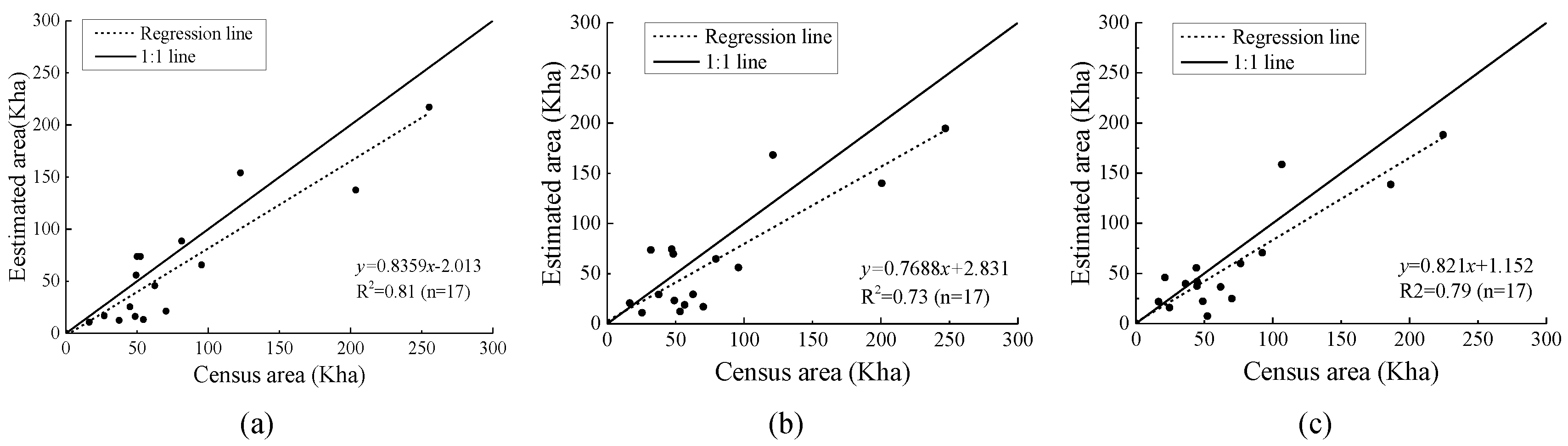
3.3.2. Comparison of the Estimated Oilseed Rape Planting Areas with Agricultural Census Data

The comparison results (

Table 4. Comparison of oilseed rape planting areas derived using the CSRA algorithm and from the agricultural census data.

Region	Year	CA (Kha)	EA (Kha)	RE (%)
Hubei Province	2014	1248.7	1028.37	−17.65
	2015	1232.13	1003.39	−18.57
	2016	1150.43	965.23	−16.01
	2017		811.83

Note: CA: census areas; EA: estimated areas.

) between the GF-1 WFV-estimated OR planting areas and the agricultural census data at the provincial level confirm good accuracy. The absolute errors of the extracted annual total OR areas are less than 20%. The total OR planting areas of Jianghan Plain, Eastern E plain and Central-North E have provincial proportions of 78.47%, 76.24%, 77.67%, and 73.41% from 2014 to 2017, respectively, which are extremely well matched with the actual proportion of 80% published by the Hubei Provincial Department of Agriculture. The tendency of both estimated and statistical OR planting areas confirm a decrease occurring in 2016, which had the same conclusion with the analysis of Section 3.3.1.

Furthermore, municipal-level validation of the OR planting areas extraction results is performed. The comparison results between the GF-1 WFV-estimated OR planting areas and the census data are shown in Figure 13. The solid line in the plot is the 1:1 line. The points in the plot are clustered near the 1:1 line, indicating that the GF-1 WFV-derived areas of OR is well correlated with the agricultural census data at the municipal level. The R² for 2014, 2015, and 2016 are 0.81, 0.73, and 0.76, respectively, which are all significant at the level of p < 0.01 (n = 17). The largest estimated mistakes of OR planting areas always appear in Shiyan, Enshi, and Xianning. One reason for that is the poor data availability caused by long-term cloud cover. Another reason is the omission error caused by the small fields in these mountain regions. The small fields are often processed as mixed pixels on GF-1 WFV images with uncertain reflectance. Generally, the GF-1 WFV-derived OR planting areas had good accuracy when comparing with agricultural census data. Furthermore, the tendency of the spatial distribution and local spatial consistency assessed in Section 3.3.1. also show a good effect. On the other hand, it is a time-consuming and labor-intensive task to implement a large-scale regional survey of OR planting areas and to obtain an annual spatial distribution map. Therefore, basing on the good spatial consistency, as well as the strong relationship between the GF-1 WFV-derived results and the agricultural census data from 2014 to 2017, the CSRA method can help to provide accurate OR area estimation and spatial distribution at the large-regional scale.

3.4. Robustness Validation of the CSRA Method

Section 3.2 and Section 3.3 have proved the effectiveness of the CSRA method on GF-1 WFV images. In this part, the CSRA method is used to explore its robustness using the GF-2 PMS MSS and RapidEye images. Figure 14 shows the spatial analysis results between the CSRA-derived OR maps and the reference OR map (Figure 1d). Figure 14a–d shows the results of the GF-2 PMS MSS image on 18 March 2016, the RapidEye images on 18 March 2016 (03/18) and 4 April 2016 (04/04), and the GF-1 WFV image on 28 March 2016, respectively. Figure 14e–h shows the corresponding results of the black rectanglar regions in Figure 14a–d.

Table 5. Accuracy assessment for the CSRA-derived oilseed rape maps of GF-2 PMS MSS, RapidEye, and GF-1 WFV images in part of Shayang County.

Accuracy	GF-2 PMS MSS	RapidEye (03/18)	RapidEye (04/04)	GF-1 WFV
PA (%)	99.78	98.11	92.66	88.93
UA (%)	90.85	85.67	84.85	80.35
OA (%)	96.48	93.72	91.80	88.72
kappa	0.92	0.87	0.82	0.76

PA: producer accuracy; UA: user accuracy; OA: overall accuracy

shows the accuracy assessment results of these OR maps. These results show: (1) the GF-2 PMS MSS-derived result has the best spatial consistency, whereas GF-1 WFV has the worst; (2) all the misclassified pixels (omission and commission pixels) are distributed in the boundary area of OR fields; and (3) the RapidEye (04/04)-derived OR map has more omission and commission errors compared with the RapidEye (03/18)-derived result. The difference of the spatial consistency results between GF-2 PMS and GF-1 WFV are mainly caused by spatial resolution, which has been analyzed in Section 3.3. The GF-2 PMS MSS-derived OR map achieved 96.48% overall accuracy, which shows excellent spatial consistency with the reference OR map, and the GF-1 WFV-derived OR map also achieves 88.72% overall accuracy. The difference between the two RapidEye-derived results is caused by the acquisition date of the images. The images on 03/18 and 04/04 are at the FBS and EnFS, respectively, in which differences objectively exist when extracting OR. However, the accuracy assessment results (Table 5) show these differences are not large. The RapidEye-derived OR map on 04/04 achieves 91.8% overall accuracy, as well as 93.72% on 03/18. Both of these two images have good spatial consistency with the reference OR map. Thus, these results prove the good robustness of the CSRA method to some extent.

4. Discussion

4.1. Comparison with Previous Works

Table 6. Comparison of the existing OR extracting approaches using multispectral images.

Reference	Objective	Extracting Approach for OR	Study Area	Phenology Stage
[11]	Assessing freeze injury of OR	MDC	Five counties near Hefei City, China	FBS
[16]	Extracting OR planting areas	MLC, MDC, ISODATE	Shou County, China	FBS
[17]	Extracting OR planting area	SVM, MLC, ARTMAP	5 km × 5 km area in Haiyan country, China	FBS
[19]	Extracting OR	DVI	Luoping County, China	FBS
[20,21]	Classifying OR from WW	NDVI	Hubei Province, China	FBS and BFS
[23]	Crop classification	MDC	Jianli County, China	FBS
[22]	Identifying OR	MDC and GIS analysis	Northern Germany	Flowering
[24]	Classifying cruciferous weed from WW	SVM, MLC, G, NIR, B/G, NDVI, DVI, RVI	15.76 km × 6.47 km area in Southern Spain	Flowering
[3]	Estimating vegetation and flower fraction	NGVI	Wuxue experiment base in Section 2.1	BFS
[25]	Extracting OR	Color feature and spectral feature	Hubei Province, China	BFS

Note: MDC: minimum distance classifier; MLC: maximum likelihood classifier; SVM: support vector machines; ARTMAP: adaptive resonance theory mappings; DVI: difference vegetation indices; B/G: the ratio of reflectance at blue and green bands; RVI: ratio vegetation indices. The phenology stage in China was obtained by local agro-meteorological stations.

lists the existing approaches for extracting OR and OR-liked crops using multispectral images. The previous studies have two characteristics: (1) based on spectral features (reflectance or VIs) during the flowering period, especially at the FBS; and (2) having a small study area. The limited study area and imagery acquisition data may generate maps that are difficult to compare for different regions and different flowering stages using these approaches [47]. Moreover, large phenology differences exist caused by different cultivating dates and natural conditions, even on the same image [22,24]. Thus, mapping OR using the existing method at the large-regional scale may suffer additional mistakes caused by phenology differences. In [21] and [25], provincial mapping approaches were developed. However, the images used in those studies were still at the FBS so that the phenology problem was still not solved. In short, regional mapping for OR using the existing methods may not achieve the goal. For the purpose of mapping OR at large-regional scale, we developed the CSRA method to solve the confusion of phenology difference and produced annual provincial OR planting maps. The results in the Section 3.2 and Section 3.3 proved the effectiveness of the proposed method.

The six GF-1 WFV images of Wuxue City are used to extract OR using the approaches in Table 6. The parameters of the SVM and MLC methods offer the best parameter association after multiple experiments. The parameters of VIs are obtained based on the methods applied in [24]. The training and validation samples are same as Section 2.2.3. Moreover, NDVI ≥ 0.3 and NIR ≥ 0.23 are used to mask non-vegetation and non-crop pixels firstly so that the comparison conditions are fair. Finally, the methods including SVM, MLC, G, B/G, NDVI, and NGVI obtain better accuracy.

Table 7. Comparison of the accuracies of GF-1 WFV-derived oilseed rape maps in Wuxue City between the CSRA method and other previous methods.

Date	Method	Parameters			PA (%)	UA (%)	OA (%)	Kappa
03/12	SVM	RBF	0.25	100	91.48	80.25	84.26	0.68
	MLC	75			83.62	84.10	83.67	0.67
	G	0.12–0.15			81.13	77.21	78.28	0.57
	B/G	0.7–0.86			72.32	82.15	77.99	0.56
	NDVI	0.33–0.62			85.06	71.61	75.32	0.50
	NGVI	0.33–0.56			88.41	73.14	77.65	0.55
	CSRA	Section 3.1			93.77	86.48	89.41	0.79
03/17	SVM	RBF	0.25	100	85.92	84.70	84.99	0.7
	MLC	80			84.48	81.67	82.51	0.65
	G	0.09–0.14			71.36	89.87	81.39	0.63
	B/G	0.53–0.79			66.95	86.30	77.84	0.56
	NDVI	0.38–0.67			74.14	70.56	71.19	0.42
	NGVI	0.41–0.64			72.70	74.19	73.32	0.47
	CSRA	Section 3.1			91.09	88.47	89.46	0.79
03/25	SVM	RBF	0.25	100	96.46	93.07	94.56	0.89
	MLC	90			95.40	90.96	92.86	0.86
	G	0.08–0.15			94.54	90.97	92.47	0.85
	B/G	0.46–0.68			88.03	90.01	88.97	0.78
	NDVI	0.43–0.64			91.19	85.61	87.76	0.75
	NGVI	0.4–0.58			82.47	83.92	83.09	0.66
	CSRA	Section 3.1			98.28	94.21	96.06	0.92
03/28	SVM	RBF	0.25	100	97.22	92.86	94.80	0.90
	MLC	90			96.84	90.67	93.34	0.87
	G	0.08–0.14			93.10	92.40	92.61	0.85
	B/G	0.43–0.67			91.28	93.61	92.42	0.85
	NDVI	0.33–0.62			95.02	80.98	86.67	0.72
	NGVI	0.41–0.62			95.98	79.90	85.71	0.71
	CSRA	Section 3.1			98.47	93.62	95.82	0.92
04/02	SVM	RBF	0.25	100	92.24	89.67	90.67	0.81
	MLC	85			89.46	86.64	87.66	0.75
	G	0.1–0.15			80.56	97.00	88.87	0.78
	B/G	0.55–0.8			80.65	90.15	85.71	0.71
	NDVI	0.33–0.58			81.03	93.58	87.56	0.75
	NGVI	0.28–0.46			81.03	93.69	87.61	0.75
	CSRA	Section 3.1			98.37	89.23	93.15	0.86
04/10	SVM	RBF	0.25	100	87.36	83.98	85.13	0.70
	MLC	75			85.63	83.94	84.40	0.69
	G	0.08–0.11			88.12	88.71	88.29	0.77
	B/G	0.56–0.71			86.68	84.89	85.42	0.71
	NDVI	0.42–0.68			63.12	67.73	66.03	0.32
	NGVI	0.38–0.56			61.59	69.51	66.81	0.34
	CSRA	Section 3.1			96.36	85.40	89.80	0.80

Note: the bold numbers mean the accuracy is greater than 85%; PA: producer accuracy; UA: user accuracy; OA: overall accuracy.

lists the accuracy results of these methods. The results show that: (1) all methods achieve the best accuracy on 03/25 and 03/28. The reason is that the spectral separability of OR and WW on images at the FBS are too large to classify; (2) The accuracy derived by VIs are not ideal at EFS and EnFS and change irregularly at different flowering stages. The rationale is that the VIs at EFS and EnFS show a large degree of confusion and the changing tendency of VIs are influenced by many factors; (3) Except for the CSRA method, the SVM method achieves better and stable accuracy. However, the SVM method suffers an accuracy decrease when using samples at FBS to train the images at EFS and EnFS, and using samples at EFS and EnFS to train the images at FBS and BFS. Therefore, if there were no images at the uniform flowering stage, the results might not be satisfactory when producing OR maps at the large-regional scale using the SVM, MLC, and VI methods. However, the fact is that the phenology stage of images for regional mapping are always not uniform. On the other hand, the CSRA method is proposed to solve this potential confusion caused by phenology differences. The overall accuracy and producer accuracy are excellent at each flowering stage. The user accuracy at EFS and EnFS are relatively smaller, but still larger than 85%. Therefore, the CSRA method has better performance on regional OR mapping than other previous methods.

4.2. Significance, Uncertainty Analysis, and Implications for Extensive Applications

This work indicates the advances of the developed CSRA method on OR extraction and regional mapping. As shown in the results, the proposed CSRA method has good effectiveness and robustness, and the provincial OR maps have outstanding local spatial consistency with GE images and excellent fitting relation with census data. In addition to the improvement of accuracy and robustness, the unsupervised CSRA method greatly improved the mapping efficiency due to its automatic ability. OR is one of the most important winter crops of China, especially in the Yangtze River Basin [11,16,17,48]. Compared with traditional methods, monitoring the spatial and temporal distributions of OR at the large-regional scale by satellite remote sensing can provide detailed spatial distributions and near real-time information, which is significant for agricultural agencies to monitor crop planting patterns, maintaining cropland utilization and soil fertility, gaining sufficient food, etc. These advantages regarding obtaining agro geo-information in accurate and near real-time ways forms a good basis for smart and precision agriculture.

The identification of OR fields may be affected by several potential factors. The spatial resolution of remote sensing images remains the first issue. The cropland fields in mountain regions of Hubei Province, even the whole of Southern China, are fractional and irregular [49,50,51], which are often the location of valleys and slopes of mountains. Thus, some OR fields are still too small to be identified using 16 m spatial resolution GF-1 WFV images. Therefore, the OR planting areas in regions with such topographic features may be underestimated. On the other hand, the OR field borders in plain regions on GF-1 WFV images often have mixed pixels that may lead to overestimated OR planting areas. The limited availability of cloud-free images for the whole flowering period is another problem when mapping large-regional OR planting areas. The GF-1 WFV image with two days of temporal resolution still suffered from the absence of cloud-free images in 2017. Associating other remote sensing images, like SPOT 6, Landsat 8, Sentinel-2, HJ-CCD, etc., can increase the observation frequency, which will increase the efficiency of the methodology. The robustness of the CSRA method on GF-2 PMS and RapidEye images is tested in this study. Noticeably, the spectral bands of GF images and RapidEye images are similar. Thus, the robustness on images from other sensors are still needed to validate the reuslts. Finally, all the spectral and color features of the CSRA method are calculated using surface reflectance. The reflectance may be influenced by cloud cover and other factors [22]. Therefore, to apply the proposed approach to other climatic and topography regions, a few points need to be considered carefully, such as accurate and uniform atmosphere correction is needs to be preprocessed; appropriate selection of the images’ acquisition date on the flowering period needs to be considered; and, if possible, more high-resolution images with similar spectral bands of GF-1 WFV images should be used.

Future work could be conducted on: (1) combining machine learning methods to develop automatic classifying methods to map annual winter crop planting patterns in the Yangtze River Basin and tracking the spatial-temporal dynamics; (2) incorporating further imagery sources, such as synthetic aperture radar (SAR) satellite images, to avoid the limitation of clouds on optical satellite images; (3) applying a fusion strategy on GF-1 WFV images with higher spatial resolution images to achieve a more accurate estimation for planting areas; and (4) other possible improvements and applications in various regions to evaluate and accommodate the wide variability of crop management and climate regions.

5. Conclusions

For the purpose of regional OR mapping, this research extended our previous work by considering the phenology difference at the large-regional scale and presented an innovative and generic method based on HSV transformation and spectral features. The proposed CSRA method was applied on a provincial study area, Hubei Province, to produce annual OR maps from 2014 to 2017 using GF-1 WFV images. Our produced OR maps achieved good spatial consistency with reference OR maps and accurate estimation of planting areas consistent with agricultural census data. Furthermore, the annual OR maps accurately presented the change tendency of OR planting in Hubei Province. The findings from the annual OR maps can help provide policy-makers with useful reference for precision agricultural management. Moreover, the good robustness of the CSRA method on GF-1 WFV-liked images were tested on GF-2 PMS and RapidEye images. Additionally, the comparison between the CSRA and other previous methods revealed the effectiveness of the CSRA method on extracting OR at the early-flowering stage and the end-flowering stage. This is important because of the limited availability of cloud-free images at the full-blooming stages and the phenology difference causing by different cultivating date and natural conditions when producing regional OR maps. In addition, the CSRA method is an unsupervised method, indicating that the efficiency of regional OR mapping can be improved. The results from this study highlight the ability of the CSRA method on extracting OR under complicated conditions and mapping regional OR distribution accurately, which is important for further research on regional mapping for crop planting patterns and for precise and smart agriculture.

References

1. Zhang, X.; He, Y. Rapid estimation of seed yield using hyperspectral images of oilseed rape leaves. Ind. Crops Prod. 2013, 42, 416–420. [Google Scholar] [CrossRef]
2. Stahl, A.; Friedt, W.; Wittkop, B.; Snowdon, R.J. Complementary diversity for nitrogen uptake and utilisation efficiency reveals broad potential for increased sustainability of oilseed rape production. Plant Soil 2016, 400, 245–262. [Google Scholar] [CrossRef]
3. Fang, S.; Tang, W.; Peng, Y.; Gong, Y.; Dai, C.; Chai, R.; Liu, K. Remote Estimation of Vegetation Fraction and Flower Fraction in Oilseed Rape with Unmanned Aerial Vehicle Data. Remote Sens. 2016, 8, 416. [Google Scholar] [CrossRef]
4. Wu, B.; Li, Q. Crop planting and type proportion method for crop acreage estimation of complex agricultural landscapes. Int. J. Appl. Earth Obs. Geoinf. 2012, 16, 101–112. [Google Scholar] [CrossRef]
5. Peña-Barragán, J.M.; Ngugi, M.K.; Plant, R.E.; Six, J. Object-based crop identification using multiple vegetation indices, textural features and crop phenology. Remote Sens. Environ. 2011, 115, 1301–1316. [Google Scholar] [CrossRef] [Green Version]
6. Gerstmann, H.; Möller, M.; Gläßer, C. Optimization of spectral indices and long-term separability analysis for classification of cereal crops using multi-spectral RapidEye imagery. Int. J. Appl. Earth Obs. Geoinf. 2016, 52, 115–125. [Google Scholar] [CrossRef]
7. Vaudour, E.; Noirot-Cosson, P.E.; Membrive, O. Early-season mapping of crops and cultural operations using very high spatial resolution Pléiades images. Int. J. Appl. Earth Obs. Geoinf. 2015, 42, 128–141. [Google Scholar] [CrossRef]
8. Wilson, J.; Zhang, C.; Kovacs, J. Separating Crop Species in Northeastern Ontario Using Hyperspectral Data. Remote Sens. 2014, 6, 925–945. [Google Scholar] [CrossRef] [Green Version]
9. Pan, Z.; Huang, J.; Wang, F. Multi range spectral feature fitting for hyperspectral imagery in extracting oilseed rape planting area. Int. J. Appl. Earth Obs. Geoinf. 2013, 25, 21–29. [Google Scholar] [CrossRef]
10. She, B.; Huang, J.; Shi, J.; Wei, C. Extracting oilseed rape growing regions based on variation characteristics of red edge position. Trans. CSAE 2013, 29, 145–152. [Google Scholar]
11. She, B.; Huang, J.; Guo, R.; Wang, H.; Wang, J. Assessing winter oilseed rape freeze injury based on Chinese HJ remote sensing data. J. Zhejiang Univ.-Sci. B 2015, 16, 131–144. [Google Scholar] [CrossRef] [PubMed] [Green Version]
12. Qian, W.; Chen, X.; Fu, D.; Zou, J.; Meng, J. Intersubgenomic heterosis in seed yield potential observed in a new type of Brassica napus introgressed with partial Brassica rapa genome. Theor. Appl. Genet. 2005, 110, 1187–1194. [Google Scholar] [CrossRef] [PubMed]
13. Behrens, T.; Müller, J.; Diepenbrock, W. Utilization of canopy reflectance to predict properties of oilseed rape (Brassica napus L.) and barley (Hordeum vulgare L.) during ontogenesis. Eur. J. Agron. 2006, 25, 345–355. [Google Scholar] [CrossRef]
14. Sulik, J.J.; Long, D.S. Spectral indices for yellow canola flowers. Int. J. Remote Sens. 2015, 36, 2751–2765. [Google Scholar]
15. Sulik, J.J.; Long, D.S. Spectral considerations for modeling yield of canola. Remote Sens. Environ. 2016, 184, 161–174. [Google Scholar] [CrossRef] [Green Version]
16. Li, D.; Liu, J.; Zhou, Q.; Wang, L.; Huang, Q. Study on information extraction of rape acreage based on TM remote sensing image. In Proceedings of the 2011 IEEE International Geoscience and Remote Sensing Symposium, Vancouver, BC, Canada, 24–29 July 2011; pp. 3323–3326. [Google Scholar]
17. Wang, Y.; Huang, J.; Wang, X.; Wang, F.; Liu, Z.; Xu, J. Oilseed rape planting area extraction by support vector machine using landsat TM data. In Proceedings of the Second IFIP International Conference on Computer and Computing Technologies in Agriculture, Beijing, China, 18–20 October 2008; pp. 861–870. [Google Scholar]
18. Zhou, J.; Civco, D.L.; Silander, J.A. A wavelet transform method to merge Landsat TM and SPOT panchromatic data. Int. J. Remote Sens. 1998, 19, 743–757. [Google Scholar] [CrossRef]
19. Zhong, S.; Chen, Y.; Mo, J.; Chen, Y. Cole Feature Extraction from CBERS-02B Remote Sensing Images. Remot. Sens. Land Resour. 2010, 2010, 77–79. [Google Scholar]
20. Liang, Y.; Wan, J. Application of HJ-1A/B-CCD Images in Extracting the Distribution of WinterWheat and Rape in Hubei Province. Chin. J. Agrometeorol 2012, 573–578. [Google Scholar]
21. Wang, K.; Zhang, J. Extraction of rape seed cropping distribution information in Hubei Province based on MODIS images. Land Resour. 2015, 3, 65–70. [Google Scholar]
22. Breckling, B.; Laue, H.; Pehlke, H. Remote sensing as a data source to analyse regional implications of genetically modified plants in agriculture—Oilseed rape (Brassica napus) in Northern Germany. Ecol. Indic. 2011, 11, 942–950. [Google Scholar] [CrossRef]
23. Zhang, X.; Xiong, Q.; Di, L.; Tang, J.; Yang, J.; Wu, H.; Qin, Y.; Su, R.; Zhou, W. Phenological metrics-based crop classification using HJ-1 CCD images and Landsat 8 imagery. Int. J. Digit. Earth 2017. [Google Scholar] [CrossRef]
24. De Castro, A.I.; López-Granados, F.; Jurado-Expósito, M. Broad-scale cruciferous weed patch classification in winter wheat using QuickBird imagery for in-season site-specific control. Precis. Agric. 2013, 14, 392–413. [Google Scholar] [CrossRef] [Green Version]
25. Wang, D.; Fang, S.; Wang, Z. Extraction for Oilseed Rape Based on Spectral Feature and Color Feature. Trans. CSAM 2018, 49, 169–176. [Google Scholar]
26. Guerrero, J.M.; Pajares, G.; Montalvo, M.; Romeo, J.; Guijarro, M. Support Vector Machines for crop/weeds identification in maize fields. Expert. Syst. Appl. 2012, 39, 11149–11155. [Google Scholar] [CrossRef]
27. Hamuda, E.; Mc Ginley, B.; Glavin, M.; Jones, E. Automatic crop detection under field conditions using the HSV colour space and morphological operations. Comput. Electron. Agric. 2017, 133, 97–107. [Google Scholar] [CrossRef]
28. Pekel, J.-F.; Ceccato, P.; Vancutsem, C.; Cressman, K.; Vanbogaert, E.; Defourny, P. Development and application of multi-temporal colorimetric transformation to monitor vegetation in the desert locust habitat. IEEE J.-STARS 2011, 4, 318–326. [Google Scholar] [CrossRef]
29. Pekel, J.F.; Vancutsem, C.; Bastin, L.; Clerici, M.; Vanbogaert, E.; Bartholomé, E.; Defourny, P. A near real-time water surface detection method based on HSV transformation of MODIS multi-spectral time series data. Remote Sens. Environ. 2014, 140, 704–716. [Google Scholar] [CrossRef] [Green Version]
30. Lessel, J.; Ceccato, P. Creating a basic customizable framework for crop detection using Landsat imagery. Int. J. Remote Sens. 2016, 37, 6097–6107. [Google Scholar] [CrossRef]
31. Pal, M.; Mather, P.M. Some issues in the classification of DAIS hyperspectral data. Int. J. Remote Sens. 2006, 27, 2895–2916. [Google Scholar] [CrossRef]
32. Simonneaux, V.; Duchemin, B.; Helson, D.; Er-Raki, S.; Olioso, A.; Chehbouni, A.G. The use of high-resolution image time series for crop classification and evapotranspiration estimate over an irrigated area in central Morocco. Int. J. Remote Sens. 2008, 29, 95–116. [Google Scholar] [CrossRef] [Green Version]
33. Upadhyay, P.; Ghosh, S.K.; Kumar, A.; Roy, P.S.; Gilbert, I. Effect on specific crop mapping using WorldView-2 multispectral add-on bands: Soft classification approach. J. Appl. Remote Sens. 2012, 6, 1–14. [Google Scholar] [CrossRef]
34. Doraiswamy, P.C.; Sinclair, T.R.; Hollinger, S.; Akhmedov, B.; Stern, A.; Prueger, J. Application of MODIS derived parameters for regional crop yield assessment. Remote Sens. Environ. 2005, 97, 192–202. [Google Scholar] [CrossRef]
35. Hao, P.; Wang, L.; Niu, Z. Potential of multitemporal Gaofen-1 panchromatic/multispectral images for crop classification: Case study in Xinjiang Uygur Autonomous Region, China. J. Appl. Remote Sens. 2015, 9, 1–15. [Google Scholar] [CrossRef]
36. Chunling, L.; Zhaoguang, B. Characteristics and typical applications of GF-1 satellite. In Proceedings of the 2015 IEEE International Geoscience and Remote Sensing Symposium (IGARSS), Milan, Italy, 26–31 July 2015; pp. 1246–1249. [Google Scholar]
37. Zhang, Y.; Wan, Y.; Wang, B.; Kang, Y.; Xiong, J. Automatic processing of Chinese GF-1 wide field of View images. In Proceedings of the 36th International Symposium on Remote Sensing of Environment, Berlin, Germany, 11–15 May 2015. [Google Scholar]
38. Song, Q.; Zhou, Q.; Wu, W.; Hu, Q.; Lu, M.; Liu, S. Mapping regional cropping patterns by using GF-1 WFV sensor data. J. Integr. Agr. 2017, 16, 337–347. [Google Scholar] [CrossRef]
39. You, J.; Pei, H.; Wang, F. Winter wheat plant area monitoring using GF-1 WFV imagery. In Proceedings of the 2016 4th International Workshop on Earth Observation and Remote Sensing Applications (EORSA), Guangzhou, China, 4–6 July 2016; pp. 52–56. [Google Scholar]
40. Wu, M.; Zhang, X.; Huang, W.; Niu, Z.; Wang, C.; Li, W.; Hao, P. Reconstruction of Daily 30 m Data from HJ CCD, GF-1 WFV, Landsat, and MODIS Data for Crop Monitoring. Remote Sens. 2015, 7, 16293–16314. [Google Scholar] [CrossRef] [Green Version]
41. Wang, H.; Wang, C.; Wu, H. Using GF-2 Imagery and the Conditional Random Field Model for Urban Forest Cover Mapping. Remote Sens. Lett. 2016, 7, 378–387. [Google Scholar] [CrossRef]
42. Calibration Parameters for Part of Chinese Satellite Images. Available online: http://www.cresda.com/CN/Downloads/dbcs/index.shtml (accessed on 29 May 2018).
43. Taylor, J.R.; Lovell, S.T. Mapping public and private spaces of urban agriculture in Chicago through the analysis of high-resolution aerial images in Google Earth. Landscape Urban Plan. 2012, 108, 57–70. [Google Scholar] [CrossRef]
44. Hu, Q.; Wu, W.; Xia, T.; Yu, Q.; Yang, P.; Li, Z.; Song, Q. Exploring the Use of Google Earth Imagery and Object-Based Methods in Land Use/Cover Mapping. Remote Sens. 2013, 5, 6026–6042. [Google Scholar] [CrossRef] [Green Version]
45. Bannari, A.; Morin, D.; Bonn, F.; Huete, A.R. A review of vegetation indices. Remote Sens. Rev. 1995, 13, 95–120. [Google Scholar] [CrossRef]
46. Zhao, J.; Xu, C.; Xu, J.; Huang, L.; Zhang, D.; Liang, D. Forecasting the wheat powdery mildew (Blumeria graminis f. Sp. tritici) using a remote sensing-based decision-tree classification at a provincial scale. Australas. Plant Path. 2018, 47, 53–61. [Google Scholar] [CrossRef]
47. Singha, M.; Wu, B.; Zhang, M. An Object-Based Paddy Rice Classification Using Multi-Spectral Data and Crop Phenology in Assam, Northeast India. Remote Sens. 2016, 8, 479. [Google Scholar] [CrossRef]
48. Han, J.; Wei, C.; Chen, Y.; Liu, W.; Song, P.; Zhang, D.; Wang, A.; Song, X.; Wang, X.; Huang, J. Mapping Above-Ground Biomass of Winter Oilseed Rape Using High Spatial Resolution Satellite Data at Parcel Scale under Waterlogging Conditions. Remote Sens. 2017, 9, 238. [Google Scholar] [CrossRef]
49. Xiao, X.; Boles, S.; Liu, J.; Zhuang, D.; Frolking, S.; Li, C.; Salas, W.; Moore, B., III. Mapping paddy rice agriculture in southern China using multi-temporal MODIS images. Remote Sens. Environ. 2005, 95, 480–492. [Google Scholar] [CrossRef]
50. Shi, J.; Huang, J. Monitoring Spatio-Temporal Distribution of Rice Planting Area in the Yangtze River Delta Region Using MODIS Images. Remote Sens. 2015, 7, 8883–8905. [Google Scholar] [CrossRef] [Green Version]
51. Wang, J.; Huang, J.; Zhang, K.; Li, X.; She, B.; Wei, C.; Gao, J.; Song, X. Rice Fields Mapping in Fragmented Area Using Multi-Temporal HJ-1A/B CCD Images. Remote Sens. 2015, 7, 3467–3488. [Google Scholar] [CrossRef] [Green Version]
Figure 1. (a) Hubei Province with OR experimental base, running river, agro-meteorological station, and topography; (b) Wuxue City with field survey points of OR and WW; (c) the resized GF-2 PMS fusion image of overlap region between GF-2 PMS image and RapidEye images in Shayang County; and (d) the corresponding reference OR map of (c).
Ijgi 07 00224 g001
Figure 2. Local (a) Google Earth image of part of Qianjiang City on 25 March 2015; (b) oilseed rape map corresponding to (a); (c) Google Earth image of part of Wuxue City on 19 March 2016; and (d) oilseed rape map corresponding to (c). The NOR in the legend is the abbreviation for non-oilseed rape.
Ijgi 07 00224 g002
Figure 3. The HSV color space about (a) H, S, and V components; (b) the geometric relationship of transformation from RGB to HSV. The reflectance at red, green, and blue bands of remote sensing images are used to make the R, G, and B color composite in this study. The values of R, G, and B are between 0 and 1.
Ijgi 07 00224 g003
Figure 4. The multi-temporal (a) NDVI of each land cover type; (b) reflectance at near-infrared band of vegetation types; and (c) H norm and V values of crop types for the training samples of Wuxue City. (d) Three H norm -V spaces separate OR and WW. 03/12, 03/17, 03/25, 03/28, 04/02, and 04/10 are the abbreviations of 12 March 2015, 17 March 2014, 25 March 2015, 28 March 2016, 2 April 2014, and 10 April 2014, respectively. FL, BuL, WB, and BL in the legends mean forest land, built-up land, water body, and bare land, respectively.
Ijgi 07 00224 g004
Figure 5. The workflow of this study.
Ijgi 07 00224 g005
Figure 6. Histogram of NDVI on (a) 03/12; (b) 03/17; (c) 03/25; (d) 03/28; (e) 04/02; and (f) 04/10 for vegetation types and non-vegetation types.
Ijgi 07 00224 g006
Figure 7. Histogram of NIR on (a) 03/12; (b) 03/17; (c) 03/25; (d) 03/28; (e) 04/02; and (f) 04/10 for crop types and FL.
Ijgi 07 00224 g007
Figure 8. RRCI histogram of the H n o r m -V space of (a) part 1 (V ≥ 0.07 and H n o r m ≤ 0.25); (b) part 2 (V ≥ 0.12 and 0.25 < H n o r m ≤ 0.42); and (c) part 3 (0.07 ≤ V < 0.12 and 0.25 < H n o r m ≤ 0.42) for OR and WW.
Ijgi 07 00224 g008
Figure 9. The decision tree for extracting oilseed rape based on the CSRA approach.
Ijgi 07 00224 g009
Figure 10. CSRA-derived oilseed rape maps on (a) 17 March 2014; (b) 2 April 2014; (c) 10 April 2014; (d) 12 March 2015; (e) 25 March 2015; and (f) 28 March 2016 in Wuxue City.
Ijgi 07 00224 g010
Figure 11. The CSRA-derived oilseed rape planting maps of Hubei Province in (a) 2014; (b) 2015; (c) 2016; and (d) 2017.
Ijgi 07 00224 g011
Figure 12. (a) Google Earth-derived oilseed rape map, (b) CSRA-derived oilseed rape map, and (c) spatial comparison between (a) and (b) at part of Qianjiang City in 2015. (d) Google Earth-derived oilseed rape map, (e) CSRA-derived oilseed rape map, and (f) spatial comparison between (d) and (e) in part of Wuxue City in 2016.
Ijgi 07 00224 g012
Figure 13. Comparison of CSRA-estimated oilseed rape acreages and agricultural census data at the municipal level in (a) 2014; (b) 2015; and (c) 2016.
Ijgi 07 00224 g013
Figure 14. CSRA-derived oilseed rape maps using (a) GF-2 PMS MSS image on 18 March 2016; (b) RapidEye image on 18 March 2016; (c) RapidEye image on 4 April 2016; and (d) GF-2 WFV image on 28 March 2016 in part of Shayang County. (eg), and (h) were the zoom image of the black rectangle in (ad).
Ijgi 07 00224 g014