

The Fate of Endemic Species Specialized in Island Habitat under Climate Change in a Mediterranean High Mountain

 , , and
Abstract
:1. Introduction
2. Results
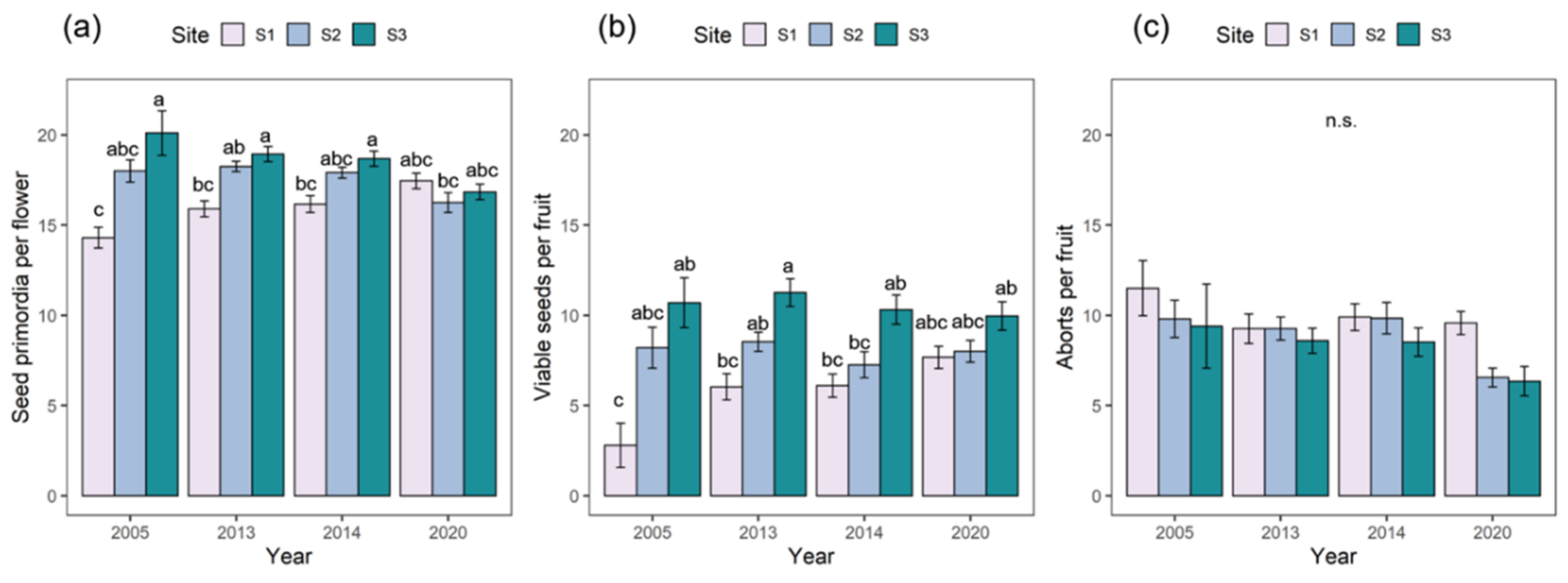
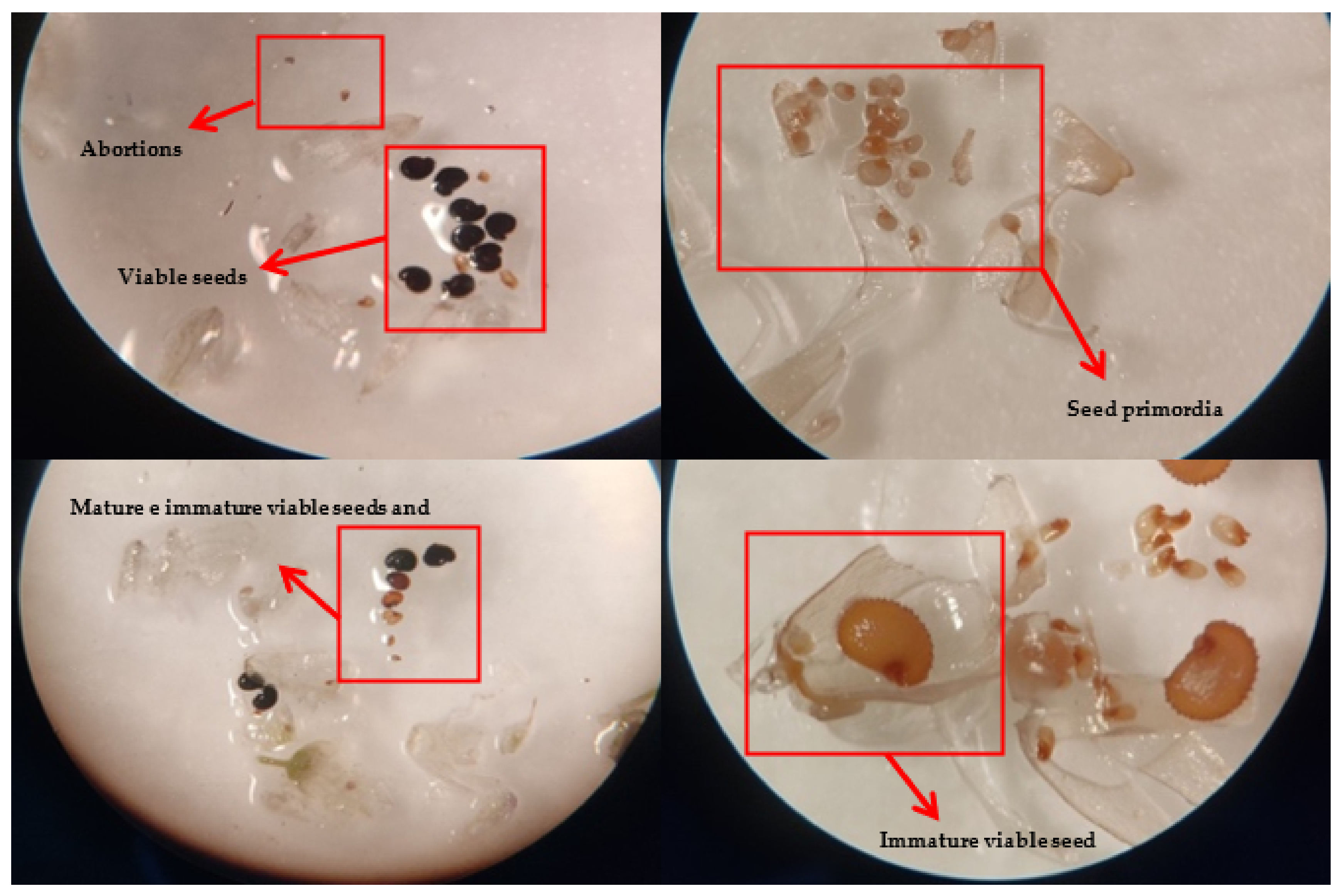
2.1. Reproductive Performance
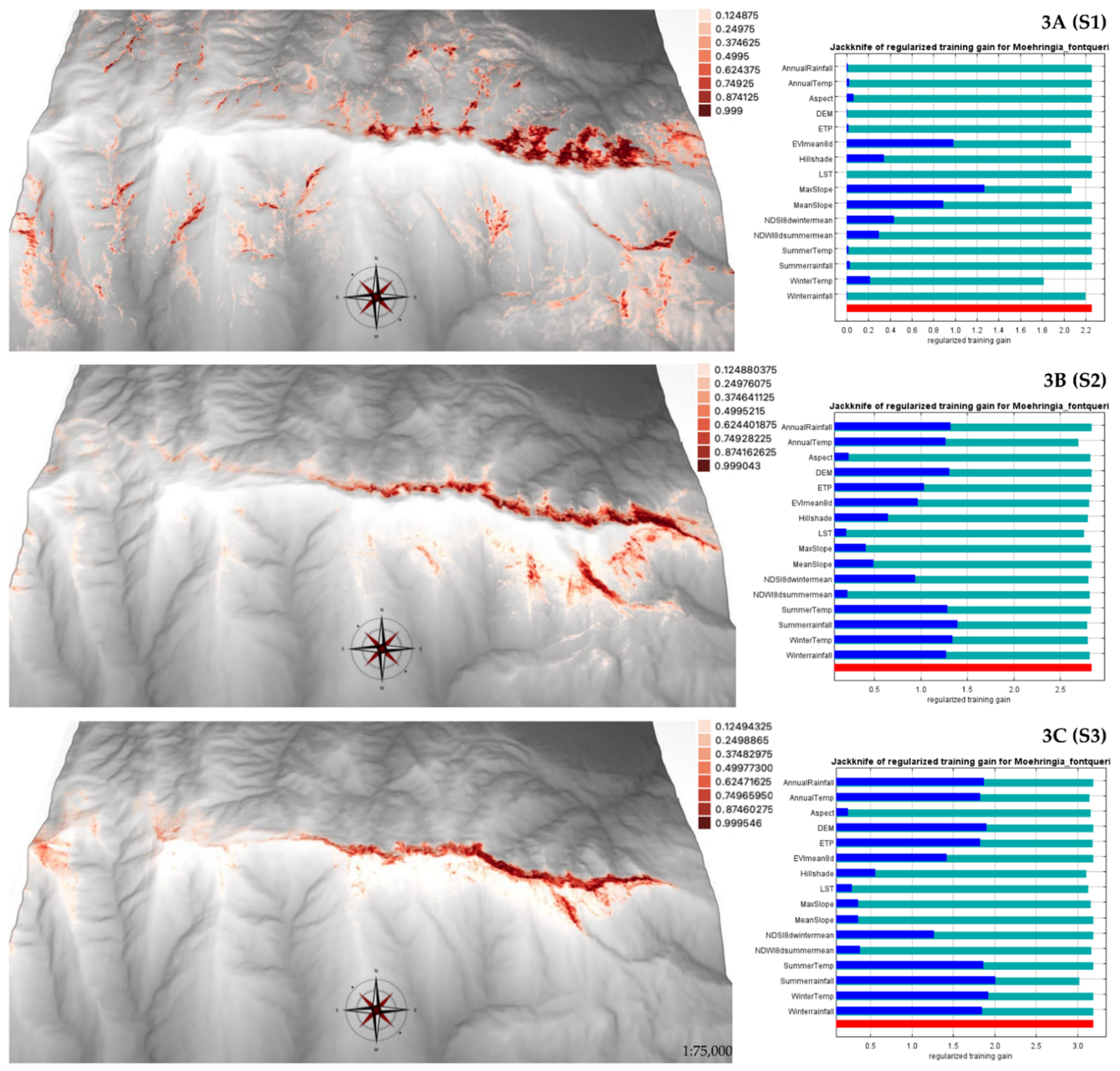
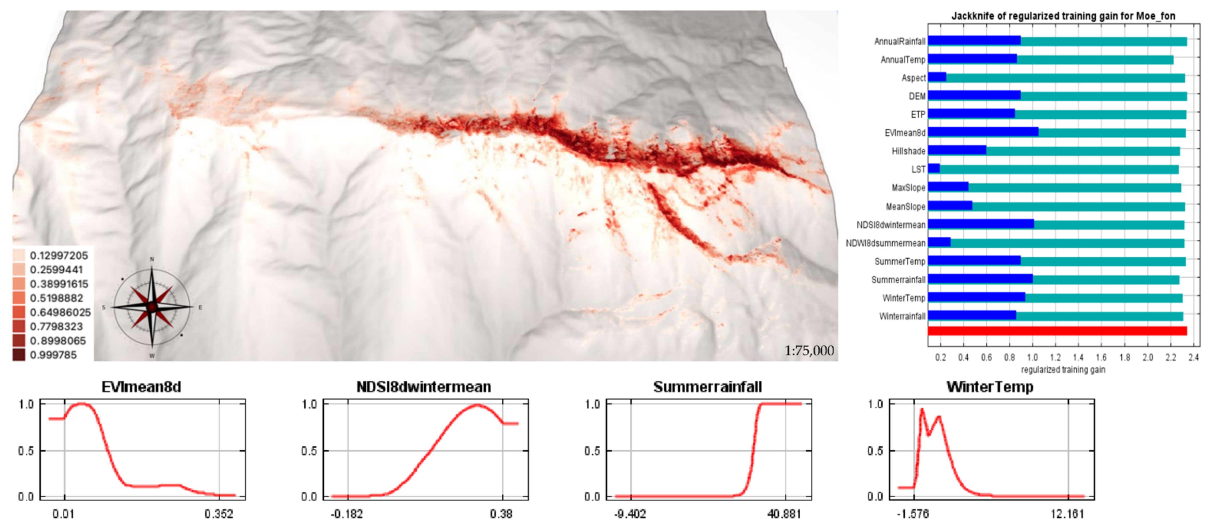
2.2. Current SDMs for M. fontqueri
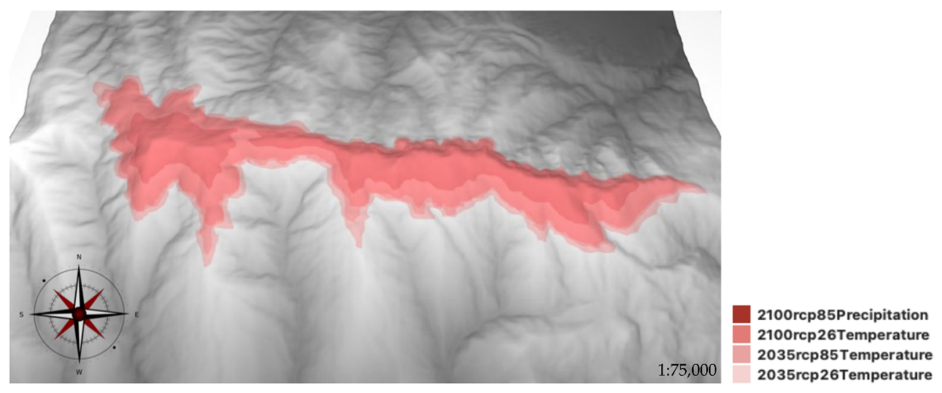
2.3. SDMs for M. fontqueri in Future Scenarios
3. Discussion
3.1. Reproductive Fitness of M. fontqueri
3.2. Current and Future Habitat Suitability
4. Materials and Methods
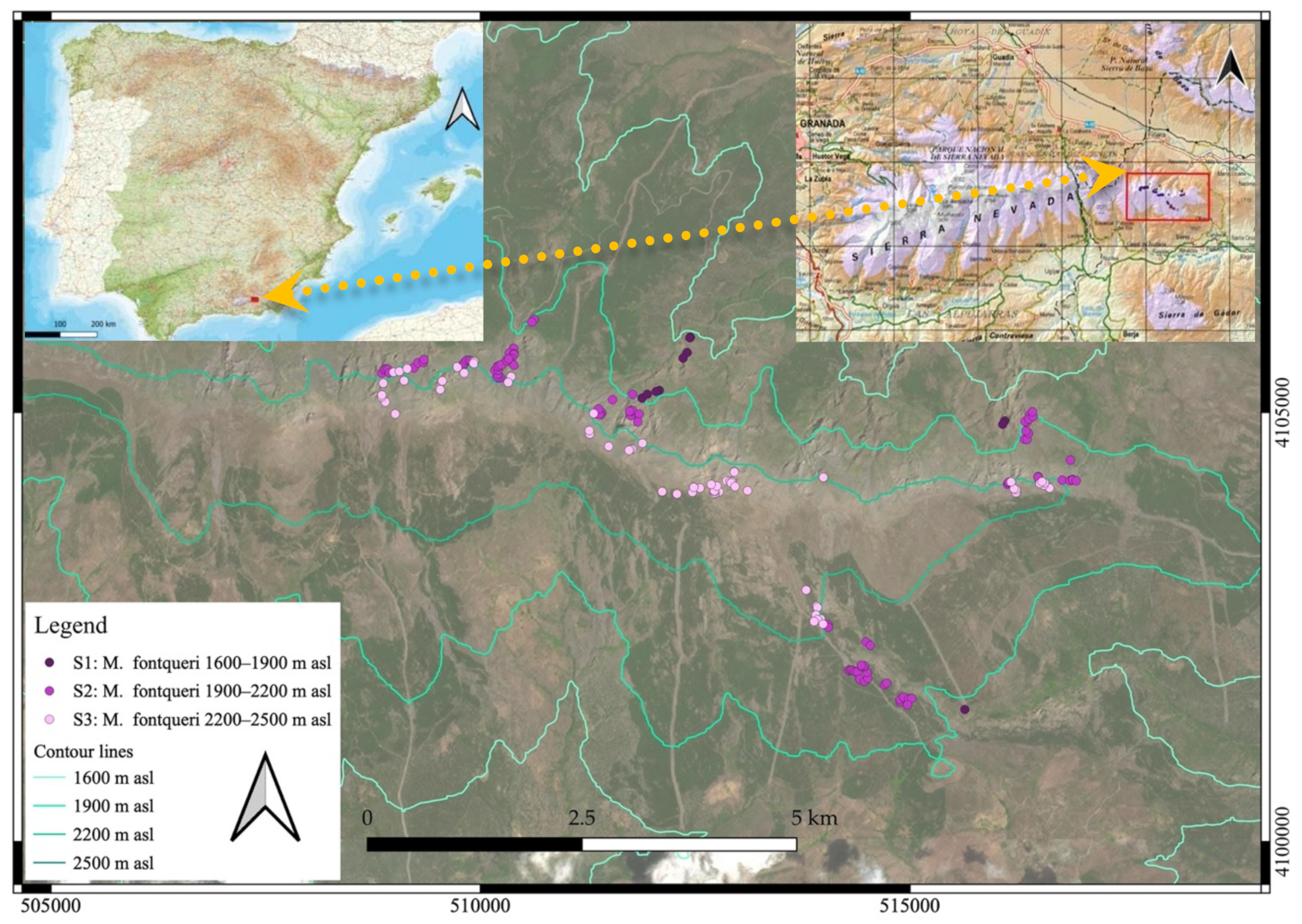
4.1. Study Area
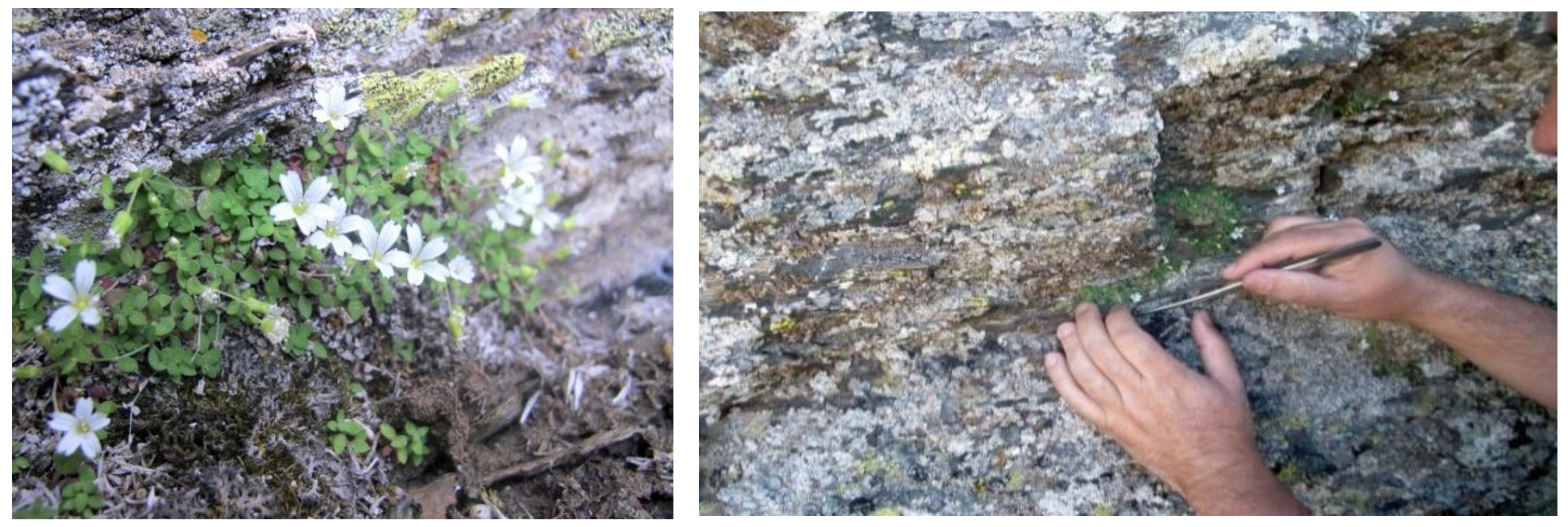
4.2. Study Species
4.3. Reproductive Biology
4.4. Data Analyses
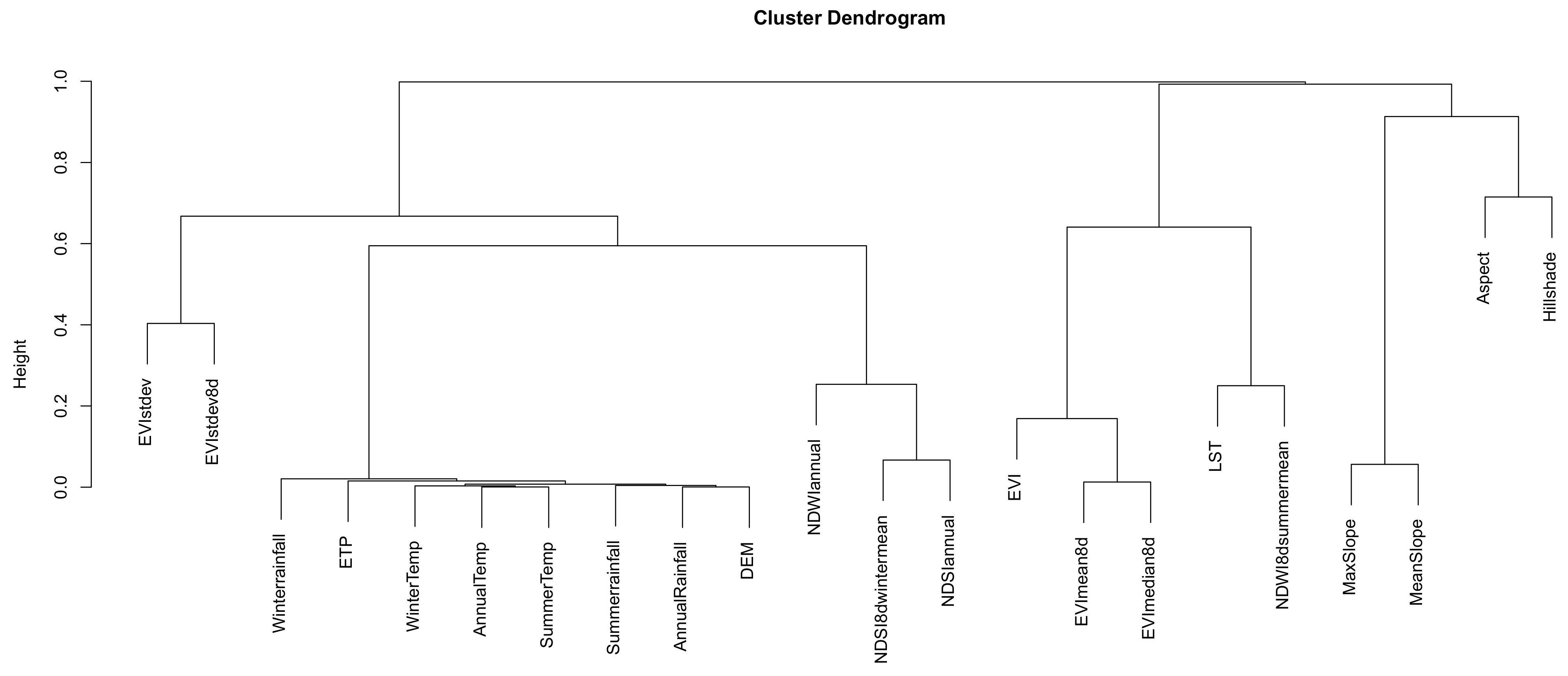
4.5. Current and Future Predictor Variables
4.6. SDMs and Ecological Niche
5. Conclusions
Author Contributions
Funding
Data Availability Statement
Acknowledgments
Conflicts of Interest
Appendix A

References
- Inouye, D.W. Effects of climate change on alpine plants and their pollinators. Ann. N. Y. Acad. Sci. 2020, 1469, 26–37. [Google Scholar] [CrossRef]
- Körner, C.; Paulsen, J. A world-wide study of high altitude treeline temperatures. J. Biogeogr. 2004, 31, 713–732. [Google Scholar] [CrossRef]
- Körner, C.; Paulsen, J.; Spehn, E.M. A definition of mountains and their bioclimatic belts for global comparisons of biodiversity data. Alp. Bot. 2011, 121, 73–78. [Google Scholar] [CrossRef] [Green Version]
- Myers, N.; Mittermeier, R.A.; Mittermeier, C.G.; da Fonseca, G.A.B.; Kent, J. Biodiversity hotspots for conservation priorities. Nature 2000, 403, 853–858. [Google Scholar] [CrossRef]
- Chape, S.; Spalding, M.; Jenkins, M.D. The World’s Protected Areas; Prepared by the UNEP World Conservation Monitoring Centre; University of California Press: Berkeley, CA, USA, 2008. [Google Scholar]
- Körner, C.; Jetz, W.; Paulsen, J.; Payne, D.; Rudmann-Maurer, K.; Spehn, E.M. A global inventory of mountains for bio-geographical applications. Alp. Bot. 2017, 127, 1–15. [Google Scholar] [CrossRef] [Green Version]
- Steinbauer, M.J.; Grytnes, J.A.; Jurasinski, G.; Kulonen, A.; Lenoir, J.; Pauli, H.; Rixen, C.; Winkler, M.; Bardy-Durchhalter, M.; Barni, E.; et al. Accelerated increase in plant species richness on mountain summits is linked to warming. Nature 2018, 556, 231–234. [Google Scholar] [CrossRef] [Green Version]
- Hughes, L. Biological consequences of global warming: Is the signal already apparent? Trends Ecol. Evol. 2000, 15, 56–61. [Google Scholar] [CrossRef]
- Körner, C. The use of ‘altitude’ in ecological research. Trends. Ecol. Evol. 2007, 22, 569–574. [Google Scholar] [CrossRef] [PubMed]
- Frei, E.; Bodin, J.; Walther, G.R. Plant species’ range shifts in mountainous areas-all uphill from here? Bot. Helv. 2010, 120, 117–128. [Google Scholar] [CrossRef] [Green Version]
- Lenoir, J.; Gégout, J.C.; Guisan, A.; Vittoz, P.; Wohlgemuth, T.; Zimmermann, N.E.; Dullinger, S.; Pauli, H.; Willner, W.; Svenning, J. Going against the flow: Potential mechanisms for unexpected downslope range shifts in a warming climate. Ecography 2010, 33, 295–303. [Google Scholar] [CrossRef]
- Walther, G.R.; Post, E.; Convey, P.; Menzel, A.; Parmesan, C.; Beebee, T.J.C.; Fromentin, J.; Hoegh-Guldberg, O.; Bairlein, F. Ecological responses to recent climate change. Nature 2002, 416, 389–395. [Google Scholar] [CrossRef] [PubMed]
- Grabherr, G.; Gottfried, M.; Pauli, H. Climate effects on mountain plants. Nature 1994, 369, 448. [Google Scholar] [CrossRef]
- Thuiller, W.; Lavorel, S.; Araújo, M.B.; Sykes, M.T.; Prentice, I.C. Climate change threats to plant diversity in Europe. Proc. Natl. Acad. Sci. USA 2005, 102, 8245–8250. [Google Scholar] [CrossRef] [PubMed] [Green Version]
- Nogués-Bravo, D.; Rodríguez, J.; Hortal, J.; Batra, P.; Araújo, M.B. Climate change, humans, and the extinction of the woolly mammoth. PLOS Biol. 2008, 6, e79. [Google Scholar] [CrossRef] [Green Version]
- Engler, R.; Randin, C.F.; Thuiller, W.; Dullinger, S.; Zimmermann, N.E.; Araújo, M.B.; Pearman, P.B.; Le Lay, G.; Piedallu, C.; Albert, C.H. 21st century climate change threatens mountain flora unequally across Europe. Glob. Change Biol. 2011, 17, 2330–2341. [Google Scholar] [CrossRef]
- Davis, M.B.; Shaw, R.G. Range shifts and adaptive responses to Quaternary climate change. Science 2001, 292, 673–679. [Google Scholar] [CrossRef] [Green Version]
- Thuiller, W.; Araújo, M.B.; Pearson, R.G.; Whittaker, R.J.; Brotons, L.; Lavorel, S. Biodiversity conservation: Uncertainty in predictions of extinction risk. Nature 2004, 430, 1–33. [Google Scholar] [CrossRef]
- Malhi, Y.; Franklin, J.; Seddon, N.; Solan, M.; Turner, M.G.; Field, C.B.; Knowlton, N. Climate change and ecosystems: Threats, opportunities and solutions. Phil. Trans. R. Soc. B 2020, 375, 2019010420190104. [Google Scholar] [CrossRef] [PubMed] [Green Version]
- Pauli, H.; Gottfried, M.; Dullinger, S.; Abdaladze, O.; Akhalkatsi, M.; Benito Alonso, J.L.; Coldea, G.; Dick, J.; Erschbamer, B.; Fernández Calzado, R.; et al. Recent Plant Diversity Changes on Europe’s Mountain Summits. Science 2012, 336, 353–355. [Google Scholar] [CrossRef] [Green Version]
- Gottfried, M.; Pauli, H.; Futschik, A.; Akhalkatsi, M.; Barančok, P.; Benito Alonso, J.L.; Coldea, G.; Dick, J.; Erschbamer, B.; Fernández Calzado, M.R.; et al. Continent-wide response of mountain vegetation to climate change. Nat. Clim. Change 2012, 2, 111–115. [Google Scholar] [CrossRef]
- Hamid, M.; Khuroo, A.A.; Malik, A.H.; Ahmad, R.; Singh, C.P.; Dolezal, J.; Haq, S.M. Early Evidence of Shifts in Alpine Summit Vegetation: A case study from Kashmir Himalaya. Front. Plant. Sci. 2020, 11, 421. [Google Scholar] [CrossRef] [Green Version]
- Benito, B.M.; Lorite, J.; Peñas, J. Simulating potential effects of climatic warming on altitudinal patterns of key species in Mediterranean-Alpine ecosystems. Clim. Change 2011, 108, 471–483. [Google Scholar] [CrossRef]
- Lamprecht, A.; Pauli, H.; Fernández-Calzado, M.R.; Lorite, J.; Molero Mesa, J.; Steinbauer, K.; Winkler, M. Changes in plant diversity in a water-limited and isolated high-mountain range (Sierra Nevada, Spain). Alp. Bot. 2021, 131, 27–39. [Google Scholar] [CrossRef]
- Forest, F.; Grenyer, R.; Rouget, M.; Davies, T.J.; Cowling, R.M.; Faith, D.P.; Balmford, A.; Manning, J.C.; Procheş, S.; van der Bank, M.; et al. Preserving the evolutionary potential of floras in biodiversity hotspots. Nature 2007, 445, 757–760. [Google Scholar] [CrossRef] [PubMed]
- Benito, B.M.; Lorite, J.; Pérez-Pérez, R.; Gómez-Aparicio, L.; Peñas, J. Forecasting plant range collapse in a mediterranean hotspot: When dispersal uncertainties matter. Divers. Distrib. 2014, 20, 72–83. [Google Scholar] [CrossRef] [Green Version]
- Lande, R. Risks of population extinction from demographic and environmental stochasticity and random catastrophes. Am. Nat. 1993, 142, 911. [Google Scholar] [CrossRef] [PubMed]
- Perrigo, A.; Hoorn, C.; Antonelli, A. Why mountains matter for biodiversity. J. Biogeogr. 2020, 47, 315–325. [Google Scholar] [CrossRef] [Green Version]
- Pérez-García, F.J.; Medina-Cazorla, J.M.; Martínez-Hernández, F.; Garrido-Becerra, J.A.; Mendoza-Fernández, A.J.; Salmerón-Sánchez, E.; Mota, J.F. Iberian Baetic endemic flora and the implications for a conservation policy. Ann. Bot. Fenn. 2012, 49, 43–54. [Google Scholar] [CrossRef]
- Holt, R.D. The microevolutionary consequences of climate change. Trends Ecol. Evol. 1990, 5, 311–315. [Google Scholar] [CrossRef]
- Salmerón-Sánchez, E.; Mendoza-Fernández, A.J.; Lorite, J.; Mota, J.F.; Peñas, J. Plant conservation in Mediterranean-type ecosystems. Mediterr. Bot. 2021, 42, e71333. [Google Scholar] [CrossRef]
- Guisan, A.; Zimmermann, N.E. Predictive habitat distribution models in ecology. Ecol. Model. 2000, 135, 147–186. [Google Scholar] [CrossRef]
- Lorite, J.; Gómez, F.; Mota, J.F.; Valle, F. Orophilous plant communities of Baetic range in Andalusia (south-eastern Spain): Priority altitudinal-islands for conservation. Phytocoenologia 2007, 37, 625. [Google Scholar] [CrossRef] [Green Version]
- Lembrechts, J.J.; Nijs, I.; Lenoir, J. Incorporating microclimate into species distribution models. Ecography 2019, 42, 1267–1279. [Google Scholar] [CrossRef]
- Guisan, A.; Thuiller, W. Predicting species distribution: Offering more than simple habitat models. Ecol. Lett. 2005, 8, 993–1009. [Google Scholar] [CrossRef] [PubMed]
- Araújo, M.B.; Guisan, A. Five (or so) challenges for species distribution modelling. J. Biogeogr. 2006, 33, 1677–1688. [Google Scholar] [CrossRef]
- IPCC. Global Warming of 1.5 °C (Summary for Policymakers); World Meteorological Organization: Geneva, Switzerland, 2008. [Google Scholar]
- Aguirre-Liguori, J.A.; Ramírez-Barahona, S.; Gaut, B.S. The evolutionary genomics of species’ responses to climate change. Nat. Ecol. Evol. 2021, 5, 1350–1360. [Google Scholar] [CrossRef] [PubMed]
- Araújo, M.B.; New, M. Ensemble forecasting of species distributions. Trends Ecol. Evol. 2007, 22, 42–47. [Google Scholar] [CrossRef]
- Nagy, L.; Grabherr, G. The Biology of Alpine Habitats; Oxford University Press: Oxford, UK, 2009. [Google Scholar]
- Lorite, J.; Lamprecht, A.; Peñas, J.; Rondinel-Mendoza, K.; Fernandez-Calzado, R.; Benito, B.; Cañadas, E. Altitudinal patterns and changes in the composition of high mountain plant communities. In The Landscape of the Sierra Nevada, 1st ed.; Zamora, R., Oliva, M., Eds.; Springer Nature Switzerland AG: Cham, Switzerland, 2022. [Google Scholar] [CrossRef]
- Peñas, J.; Pérez-García, F.; Mota, J.F. Patterns of endemic plants and biogeography of the Baetic high mountains (south Spain). Acta Bot. Gall. 2005, 152, 247–360. [Google Scholar] [CrossRef] [Green Version]
- Médail, F.; Diadema, K. Glacial refugia influence plant diversity patterns in the Mediterranean basin. J. Biogeogr. 2009, 36, 1333–1345. [Google Scholar] [CrossRef]
- Cañadas, E.M.; Giuseppe, F.; Peñas, J.; Lorite, J.; Mattana, E.; Bachetta, G. Hotspots within hotspots: Endemic plant richness, environmental drivers, and implications for conservation. Biol. Conserv. 2014, 170, 282–291. [Google Scholar] [CrossRef]
- Peñas, J.; Lorite, J. Biología de la Conservación de las Plantas de Sierra Nevada; Editorial Universidad de Granada: Granada, Spain, 2019. [Google Scholar]
- Bañares, Á.; Blanca, G.; Güemes, J.; Moreno, J.C.; Ortiz, S. Atlas de Flora Vascular Amenazada de España. Dirección General de Medio Natural y Política Forestal; Sociedad Española de Biología de la Conservación de Plantas: Madrid, Spain, 2011. [Google Scholar]
- Peñas, J.; Lorite, J. Moehringia fontqueri Pau. In Atlas y Libro Rojo de la Flora Vascular Amenazada de España, 1st ed.; Bañares, A., Blanca, G., Güemes, J., Moreno, J.C., Ortiz, S., Eds.; Dirección General de Medio Natural y Política Forestal, Sociedad Española de Biología de la Conservación de Plantas: Madrid, Spain, 2003; pp. 788–789. [Google Scholar]
- Lee-Yaw, J.A.; McCune, J.L.; Pironon, S.; Seema, N.S. Species distribution models rarely predict the biology of real populations. Ecography 2021, 2022, e05877. [Google Scholar] [CrossRef]
- Burgess, N.D.; Balmford, A.; Cordeiro, N.J.; Fjeldså, J.; Küper, W.; Rahbek, C.; Sanderson, E.W.; Scharlemann, J.P.W.; Sommer, J.H.; Williams, P.H. Correlations among species distributions, human density and human infrastructure across the high biodiversity tropical mountains of Africa. Biol. Conserv. 2007, 134, 164–177. [Google Scholar] [CrossRef]
- Giménez-Benavides, L.; Escudero, A.; García-Camacho, R.; García-Fernández, A.; Iriondo, J.M.; Lara-Romero, C.; Morente-López, J. How does climate change affect regeneration of Mediterranean high-mountain plants? An integration and synthesis of current knowledge. Plant Biol. 2018, 20, 50–62. [Google Scholar] [CrossRef] [PubMed]
- Scheepens, J.F.; Stöcklin, J. Flowering phenology and reproductive fitness along a mountain slope: Maladaptive responses to transplantation to a warmer climate in Campanula thyrsoides. Oecologia 2013, 171, 679–691. [Google Scholar] [CrossRef] [Green Version]
- Vitasse, Y.; Ursenbacher, S.; Klein, G.; Bohnenstengel, T.; Chittaro, Y.; Delestrade, A.; Monnerat, C.; Rebetez, M.; Rixen, C.; Strebel, N.; et al. Phenological and elevational shifts of plants, animals and fungi under climate change in the European Alps. Biol. Rev. 2021, 96, 1816–1835. [Google Scholar] [CrossRef] [PubMed]
- Gordo, O.; Sanz, J.J. Impact of climate change on plant phenology in Mediterranean ecosystems. Glob. Change Biol. 2010, 16, 1082–1106. [Google Scholar] [CrossRef]
- Gogol-Prokurat, M. Predicting habitat suitability for rare plants at local spatial scales using a species distribution model. Ecol. Appl. 2011, 21, 33–47. [Google Scholar] [CrossRef]
- DeMarche, M.L.; Doak, D.F.; Morris, W.F. Incorporating local adaptation into forecasts of species’ distribution and abundance under climate change. Glob. Change Biol. 2019, 25, 775–793. [Google Scholar] [CrossRef]
- Leandro, C.; Jay-Robert, P.; Mériguet, B.; Houard, X.; Renner, I.W. Is my sdm good enough? insights from a citizen science dataset in a point process modeling framework. Ecol. Model. 2020, 438, 109283. [Google Scholar] [CrossRef]
- Díaz de la Guardia, C.; Mota, J.F.; Valle, F. A new taxon in the genus Moehringia (Caryophyllaceae). Plant Syst. Evol. 1991, 177, 27–38. [Google Scholar] [CrossRef]
- Bradie, J.; Leung, B. A quantitative synthesis of the importance of variables used in MaxEnt species distribution models. J. Biogeogr. 2017, 44, 1344–1361. [Google Scholar] [CrossRef]
- Guillera-Arroita, G. Modelling of species distributions, range dynamics and communities under imperfect detection: Advances, challenges and opportunities. Ecography 2016, 40, 281–295. [Google Scholar] [CrossRef] [Green Version]
- Peñas, J.; Benito, B.; Lorite, J.; Ballesteros, M.; Cañadas, E.M.; Martínez-Ortega, M. Habitat fragmentation in arid zones: A case study of Linaria nigricans under land use changes (SE Spain). Environ. Manag. 2011, 48, 168–176. [Google Scholar] [CrossRef] [PubMed]
- Peñas, J.; Lorite, J. Moehringia fontqueri. The IUCN Red List of Threatened Species. Version 2015.1. 2013. Available online: www.iucnredlist.org (accessed on 16 September 2020).
- Qin, A.; Liu, B.; Guo, Q.; Bussmann, R.W.; Ma, F.; Jian, Z.; Xu, G.; Pei, S. Maxent modeling for predicting impacts of climate change on the potential distribution of Thuja sutchuenensis Franch, an extremely endangered conifer from southwestern China. Glob. Ecol. Conserv. 2017, 10, 139–146. [Google Scholar] [CrossRef]
- Fois, M.; Cuena-Lombraña, A.; Fenu, G.; Bacchetta, G. Using species distribution models at local scale to guide the search of poorly known species: Review, methodological issues and future directions. Ecol. Model. 2018, 385, 124–132. [Google Scholar] [CrossRef] [Green Version]
- Pepin, N.; Bradley, R.S.; Diaz, H.F.; Baraer, M.; Caceres, E.B.; Forsythe, N.; Fowler, H.; Greenwood, G.; Hashmi, M.Z.; Liu, X.D.; et al. Elevation-dependent warming in mountain regions of the world. Nat. Clim. Change 2015, 5, 424–430. [Google Scholar] [CrossRef] [Green Version]
- Blanca, G.; Cueto, M.; Martínez-Lirola, M.J.; Molero-Mesa, J. Threatened vascular flora of Sierra Nevada (southern Spain). Biol. Conserv. 1998, 85, 269–285. [Google Scholar] [CrossRef]
- Huelber, K.; Gottfried, M.; Pauli, H. Phenological Responses of Snowbed Species to Snow Removal Dates in the Central Alps: Implications for Climate Warming. Arct. Antarct. Alp. Res. 2006, 38, 99–103. [Google Scholar] [CrossRef]
- Post, E.S.; Pedersen, C.; Wilmers, C.C.; Forchhammer, M.C. Phenological sequences reveal aggregate life history response to climate warming. Ecology 2008, 89, 363–370. [Google Scholar] [CrossRef]
- Abdelaal, M.; Fois, M.; Fenu, G.; Bacchetta, G. Using MaxEnt modeling to predict the potential distribution of the endemic plant Rosa arabica Crép. in Egypt. Ecol. Inf. 2019, 50, 68–75. [Google Scholar] [CrossRef]
- Jiménez-García, D.; Peterson, A.T. Climate change impact on endangered cloud forest tree species in Mexico. Rev. Mex. Biodivers. 2019, 90, e902781. [Google Scholar] [CrossRef]
- Erfanian, M.B.; Sagharyan, M.; Memariani, F.; Ejtehadi, H. Predicting range shifts of three endangered endemic plants of the Khorassan-Kopet Dagh floristic province under global change. Sci. Rep. 2021, 11, 1–13. [Google Scholar] [CrossRef] [PubMed]
- Pitelka, L.F. Plant Migration Workshop Group. Plant Migration and Climate Change: A more realistic portrait of plant migration is essential to predicting biological responses to global warming in a world drastically altered by human activity. Am. Sci. 1997, 85, 464–473. [Google Scholar]
- Parmesan, C. Ecological and evolutionary responses to recent climate change. Annu. Rev. Ecol. Evol. 2006, 37, 637–669. [Google Scholar] [CrossRef] [Green Version]
- Dudley, L.S.; Arroyo, M.T.; Fernández-Murillo, M.P. Physiological and fitness response of flowers to temperature and water augmentation in a high Andean geophyte. Environ. Exp. Bot. 2018, 150, 1–8. [Google Scholar] [CrossRef]
- Hussain, S.; Lu, L.; Mubeen, M.; Nasim, W.; Karuppannan, S.; Fahad, S.; Tariq, A.; Mousa, B.G.; Mumtaz, F.; Aslam, M. Spatiotemporal variation in land use land cover in the response to local climate change using multispectral remote sensing data. Land 2022, 11, 595. [Google Scholar] [CrossRef]
- Shen, X.; Liu, B.; Jiang, M.; Lu, X. Marshland loss warms local land surface temperature in China. Geophys. Res. Lett. 2020, 47, e2020GL087648. [Google Scholar] [CrossRef] [Green Version]
- Shen, X.; Liu, Y.; Zhang, J.; Wang, Y.; Ma, R.; Liu, B.; Lu, X.; Jiang, M. Asymmetric impacts of diurnal warming on vegetation carbon sequestration of marshes in the Qinghai Tibet Plateau. Glob. Biogeochem. Cycles 2022, 36, e2022GB007396. [Google Scholar] [CrossRef]
- Pérez-Palazón, M.J.; Pimentel, R.; Herrero, J.; Aguilar, C.; Perales, J.M.; Polo, M.J. Extreme values of snow-related variables in Mediterranean regions: Trends and long-term forecasting in Sierra Nevada (Spain). Proc. IAHS 2015, 369, 157–162. [Google Scholar] [CrossRef] [Green Version]
- Burd, M. Bateman’s Principle and Plant Reproduction: The Role of Pollen Limitation in Fruit and Seed Set. Bot. Rev. 1994, 60, 83–139. [Google Scholar] [CrossRef]
- R Core Team. R: A Language and Environment for Statistical Computing; R Foundation for Statistical Computing: Vienna, Austria, 2020; Available online: https://www.R-project.org/ (accessed on 24 January 2020).
- de Mendiburu, F. Agricolae Statistical Procedures for Agricultural Research. R Package Version 1.3-1. 2019. Available online: https://CRAN.R-project.org/package=agricolae (accessed on 24 January 2020).
- Wickham, H. ggplot2: Elegant Graphics for Data Analysis; Springer: New York, NY, USA, 2016. [Google Scholar]
- Brooks, M.E.; Kristensen, K.; van Benthem, K.J.; Magnusson, A.; Berg, C.W.; Nielsen, A.; Skaug, H.J.; Mächler, M.; Bolker, B.M. glmmTMB Balances Speed and Flexibility Among Packages for Zero-inflated Generalized Linear Mixed Modeling. R J. 2017, 9, 378–400. [Google Scholar] [CrossRef] [Green Version]
- Hothorn, T.; Bretz, F.; Westfall, P.; Heiberger, R.M. multcomp: Simultaneous Inference in General Parametric Models. R Package Version 1.0-0. 2008. Available online: http://CRAN.R-project.org (accessed on 24 January 2020).
- Hartig, F. DHARMa: Residual Diagnostics for Hierarchical (Multi-Level/Mixed) Regression Models. 2021. Available online: https://cran.r-project.org/web/packages/DHARMa/vignettes/DHARMa.html (accessed on 24 January 2020).
- Farr, T.G.; Rosen, P.A.; Caro, E.; Crippen, R.; Duren, R.; Hensley, S.; Kobrick, M.; Paller, M.; Rodriguez, E.; Roth, L.; et al. The shuttle radar topography mission. Rev. Geophys. 2007, 2, RG2004. [Google Scholar] [CrossRef] [Green Version]
- NASA JPL. NASADEM Merged DEM Global 1 Arc Second V001 [Data Set]. In NASA EOSDIS Land Processes DAAC; 2020. Available online: https://data.nasa.gov/dataset/NASADEM-Merged-DEM-Global-1-arc-second-V001/dqg3-mwid/data (accessed on 11 November 2019).
- Huete, A.; Didan, K.; Miura, T.; Rodriguez, E.P.; Gao, X.; Ferreira, L.G. Overview of the radiometric and biophysical performance of the MODIS vegetation indices. Remote Sens. Environ. 2002, 83, 195–213. [Google Scholar] [CrossRef]
- Riggs, G.A.; Hall, D.K.; Salomonson, V.V. A snow index for the Landsat thematic mapper and moderate resolution imaging spectroradiometer. In Proceedings of the IGARSS’94-1994 IEEE International Geoscience and Remote Sensing Symposium, Pasadena, CA, USA, 8–12 August 1994. [Google Scholar] [CrossRef]
- Gao, B.C. NDWI-A normalized difference water index for remote sensing of vegetation liquid water from space. Remote Sens. Environ. 1996, 58, 257–266. [Google Scholar] [CrossRef]
- Jin, M.; Dickinson, R.E. Land surface skin temperature climatology: Benefitting from the strengths of satellite observations. Environ. Res. Lett. 2010, 5, 044004. [Google Scholar] [CrossRef] [Green Version]
- Austin, M.P.; Van Niel, K.P. Improving species distribution models for climate change studies: Variable selection and scale. J. Biogeogr. 2011, 38, 1–8. [Google Scholar] [CrossRef]
- Bruce, P.; Bruce, A. Practical Statistics for Data Scientists; O’Reilly Media, Inc.: Sebastopol, CA, USA, 2017. [Google Scholar]
- Fox, J. Applied Regression Analysis and Generalized Linear Models; Sage Publications: Thousand Oaks, CA, USA, 2016. [Google Scholar]
- Fox, J.; Monette, G. Generalized collinearity diagnostics. J. Am. Stat. Assoc. 1992, 87, 178–183. [Google Scholar] [CrossRef]
- Fox, J.; Weisberg, S. An R Companion to Applied Regression; Sage Publications: Thousand Oaks, CA, USA, 2011. [Google Scholar]
- Heiberger, R.M. HH: Statistical Analysis and Data Display: Heiberger and Holland; R Package: Vienna, Austria, 2020. [Google Scholar]
- Hijmans, R.J. raster: Geographic Data Analysis and Modeling; R Package Version 216, 2.8-4; R Package: Vienna, Austria, 2018. [Google Scholar]
- James, G.; Witten, D.; Hastie, T.; Tibshirani, R. An Introduction to Statistical Learning: With Applications in R; Springer Publishing Company: Berlin/Heidelberg, Germany, 2014. [Google Scholar]
- Dormann, C.F.; Elith, J.; Bacher, S.; Buchmann, C.; Carl, G.; Carré, G.; García Marquéz, J.R.; Gruber, B.; Lafourcade, B.; Leitão, P.J.; et al. Collinearity: A review of methods to deal with it and a simulation study evaluating their performance. Ecography 2013, 36, 27–46. [Google Scholar] [CrossRef]
- Phillips, S.J.; Anderson, R.P.; Schapire, R.E. Maximum entropy modeling of species geographic distributions. Ecol. Model. 2006, 190, 231–259. [Google Scholar] [CrossRef]
- Austin, M.P. Spatial prediction of species distribution: An interface between ecological theory and statistical modelling. Ecol. Model. 2002, 157, 101–118. [Google Scholar] [CrossRef] [Green Version]
- Elith, J.; Phillips, S.J.; Hastie, T.; Dudík, M.; Chee, Y.E.; Yates, C.J. A statistical explanation of MaxEnt for ecologists. Divers. Distrib. 2011, 17, 43–57. [Google Scholar] [CrossRef]
- Elith, J.; Graham, H.; Anderson, C.P.; Dudík, M.; Ferrier, S.; Guisan, A.; Hijmans, R.J.; Huettmann, F.; Leathwick, J.R.; Lehmann, A.; et al. Novel methods improve prediction of species’ distributions from occurrence data. Ecography 2006, 29, 129–151. [Google Scholar] [CrossRef] [Green Version]
- Morales, N.S.; Fernández, I.C.; Baca-González, V. MaxEnt’s parameter configuration and small samples: Are we paying attention to recommendations? A systematic review. PeerJ 2017, 5, e3093. [Google Scholar] [CrossRef] [PubMed]
- Pearson, R.G.; Raxworthy, C.J.; Nakamura, M.; Peterson, A.T. Predicting species distributions from small numbers of occurrence records: A test case using cryptic geckos in Madagascar. J. Biogeogr. 2007, 34, 102–117. [Google Scholar] [CrossRef]
- Swets, J.A. Measuring the accuracy of diagnostic systems. Science 1988, 240, 1285–1293. [Google Scholar] [CrossRef] [Green Version]
- Ashcroft, M.B.; French, K.O.; Chisholm, L.A. An evaluation of environmental factors affecting species distributions. Ecol. Model. 2001, 222, 524–531. [Google Scholar] [CrossRef] [Green Version]
- QGIS Development Team. QGIS Geographic Information System. 2020. Open Source Geospatial Foundation Project. Available online: https://www.qgis.org/es/site/ (accessed on 15 May 2022).
- Araújo, M.B.; Anderson, R.P.; Barbosa, A.M.; Beale, C.M.; Dormann, C.F.; Early, R.; Garcia, R.A.; Guisan, A.; Maiorano, L.; Naimi, B.; et al. Standards for distribution models in biodiversity assessments. Sci. Adv. 2019, 5, eaat4858. [Google Scholar] [CrossRef] [Green Version]
- Jump, A.S.; Woodward, F.I. Seed production and population density decline approaching the range-edge of Cirsium species. New Phytol. 2003, 160, 349–358. [Google Scholar] [CrossRef] [PubMed] [Green Version]
- Guo, Q.F.; Taper, M.; Schoenberger, M.; Brandle, J. Spatial-temporal population dynamics across species range: From centre to margin. Oikos 2005, 108, 47–57. [Google Scholar] [CrossRef]
- Hannah, L.; Midgley, G.F.; Lovejoy, T.E.; Bond, W.J.; Bush, M.; Lovett, J.C.; Scott, D.; Woodward, F.I. Conservation of Biodiversity in a Changing Climate. Conserv. Biol. 2002, 16, 264–268. [Google Scholar] [CrossRef]


| Seed Primordia per Flower | Viable Seeds per Flower | Aborted Seeds per Fruit | |||||
|---|---|---|---|---|---|---|---|
| df | χ2 | p | χ2 | p | χ2 | p | |
| Site | 2 | 23.11 | <0.001 | 63.69 | <0.001 | 9.73 | 0.01 |
| Year | 1 | 4.05 | 0.04 | 2.69 | 0.10 | 11.31 | <0.001 |
| Site × Year | 2 | 38.74 | <0.001 | 11.06 | <0.001 | 1.91 | 0.39 |
| Hypothesis | 95% Confidence Intervals for Group Differences | p-Value |
|---|---|---|
| S1 2005–S2 2013 | −7.2610–−0.6388 | 0.0036 |
| S1 2005–S3 2013 | −7.9930–−1.2820 | <0.001 |
| S1 2005–S2 2014 | −6.9620–−0.2504 | 0.0156 |
| S1 2005–S3 2014 | −7.7090–−1.0440 | <0.001 |
| S1 2005–S1 2020 | −6.3550–0.0526 | 0.0428 |
| S1 2005–S3 2005 | 1.6570–9.9430 | <0.001 |
| S3 2005–S1 2013 | 0.8281–7.5650 | 0.0017 |
| S3 2005–S1 2014 | 0.5510–7.3160 | 0.0053 |
| S1 2013–S2 2013 | −4.6160–−0.0771 | 0.0248 |
| S1 2013–S3 2013 | −5.3690–−0.6999 | <0.001 |
| S1 2013–S3 2014 | −5.0740–−0.4729 | 0.0030 |
| S2 2013–S2 2020 | −0.0423–4.0420 | 0.0447 |
| S3 2013–S1 2014 | 0.4168–5.1250 | 0.0044 |
| S3 2013–S2 2020 | 0.5735–4.8010 | 0.0012 |
| S3 2013–S3 2020 | −0.0489–4.2350 | 0.0457 |
| S1 2014–S3 2014 | −4.8300–−0.1895 | 0.0143 |
| S3 2014–S2 2020 | 0.3501–4.5030 | 0.0049 |
| Hypothesis | 95% Confidence Intervals for Group Differences | p-Value |
|---|---|---|
| S1 2005–S3 2005 | 2.1290–13.6700 | <0.001 |
| S3 2005–S1 2013 | −0.0250–9.3610 | 0.0379 |
| S3 2005–S1 2014 | −0.1120–9.3120 | 0.0459 |
| S1 2005–S1 2020 | −9.4800–−0.2536 | 0.0196 |
| S1 2005–S2 2013 | −10.4500–−1.0210 | 0.0026 |
| S1 2005–S2 2020 | −9.9770–−0.4227 | 0.0133 |
| S1 2005–S3 2013 | −13.2400–−3.6820 | <0.001 |
| S1 2005–S3 2014 | −12.2400–−2.7780 | <0.001 |
| S1 2005–S3 2020 | −11.9600–−2.3590 | <0.001 |
| S1 2013–S3 2013 | −8.6240–−1.8300 | <0.001 |
| S1 2013–S3 2014 | −7.6120–−0.9441 | 0.0010 |
| S1 2013–S3 2020 | −7.3610–−0.4974 | 0.0066 |
| S1 2014–S3 2013 | −8.5830–−1.7360 | <0.001 |
| S1 2014–S3 2014 | −7.5710–−0.8496 | 0.0016 |
| S1 2014–S3 2020 | −7.3190–−0.4036 | 0.0094 |
| S1 2020–S3 2013 | −6.8780–−0.3071 | 0.0125 |
| S2 2014–S3 2013 | −7.3980–−0.6040 | 0.0044 |
| Seed-Set | 2005 | 2013 | 2014 | 2020 |
|---|---|---|---|---|
| S1 | 20.84 | 37.38 | 36.73 | 44.00 |
| S2 | 45.32 | 49.55 | 41.92 | 49.23 |
| S3 | 57.10 | 59.45 | 55.20 | 59.14 |
| Elevational ranges | Area (km2) | Average Potential Habitat Suitability | SD | Variance |
|---|---|---|---|---|
| S1 (1600–1900 m asl) | 44.30 | 0.30 | 0.24 | 0.05 |
| S2 (1900–2200 m asl) | 36.58 | 0.16 | 0.18 | 0.03 |
| S3 (2200–2500 m asl) | 34.41 | 0.16 | 0.17 | 0.03 |
| Total study area | 79.98 | 0.15 | 0.18 | 0.03 |
| Scenarios | Area (km2) | Occurrences in Maximum Suitability Areas | Minimum Altitude (m asl) | Average Suitability ± SD | AUC |
|---|---|---|---|---|---|
| Current | 96.75 | 177 | 1637 | 0.1330 ± 0.0200 | 0.975 |
| 2035 RCP 2.6 | 49.00 | 128 (−49) | 2051 | 0.0039 ± 0.0004 | 0.988 |
| 2035 RCP 8.5 | 41.6 | 110 (−67) | 2113 | 0.0035 ± 0.0004 | 0.987 |
| 2100 RCP 2.6 | 37.47 | 103 (−74) | 2113 | 0.0029 ± 0.0005 | 0.987 |
| 2100 RCP 8.5 | 18.09 | 35 (−142) | 2259 | 0.0140 ± 0.0123 | 0.991 |
| Number of Flowers | Number of Fruits | ||||||||
|---|---|---|---|---|---|---|---|---|---|
| Main Locations Name and Elevation (m asl) | Elevational Ranges | 2005 | 2013 | 2014 | 2020 | 2005 | 2013 | 2014 | 2020 |
| S1: Barranco de la Campana (1960) | S1: 1600–1900 | 10 | 31 | 30 | 52 | 10 | 36 | 32 | 36 |
| S2: Between La Polarda and El Buitre (2150) | S2: 1900–2200 | 10 | 36 | 32 | 48 | 10 | 30 | 31 | 27 |
| S3: Under El Buitre summit (2430) | S3: 2200–2500 | 10 | 32 | 34 | 45 | 10 | 27 | 29 | 26 |
| Scenario | Average Annual Temperature | Average Winter Temperature | Average Summer Temperature | Average Annual Precipitation | Average Winter Temperature |
|---|---|---|---|---|---|
| 2035 RCP2.6 | +0.98 | +0.80 | +1.32 | −1.40% | −1.50% |
| 2035 RCP8.5 | +1.16 | +0.86 | +1.48 | −1.20% | −1.80% |
| 2100 RCP2.6 | +1.18 | +0.82 | +1.58 | −3.00% | −2.80% |
| 2100 RCP8.5 | +4.88 | +3.96 | +6.18 | −18.40% | −14.40% |
Publisher’s Note: MDPI stays neutral with regard to jurisdictional claims in published maps and institutional affiliations. |
© 2022 by the authors. Licensee MDPI, Basel, Switzerland. This article is an open access article distributed under the terms and conditions of the Creative Commons Attribution (CC BY) license (https://creativecommons.org/licenses/by/4.0/).
Share and Cite
Mendoza-Fernández, A.J.; Fernández-Ceular, Á.; Alcaraz-Segura, D.; Ballesteros, M.; Peñas, J. The Fate of Endemic Species Specialized in Island Habitat under Climate Change in a Mediterranean High Mountain. Plants 2022, 11, 3193. https://doi.org/10.3390/plants11233193
Mendoza-Fernández AJ, Fernández-Ceular Á, Alcaraz-Segura D, Ballesteros M, Peñas J. The Fate of Endemic Species Specialized in Island Habitat under Climate Change in a Mediterranean High Mountain. Plants. 2022; 11(23):3193. https://doi.org/10.3390/plants11233193
Chicago/Turabian StyleMendoza-Fernández, Antonio J., Ángel Fernández-Ceular, Domingo Alcaraz-Segura, Miguel Ballesteros, and Julio Peñas. 2022. "The Fate of Endemic Species Specialized in Island Habitat under Climate Change in a Mediterranean High Mountain" Plants 11, no. 23: 3193. https://doi.org/10.3390/plants11233193