1. Introduction
Recent advances in radio and processing technology have fuelled increased interest and adoption of localisation systems for both indoor and outdoor applications. Outdoor localisation applications, such as animal or people tracking, typically rely on GPS technology thanks to its high availability and accuracy. However, GPS modules are energy-hungry, which causes quick depletion of battery energy at resource-limited tracking devices.
Several recent proposals have attempted to address the energy consumption issue by duty cycling the GPS module and supplementing it with cellular tower signals [
1], local radio message exchanges [
2], and accelerometers [
3]. While all of these methods yield reductions in energy consumption, they still require the addition of extra modules into the devices for processing the supplementary signals. This limits the lifetime benefits of embedded devices that are desired in many long-term monitoring applications. For instance, applications that require inertial modules with tilt compensation and heading [
4] have an active power consumption that is comparable to a duty cycled GPS node. There have been limited attempts to duty cycle the supplementary modules, other than duty cycling of radio modules [
5].
This paper proposes duty cycling strategies for motion modules, in order to reduce their power consumption while maintaining their utility in supplementing GPS position information. Our strategies target applications that can tolerate a degree of positioning uncertainty. We adopt a motion-module duty cycling approach inspired from radio low power listening (LPL) [
6], where the motion module needs to wake up and obtain samples frequently enough to detect motion events (conceptually similar to transmit preambles). The main departure from LPL approaches is that we lack control of the motion event duration, thus we propose the selection of motion module duty cycles to capture the majority of motion events for a given application.
As an extension of this duty cycling approach, we introduce group-based duty cycling. Intuitively, nodes that cluster together can cooperatively share the burden of regularly checking for motion events, thereby reducing the energy cost for individual nodes. Nodes use periodic short range radio exchanges to track proximity contacts in the recent history. This history enables nodes to identify the subset of their neighbours whose movement has closely aligned with the nodes’ own movement patterns. Each node can then reduce the duty cycle of its motion sensor by up to the cardinality of that subset, as the movement of one of the nodes in the subset is indicative of movement of the whole group. Nodes broadcast radio beacons to all their neighbours when they detect motion, thus triggering sampling of motion sensors at these neighbours.
Our group-based duty cycling approach has broad applicability for tracking movement of people [
7] or animals [
5]. For instance, a group of people that are known to have close social links tend to cluster together, and their movements tend to be highly correlated. An example is a group of people in a theme park [
7], where the people tend to move together to attend meetings to visit certain attractions. Group-based duty cycling also applies for tracking the movement of many animal species that cluster together in large groups, including terrestrial species such as cattle, aerial species such as flying foxes, and aquatic species such as sardines.
This paper uses an empirical cattle tracking GPS data trace to evaluate our duty cycling strategies in simulations. The results enable the comparison of the individual and group strategies with previous methods in terms of power consumption and localisation accuracy. We find that both of our proposed strategies yield significant energy improvements over previous proposals at a slight reduction in location accuracy. We further determine that individual duty cycling is more suited towards higher mobility situations due to its deterministic sampling times, while the more space and time diverse sampling schedule of group duty cycling performs better for applications where motion events occur more rarely.
In summary, the contributions of this paper are three-fold:
Proposal of a motion sensor duty cycling strategy, based on learned motion features, for complementing GPS and radio duty cycling;
Extension of the strategy for a collaborative group-based approach;
Performance evaluation of the two strategies against previous work and in high and low mobility scenarios.
The remainder of the paper is organised as follows.
Section 2 reviews related work.
Section 3 provides the basis of our duty cycling approach.
Section 4 and
Section 5 present the individual and group duty cycling strategies respectively.
Section 6 compares the performance of these strategies in situations of high and low mobility.
Section 7 discusses the results, while
Section 8 concludes the paper.
2. Related Work
Li and Wu [
8] propose the use of a closeness metric between two nodes, defined as a measure of the frequency of encounters between two mobile nodes. To dynamically define communities, they rely on a threshold for the closeness metric, such that any group of nodes that are connected through edges with closeness metrics higher than the threshold are considered as a community. While we share the concept of a closeness threshold, we explore the effect of time and location of the closeness within existing communities, in order to predict emerging communities into the future.
An early instance of animal tracking by networked embedded systems is the ZebraNet project [
9], which tracks individual position records for animals every of a few minutes. However, ZebraNet collars include a solar panel, making the energy management problem quite a tractable one. Positioning is done by GPS only, and the nodes propagate their information by flooding in order to facilitate data acquisition by the mobile sink. The Networked Cow project [
10] used PDAs with GPS and
ad hoc WiFi to route position information to a base station.The Electronic Shepherd project [
1] also uses GPS localization for tracking herds of sheep in the mountains. “Real-time” is obtained thanks to a GPRS modems in the collar, even though position is recorded and sent back to base only a few times per day in order to prolong battery life. Unlike our work, nodes are asymmetric: only a few animals in the herd wear collars including GPS and GPRS modules. All the others wear a small ear-tag including only a microcontroller and a radio-chip.
The work in [
11] considers energy efficient localization for base nodes on the path of the mobile nodes and the energy implications of each approach. While the speed models in [
11] are similar to this paper, their work is purely simulation-based and does not consider the benefits of contact logging or online adaptation according to energy and position changes. The work in [
12] addresses the trade-off between localization accuracy and energy efficiency. It considers static, dynamic, and dead reckoning mobility models and studies their effect on accuracy and energy through ns2 simulations. Our work addresses the same tradeoff but uses empirical GPS data to conduct analysis on three different speed models and a realistic energy model of the GPS-enabled nodes that includes the previously unreported stochastic lock time model. We also consider the effect of dynamically changing the required localization performance based on the mobile node’s distance from an exclusion zone. Further we explore contact logging as a complement to GPS for achieving a better balance between accuracy and efficiency. In a similar fashion, Pattern
et al. [
13] provide a tuning knob to obtain various energy-accuracy trade-offs by the careful choice of duty cycle and activation radius.
The works in [
14,
15] address this trade-off as well by considering improvements to the RIP method [
16] as the baseline localization method. A key difference between You’s work and ours is that we support a variable uncertainty bound. Another distinction is their use of mote-based RSSI localization schemes in indoor environments, which require a deployed network infrastructure, consume less power, and require a calibration phase. Finally, they do not consider contact logging for reducing localization uncertainty.
Recent work [
2,
5,
17] has also explored collaborative localization that enables nodes to detect neighboring signals for position refinement. Chan
et al. [
17] use a cluster-based approach, where nearby nodes can establish clusters through IEEE 802.15.4 radios as a neighbour detection sensor that enhances WiFi localization. Our approach is similar in its reliance on contact signals, but it differs in that the contact signal is sent and received by the same radio, as in [
5], eliminating the need for multi-radio nodes.
More recently, research has explored energy-aware localization for mobile phones equipped with GPS. For example Constandache
et al. [
18] propose an average error metric for GPS duty cycling. Using proximity mechanisms like WiFi or GSM yields a lower average error for the same energy budget as plain GPS duty cycling. One of their mobility models deduces the current location of the node from recent history when the user is driving on a straight road. Similarly, the work in [
19] stores historical information of locations where GPS does not work, and of average speed as a function of time and place. The work in [
7] propose collaborative GPS localisation for people with smart phones in a theme park environment, confirming the dependence of the energy efficiency and accuracy of this approach on the radio range and uncertainty bound [
5].
The use of accelerometers has also been proposed as a low power indicator of movement to supplement GPS duty cycling [
19,
20]. Guo
et al. [
21] have used accelerometers, high sample rate GPS, and magnetometers to develop a cattle movement and behaviour model on which this paper builds. Kjaergaard
et al. [
22] use both accelerometers and magnetometers for energy efficient tracking, and consider individual duty cycling strategies for these components. Our approach differs from these works in that it considers group based duty cycling strategies for accelerometers or other motion detection sensors.
Other work has aimed at human tracking with the aid of accelerometers. For instance, Accelerometer Augmented Mobile Phone Localization (AAMPL) [
3] uses accelerometer to infer human activity, such as sitting or standing, through a centralised method. Similarly, Wang
et al. [
23] propose a classification method based on accelerometers for separating walking, running, stable and vehicle motion for humans. Rate-Adaptive GPS-based positioning for smartphones (RAPS) [
19] triggers GPS samples through accelerometers, as in our work. However, they are not using accelerometer as a boolean motion trigger, rather to measure an activity ratio computed over a time window. Unlike our strategy, their approach does not duty cycle the accelerometer.
3. Overview
In this paper, we develop algorithms for continuous tracking of mobile nodes based on their mobility features. Each node is equipped with a radio module for communication and contact logging, a motion detection module (such as a vibration sensor or accelerometer), and a GPS module for location estimation. Our goal is to determine duty cycles for the individual modules, so that the energy consumption of the overall system is minimised, while keeping the localisation error under a given threshold.
Previous work has shown that GPS duty cycling according to the average speed of nodes can reduce power consumption, and that the use of radio contact logging provides for further savings [
5]. Once a node acquires its position estimate through GPS, all neighbouring nodes within its radio broadcast range can estimate their locations accordingly. Here, we extend this work by using a motion detection module to detect when the nodes are stationary and subsequently turning off the GPS module, as in [
19]. This configuration can yield considerable savings, particularly for applications in which nodes are stationary for long periods, such as cattle grazing in a field.
Motion detection modules, however, still consume appreciable amounts of energy if running continuously. For instance, we use a Honeywell HMC6433 inertial module with accelerometer, magnetometer, heading and tilt compensation [
4] that can continuously draw about 6 mA of current. Keeping the inertial module active would have an equivalent energy cost to duty cycling the GPS module with contact logging [
5]. Therefore, efficient duty cycling of the motion detection modules is important for prolonging the system lifetime. We show that modelling the mobility of nodes enables efficient duty-cycling of accelerometers without sacrificing accuracy of motion detection. Specifically, energy savings on the order of the size of the group of nodes that travel together can be achieved compared with algorithms that consider individual nodes only. In the remainder of this section, we first motivate group based duty cycling through two applications, before presenting an overview of our duty cycling models.
3.1. Motivating Applications
A key motivating application for group-based duty cycling is to understand the behaviour of migratory birds [
24]. In particular, flying foxes are major cause for disease spread in both Australia and in Southeast Asia. These animals are highly mobile, traveling tens of kilometres in a single night and covering distances in excess of 1,000 km with the migratory season. In Australia, flying foxes are responsible for the spread of the Hendra virus, which is lethal to horses and harmful to humans. The processes and dynamics that underpin disease propagation within a group of flying foxes are not well understood, which is the main driver to monitor their movements and understand their behavior. Fortunately, these animals congregate at roosting camps and groups of tens of thousands of individuals and may remain there for days or weeks before moving to a new location. Using group based duty cycling therefore has huge potential for developing long-term tracking solutions for these animals. A related application is monitoring of livestock that also tends to form into long-term stable herds. The benefits of collaborative localisation for cattle have been demonstrated in [
5] through reliance on radio proximity data to reduce GPS duty cycles. In that earlier work, nodes did not have any inertial sensors. The animal scientists that wish to study the cattle behaviour are interested in high-quality inertial data from the animals while they are moving.
Both of the above applications require the use of inertial modules with tilt compensation and heading computation, which have a much higher energy consumption than basic inertial modules. The need to use higher energy inertial modules motivates duty cycling of these modules. In order to avoid missing motion events, multiple nodes that are clustered together in a group can cooperate on detecting motion in the group and simultaneously save energy.
3.2. Basic Assumptions and Definitions
We consider a set of nodes N = {Ni}, where Ni denotes an individual node. Our goal is to track location Li of each node over a set of discrete timestamps with a maximum user-set uncertainty. In order to ground the discussion, we consider accelerometers as our motion trigger modules, bearing in mind that the model applies equally to other motion sensors, such as gyroscopes and magnetometers.
Each node is equipped with a radio that has a perfectly circular range of
R meters. The nodes are further equipped with an accelerometer for motion detection, and a GPS module that estimates the node’s location
Li with an average uncertainty
Ugps meters. An accelerometer takes
tA time to estimate the node’s current speed, and the GPS module requires
tL seconds to achieve lock and return a location estimate. Because accelerometer readings are noisy and cannot reliably estimate fine-grained speed values, we use the accelerometer in our model to distinguish between two states: a stationary state and a moving state. The accelerometer can determine whether movement occurs through an internal mechanism that compares the measured speed with a user set speed threshold
![Jsan 01 00183 i006]()
3.2.1. Energy Model
We model node energy consumption by recording the duty cycles of the major node components: GPS module, radio, MCU, and inertial.
We compute the GPS and inertial module energy consumption at any time
t ring the deployment as
![Jsan 01 00183 i007]()
where
DCx is module
x’s duty cycle, and
![Jsan 01 00183 i008]()
is the power consumption of that module in active mode. Both modules are completely powered off when not in use, so they draw no current. We track the radio energy consumption as the sum of the transmission, reception, and listening energy values respectively [
25] for a given radio duty cycle, which is set to 10% in the rest of the paper (note that we do not consider radio state transition times in this paper for simplicity).
The MCU power consumption is heavily dependent on the duty cycling strategies of all the other components, as the MCU must power on when any of the other modules are active. In general, the MCU duty cycle and energy consumed are expressed as:
where DCgps, DCradio, and DCA are the duty cycles of the GPS, radio, and accelerometer respectively. The overlap parameter denotes any overlap between the on-times between these 3 components.
3.2.2. Metrics
We evaluate performance of the tracking algorithms developed in this paper using three main metrics. Power measured in milliwatts is calculated as the mean power consumed by a node over the course of the experiments. We further break down the total consumed power according to the individual hardware components. Error rate is a σ measure of the localisation accuracy of our algorithms. It is calculated as the percentage of times when the localisation error was larger than the reported uncertainty. Finally, AAU (absolute acceptable uncertainty) is a user-set bound on the maximum localisation uncertainty of the tracking algorithm.
3.3. GPS Duty Cycling with Radio Ranging
We consider an outdoor cattle tracking application using smart collars that contain wireless sensor nodes, GPS, and inertial modules with accelerometer, magnetometer, and hardware tilt compensation and heading calculation. The wireless sensor node is a Fleck [
26] comprising Atmel-1281 MCU and Atmel RF212 radio. Four D-Cell batteries in series provide power to all the collar components via several switch-mode regulators. The weight of these batteries yields a collar weight that approaches the upper limit set by an animal ethics committee, so larger batteries are not an option.
The target node lifetime in this application is 3 months, which is the interval at which the animals are brought in for health checks, treatment and sorting. Previous work had shown a significant increase in node lifetime with GPS duty cycling coupled with radio ranging [
5]. As our current work on collaborative localisation with accelerometer duty cycling builds on that earlier work, we briefly revisit it for presentation clarity.
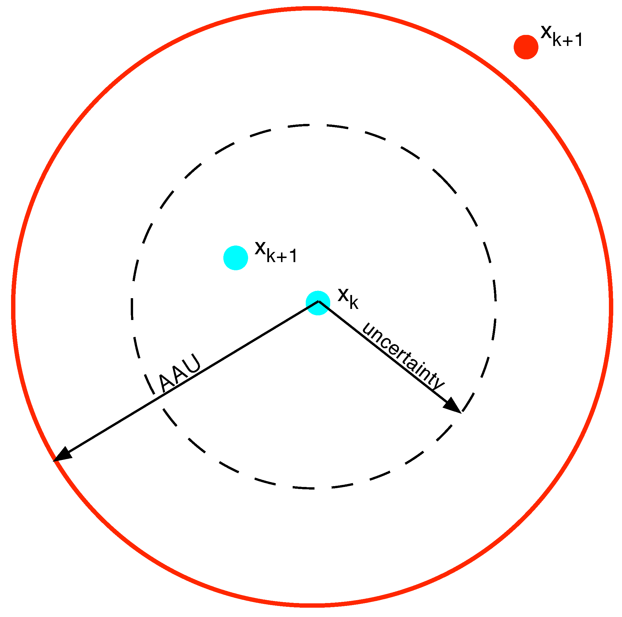
Figure 1 shows how GPS duty cycling works. At time
k we obtain a GPS measurement
xk and then turn off the GPS. At the next measurement
xk+1, the mobile node may be either within or outside the AAU, indicated by the larger circle. Whenever
xk+1 falls outside the larger circle, we denote this as an error, since the system would have failed to deliver a position estimate within the AAU.
This approach requires a means to estimate the uncertainty bound (shown as a dashed circle) at any given time. Since we do not know how fast or in what direction are the nodes moving, the simplest model is to assume a certain maximum speed and grow the estimated uncertainty linearly with time. When it approaches the AAU, taking into account the GPS’s lock time, we turn on the GPS. If the node’s speed exceeds our assumption, it could end up at the point marked in red when the GPS obtains a fix. This paper uses the dynamic speed model, which updates the assumed speed of a node every time it obtains a GPS lock [
5].
GPS lock can take several seconds, during which the module obtains an initial lock with a relatively high
Ugps, and then exponentially decreases its uncertainty as it receives more signals from visible satellites [
5]. Keeping the module on for longer yields higher position accuracy, but it incurs heavy energy cost. With the GPS duty cycling algorithm, a target GPS uncertainty can be set so that the total off time of the module (considering both the time spent obtaining lock and the time waiting for the algorithm uncertainty to grow) is minimised. Through offline calculations on the model in [
5], we determine this target GPS uncertainty to be 13 m for an AAU of 50 m. We use these settings for the rest of this paper for more aggressive GPS duty cycling.
Figure 1.
The growing uncertainty (dashed circle) and the maximum uncertainty bound (solid circle).
Figure 1.
The growing uncertainty (dashed circle) and the maximum uncertainty bound (solid circle).
Alongside GPS duty cycling, nodes use radio beacons to provide local position references. The beacons also include the sending node’s uncertainty. Whenever a node receives a beacon from a neighbour with a lower uncertainty, it adopts the position estimate of that neighbour and reduces its uncertainty according to its estimated distance from the neighbour. In order to receive radio messages, nodes use a low-power listening mechanism [
6]. Low power listening keep nodes’ radios in low-power sleep states for most of the time. The radio periodically wakes up for a short channel check assessment (CCA) time to check if there are any upcoming packet transmissions for this node. If so, the radio remains on to receive those packets. Otherwise, it goes back into sleep state. We use the same low-power listening approach for all radio beacons in this paper.
4. Individual Duty Cycling
In this section, we propose an algorithm for duty cycling of GPS and motion modules using data available locally on a sensor node. We first show that significant energy savings can be achieved if the motion sensing units are heavily duty cycled. We then model the behaviour of a tracked object stochastically as a Markov process. We assume that the object can be characterised by a set of discrete states and changes its state according to a set of fixed transition probabilities. The values of the probabilities heavily depend on contextual information. We assume they can be determined a priori or learned over the lifetime of the tracking system.
We use empirical data traces from 30 cow collar nodes collected continuously at 1 Hz over 2 days from a herd at the Belmont Research Station in central Queensland, in order to understand the performance of our algorithms on the basis of the behaviour of the tracked animals. We define a stationary and a motion state and study probabilities of transitioning between them. Given these probabilities, we find optimal values to sample motion sensors and update uncertainty of the location estimates.
4.1. Accelerometer Energy Consumption
While the earlier work focused on bounding the location uncertainty by growing it linearly over time according to an assumed speed [
5], accelerometers enable nodes to keep their uncertainty constant over long periods and thus reduce the duty cycle of the node’s MCU and GPS units. However, simply including an always-on accelerometer within the node is not energy-efficient, particularly for modules with heading and tilt compensation.
Table 1 shows the power consumption of the various node components in both active and sleep modes. Our earlier work had shown that GPS Duty cycling with radio proximity can achieve a combined power consumption for the GPS, radio, and MCU around 22 mW. In comparison, the inertial module would consume 18 mW if it remains in active mode all of the time, representing an 82% increase in overall power consumption for the node. While we expect the inclusion of the inertial module to reduce the duty cycles and energy consumption of the other node modules, any energy savings are likely to be outweighed by the increased energy consumption for powering the inertial module. Therein lies the need for aggressive duty cycling of the inertial module. The following sections explore the extent to which individual accelerometer duty cycling can improve the previous GPS/radio ranging strategy.
Table 1.
Active and sleep mode power consumption for node components.
Table 1.
Active and sleep mode power consumption for node components.
| Component | Active Mode Power (mW) | Sleep Mode Power (mW) |
|---|
| MCU | 18 | 1.2 |
| Radio (TX) | 79.2 | 0.00825 |
| Radio (RX) | 29.7 | 0.00825 |
| GPS | 165 | 0.215 |
| Accelerometer | 18 | 0 |
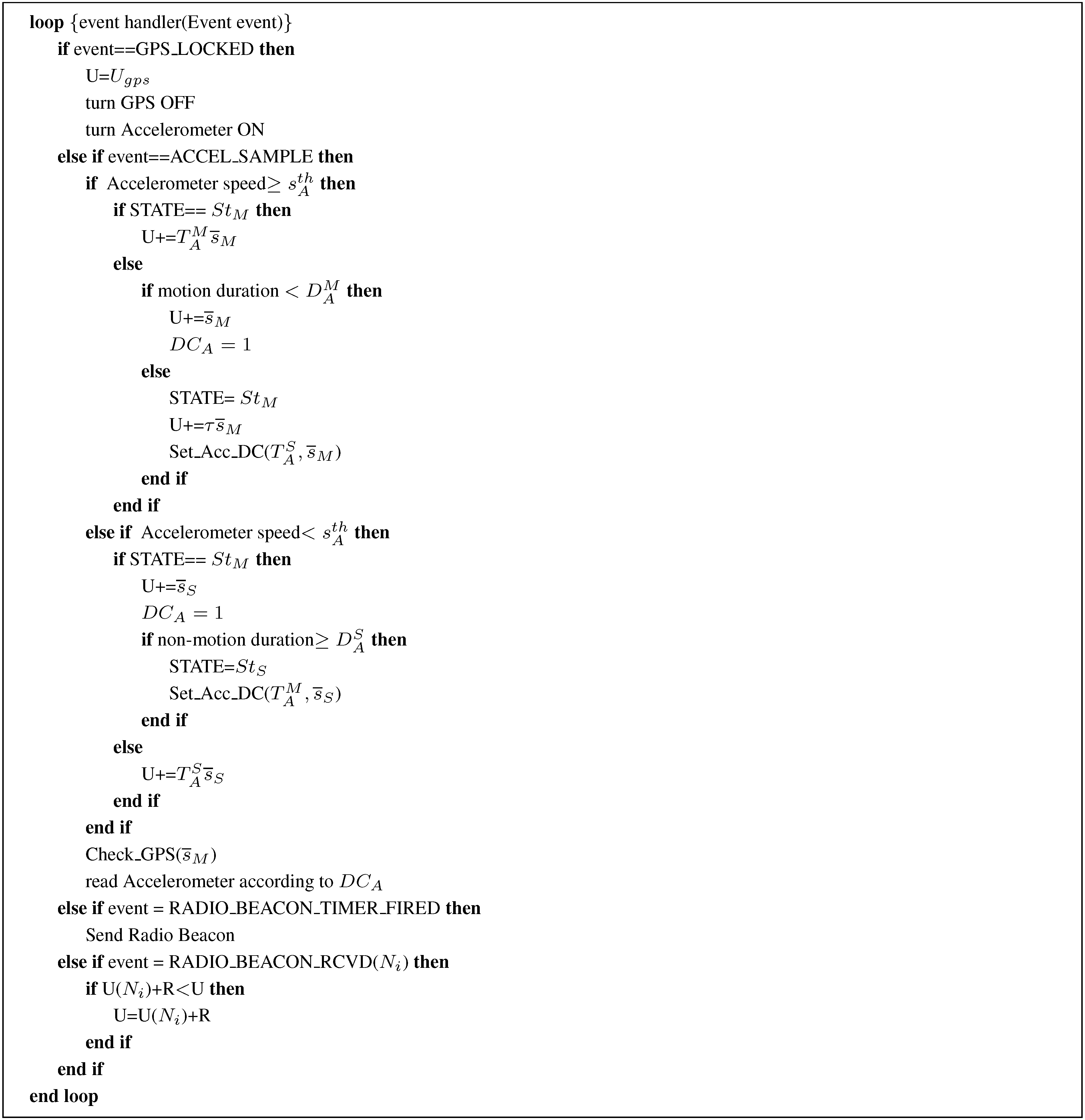
4.2. Duty Cycling Algorithm
This strategy enables nodes to set their accelerometer duty cycle independently of any neighbours. The individual duty cycling approach follows a state-based approach with two states: motion state
StM and stationary state
StS. The node uses the accelerometer to detect motion and defines
StM state for speeds above threshold
![Jsan 01 00183 i006]()
and
StS for speeds lower than the threshold. The individual duty cycling algorithm is shown in
Figure 2, while
Figure 3 shows a typical duty cycling scenario.
Figure 2.
Accelerometer Individual Duty Cycling Strategy.
Figure 2.
Accelerometer Individual Duty Cycling Strategy.
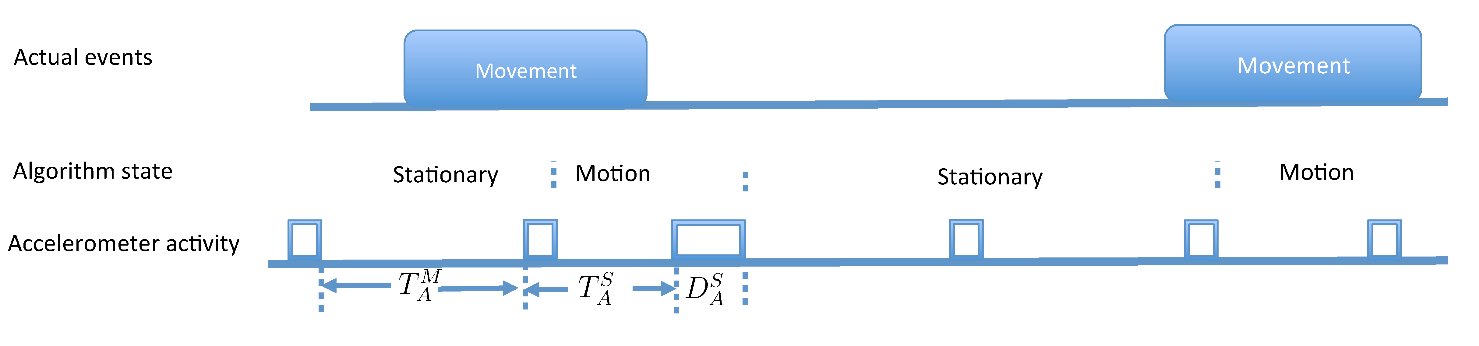
Figure 3.
Accelerometer Duty Cycling: showing a timeline of actual motion events, algorithm state, and the active/sleep periods of the accelerometer.
Figure 3.
Accelerometer Duty Cycling: showing a timeline of actual motion events, algorithm state, and the active/sleep periods of the accelerometer.
4.2.1. Travel and Resting Times
We duty cycle the accelerometer in both the motion and the stationary states. A key consideration in accelerometer duty cycling is the length of the off periods between subsequent accelerometer sampling periods. The lengths of the off periods for the accelerometer are based on two parameters: the minimum time
TM that a node is moving and the minimum time
TS that a node is stationary. Since a node is moving for at least
TM seconds, a duty cycled accelerometer will detect motion if it turns on once every
![Jsan 01 00183 i014]()
seconds in
StS, where
ε is a positive small number. Similarly, the accelerometer will detect a node being stationary if it turns on once every
![Jsan 01 00183 i009]()
seconds in the motion state
StM.
4.2.2. Uncertainty Estimation
Transitions between motion and stationary states are triggered by the node speed falling below or above the threshold
![Jsan 01 00183 i006]()
. To avoid spurious state transitions, we require the accelerometer to detect motion or non-motion for the duration of at least
![Jsan 01 00183 i010]()
and
![Jsan 01 00183 i011]()
seconds, respectively. The accelerometer detects motion or non-motion by checking the amplitude of its measured signal with a predefined threshold. Nodes increase their uncertainty in both states. In the stationary state, we increase uncertainty assuming that a node is moving at a slow
![Jsan 01 00183 i012]()
speed. This allows us to account for slow movement events such as cattle feeding, where a node moves slower than the threshold
![Jsan 01 00183 i006]()
for extended periods of time. On the other hand, in the motion state
StM, nodes update their uncertainty using their current speed estimate
![Jsan 01 00183 i013]()
. Finally, a node also updates its uncertainty when transitioning to the
StM state:
where
![Jsan 01 00183 i015]()
is the current speed estimate and
![Jsan 01 00183 i016]()
is proportional to the minimum travel time
![Jsan 01 00183 i017]()
.
λ is a constant between 0 and 1. For a conservative uncertainty estimate, the node sets
![Jsan 01 00183 i018]()
, assuming the worst case scenario that the node missed the first
![Jsan 01 00183 i017]()
seconds of the motion event. A less conservative approach is to increase its uncertainty by
![Jsan 01 00183 i019]()
, as the length of time that has already passed for the motion event is a uniformly distributed value between 0 and
![Jsan 01 00183 i017]()
.
4.2.3. Duty Cycle Setting
When the uncertainty grows close to AAU, a node powers on its GPS module. When the GPS locks in, the node powers off the GPS module and turns on the accelerometer for the motion detection. As
Figure 2 shows, the uncertainty U is also updated to the GPS module uncertainty when the GPS module gets a lock.
When the node is in the
StM state with its GPS off, it duty cycles its accelerometer with duty cycle
![Jsan 01 00183 i020]()
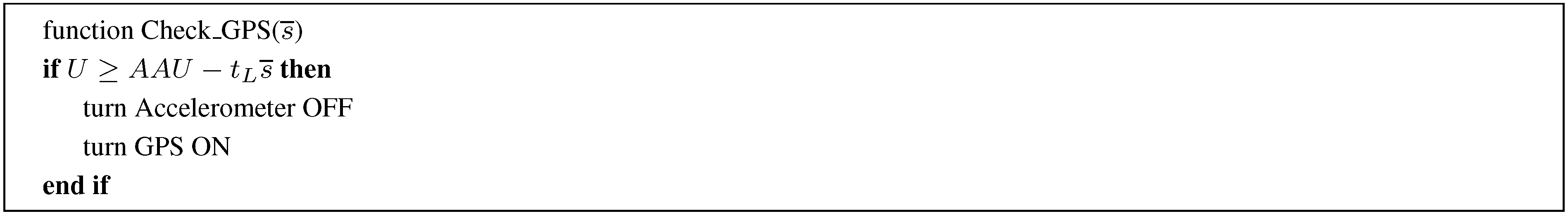
as long as motion continues and increases uncertainty accordingly. Every time instant that it increases its uncertainty, the node checks whether the uncertainty has reached a critical threshold by calling the Check_GPS() function (see
Figure 4). If so, the node activates its GPS module to start the GPS lock process and powers off its accelerometer.
Figure 4.
The Check_GPS() function.
Figure 4.
The Check_GPS() function.
If the node’s accelerometer detects that it has stopped moving, the node moves back to the
StS state, where it increases its uncertainty at a slower rate and reduces the accelerometer duty cycle to
![Jsan 01 00183 i021]()
. The function Set_Acc_DC() (see
Figure 5) determines the suitable off time for the accelerometer for both motion and stationary states. This will depend on the current value of the node’s uncertainty. Note that a node must power on its GPS module at least
tL seconds prior to its uncertainty reaching AAU, in order to account for the uncertainty growth during the GPS lock process. If a node’s uncertainty is much lower than this bound, then it can set its sleep time to
TA. However, if a node that is duty cycling its accelerometer detects motion when its uncertainty is slightly below or exactly AAU-
![Jsan 01 00183 i022]()
, then it must increase its uncertainty by
![Jsan 01 00183 i023]()
, resulting in an uncertainty of
![Jsan 01 00183 i024]()
. Even if the node powers on its GPS module at this instant, it is likely to have an uncertainty that exceeds AAU by the time it gets GPS lock. To avoid this situation, a node checks whether its uncertainty is greater than
![Jsan 01 00183 i025]()
. If so, the node anticipates that it may have to incorporate a step increase in its uncertainty when it detects motion, so it sets an instantaneous value of
TA to ensure that it will power on its GPS module at the right time:
The value of τ is then simply computed as λTA.
Figure 5.
The Set_Acc_DC() function.
Figure 5.
The Set_Acc_DC() function.
The individual duty cycling algorithm uses periodic radio beaconing, in order to quickly correct large uncertainty increases that result from short-term motion events (see
Figure 6 for an example). Periodic beaconing incurs a radio energy overhead over event-based beaconing [
5], but our results in this paper show that the energy savings with this algorithm outweigh the periodic beaconing overhead.
Figure 6.
The growth of uncertainty with accelerometer duty cycling. The narrow peaks correspond to accelerometer motion detection.
Figure 6.
The growth of uncertainty with accelerometer duty cycling. The narrow peaks correspond to accelerometer motion detection.
4.3. Example
We augment the python simulator in [
5] with the accelerometer duty cycling algorithm and energy model to evaluate their performance with our empirical cattle GPS data trace.
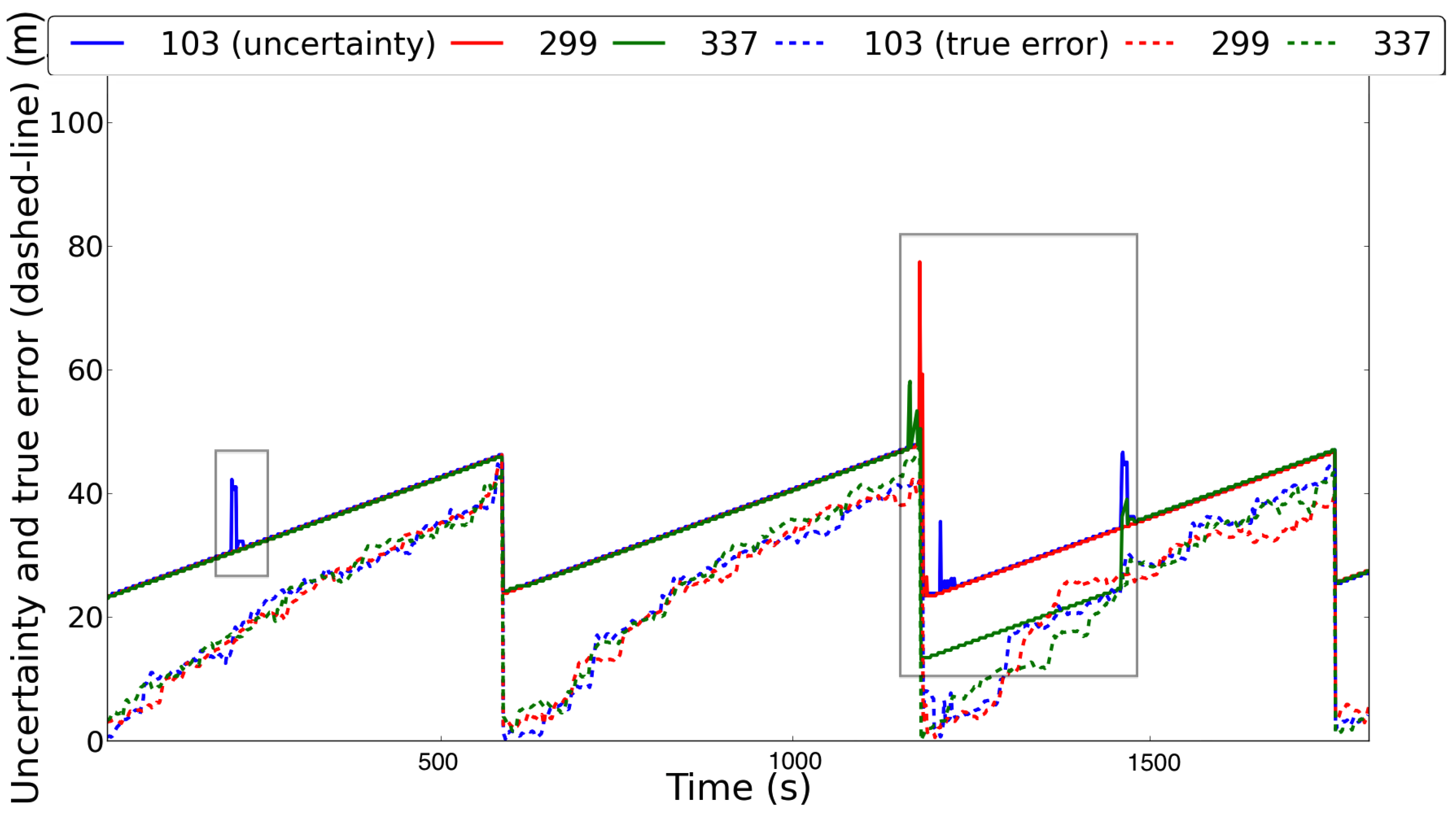
Figure 6 shows a trace of the uncertainty growth for 3 nodes from our empirical cattle dataset. The trace uses solid lines to indicate the algorithm uncertainty and dashed lines to indicate the true error for each node. At the start of the trace, all three nodes are growing their uncertainty linearly according to
![Jsan 01 00183 i012]()
, after having logged contact with a common neighbour 104, whose trace is not shown here. All of the narrow peaks in the trace indicate a node detecting motion after sampling its accelerometer, and adding a step increase to its uncertainty. The reason that the uncertainty drops back again is that the node mobility is transient and the nodes receive periodic contact beacons from neighbours that have a lower uncertainty shortly thereafter, which enables the nodes to lower their own uncertainty. It is specifically for this reason that the individual duty cycling algorithm has to use periodic radio beaconing (rather than event-based beaconing), in order to avoid premature GPS locks due to short-lived motion events.
Interesting situations arise at times 400 and 1,500. At 400 s, nodes 299 and 337 both detect motion independently, but in this case, they cannot lower their uncertainty after they leave the motion state because they do not receive any contact beacons with sufficiently low uncertainty. This situation persists until a neighbour acquires GPS lock, which enables all three nodes in the trace to lower their uncertainty by logging contact with that neighbour. At time 1,500, node 337 first detects brief motion, which causes a spike in its uncertainty. Once its accelerometer detects that it has stopped moving, it returns to a slow linear increase in uncertainty thanks to contact logs with node 299. A similar pattern occurs at node 103 about 100 s later. After that, node 299 detects that it is moving, and adds a step increase to its uncertainty. Note that the actual position error remains within the uncertainty at all times.
4.4. Parameter Settings and Tradeoffs
We focus on two performance parameters: energy consumption and localization error of the duty-cycled algorithm. Specifically, we would like to minimise the energy consumption of each node while keeping the localization error within a maximum uncertainty AAU and the error rate σ within an error tolerance σ* of 5%, because the animal scientists who are interested in the tracking data can accept a 95% success rate for the algorithm. If the duty cycle is low, we save more energy but increase the latency of motion detection, which can compromise the AAU uncertainty bound. All references to AAU error refer to the percentage of instances that the tracking algorithm exceeds the user-set maximum error.
4.4.1. Stationary State
We are interested in two main parameters in the stationary state. The minimum travel time allows us to set accelerometer duty cycle while making sure that we detect the majority of the motion events.
We use our cattle dataset, which contains GPS traces at 1 Hz for 35 nodes over two days, to determine its minimum travel duration. We define a speed threshold
![Jsan 01 00183 i006]()
of 0.4 m/s, above which nodes are considered to be in a motion state [
21].
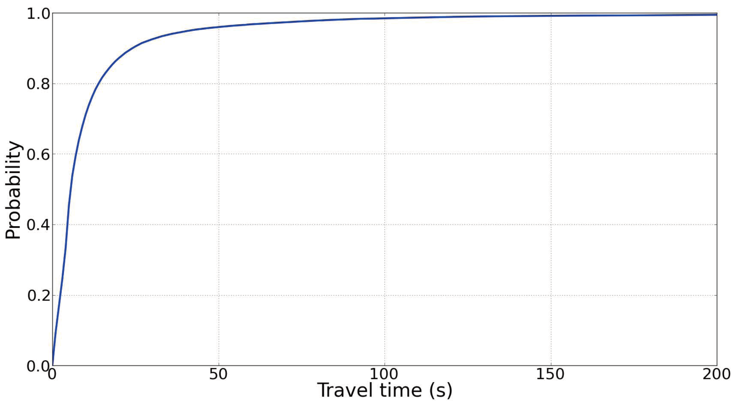
Figure 7 shows the cumulative distribution function of all movement states in the cattle trace, revealing that almost all movements persist for at least 5 s.
Figure 7.
The cumulative distribution function of movement durations for a speed threshold of 0.4 m/s. The minimum movement duration is around 5 s.
Figure 7.
The cumulative distribution function of movement durations for a speed threshold of 0.4 m/s. The minimum movement duration is around 5 s.
We run simulations of our duty cycling strategy on the cattle data trace with varying
TM.
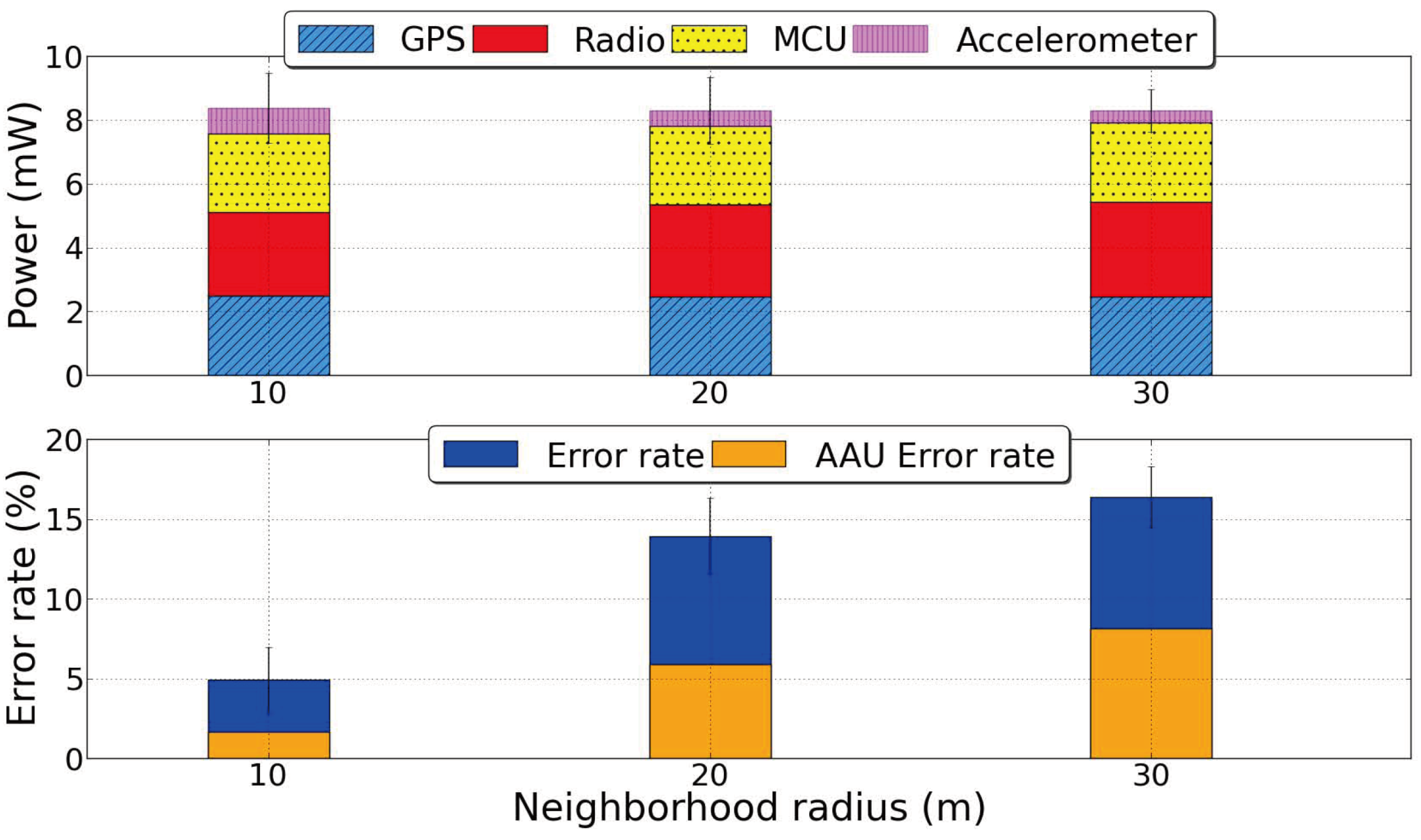
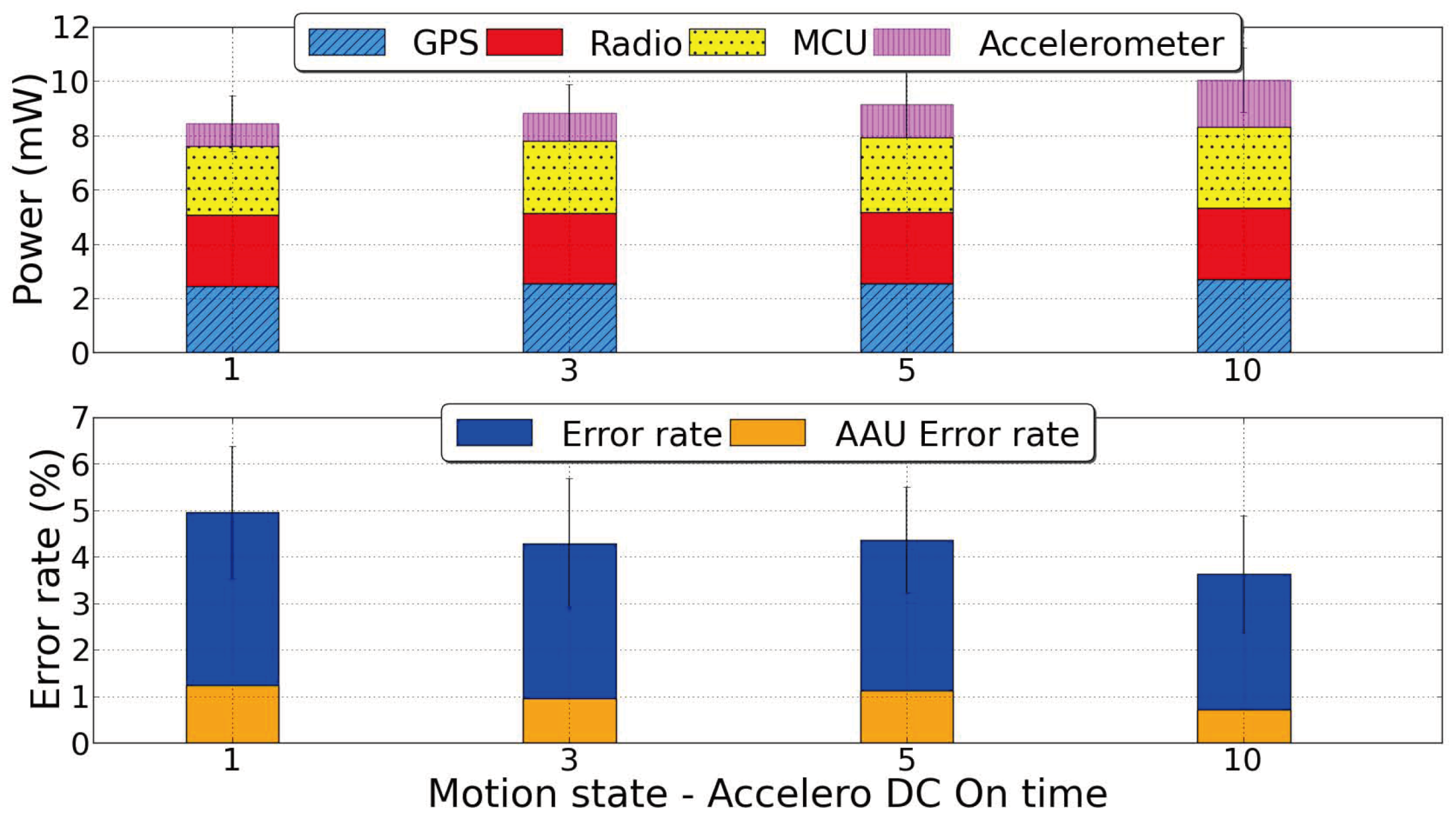
Figure 8 shows the energy consumption and error rates for the different
TM values. The minimum travel time setting can clearly deliver a range of positioning accuracies (between 92% and 99%) while trading off energy consumption. Because our target application has an error tolerance of 5%, we set a minimum travel time
TM of 30 s as the most energy-efficient choice, with a power consumption around 8 mW.
Figure 8.
The impact of varying TM on node energy consumption and error rates. The AAU error rate refers to the errors observed in the online algorithm, while the error rate refers to all the errors based on ground truth positions.
Figure 8.
The impact of varying TM on node energy consumption and error rates. The AAU error rate refers to the errors observed in the online algorithm, while the error rate refers to all the errors based on ground truth positions.
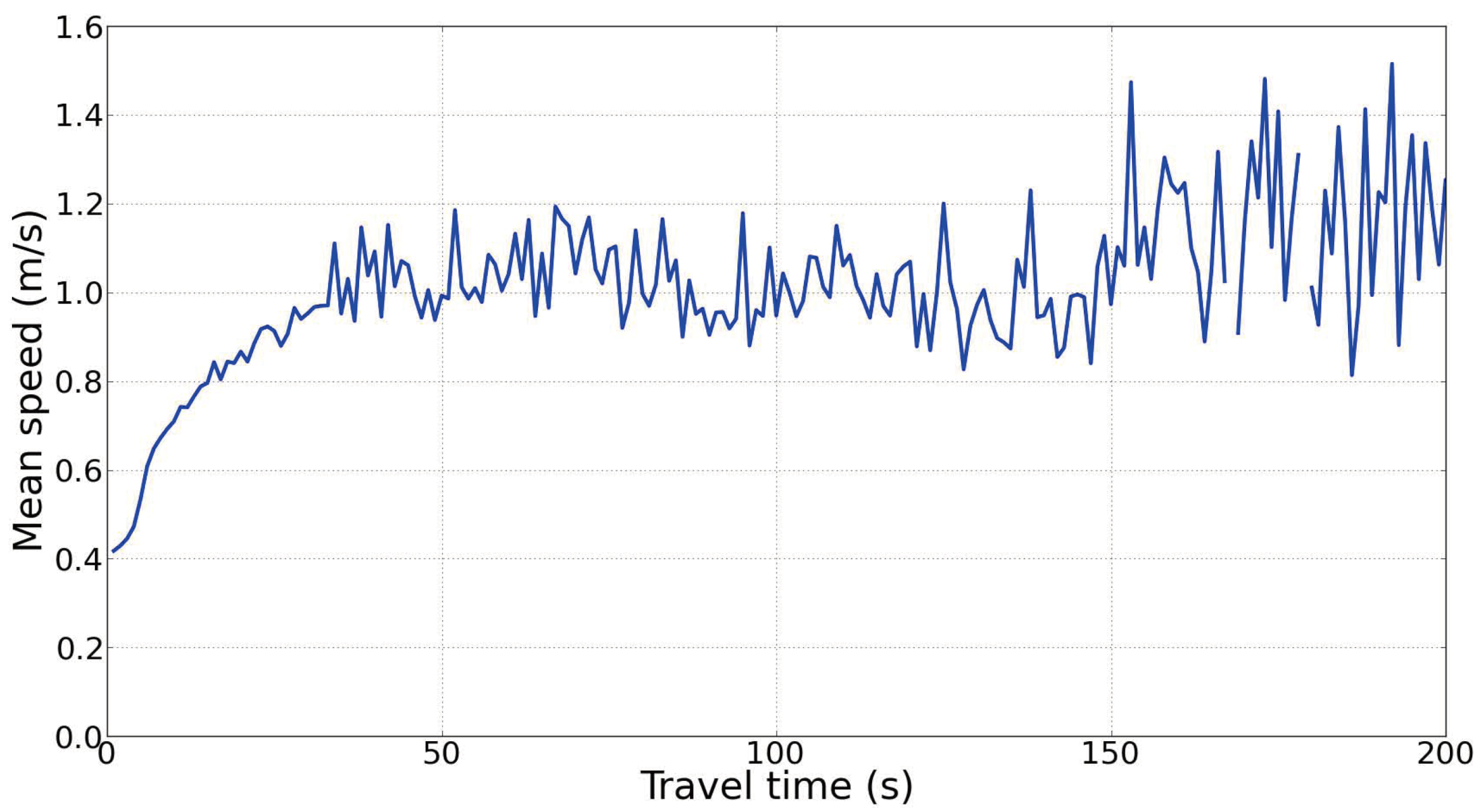
Figure 9 sheds more light on the sharp increase in error rates beyond 30 s. Short-term movements below 30 s in duration typically occur at relatively low speeds between 0.4 and 1 m/s. In contrast, the nodes move at speed regularly exceeding 1 m/s for longer term movements. Keeping the accelerometer off for a duration within 30 s thus strikes a suitable balance between energy efficiency and a tolerable increase in position uncertainty. We select
![Jsan 01 00183 i017]()
as 30 s for the remainder of the paper.
Figure 9.
Mean speed as a function of travel time. Movement of duration shorter than 30 s occurs with lower speeds, which limits the increase of position errors when TM is within 30 s.
Figure 9.
Mean speed as a function of travel time. Movement of duration shorter than 30 s occurs with lower speeds, which limits the increase of position errors when TM is within 30 s.
While the algorithm is in stationary mode, we enforce a slow increase in uncertainty to account for slow movements of the nodes that are below the speed threshold. The rate of uncertainty increase is highly specific to the mobility features of the tracked entities.
Figure 10 illustrates the distribution of the movement distance of all nodes in the cattle dataset over a 10 s time window. The results show that the majority of slow movements occur at a rate of less than 1 m per 10 s, or less than 0.1 m/s.
Figure 10.
Distribution of travelled distance in a 10 s time window by all nodes in stationary mode.
Figure 10.
Distribution of travelled distance in a 10 s time window by all nodes in stationary mode.
The impact of
![Jsan 01 00183 i012]()
is shown in
Figure 11. The X-axis shows the uncertainty increase in meters for every 10 s interval, so a value of 0.1 m corresponds to an assumed stationary speed
![Jsan 01 00183 i012]()
of 0.01 m/s. The results show that a value of
![Jsan 01 00183 i012]()
of 0.04 m/s provides the most energy-efficient configuration within the 5% error tolerance of our application.
Figure 11.
The effect of varying
![Jsan 01 00183 i012]()
. Lower values reduce the GPS duty cycle, as the uncertainty reaches AAU less often, yet increase the error rate. Higher
![Jsan 01 00183 i012]()
deliver a 66% decrease in positioning errors at a slightly higher power consumption for added GPS locks.
4.4.2. Motion State
The two main parameters of interest in the motion state are the length of the minimum rest time
![Jsan 01 00183 i026]()
and the accuracy of the accelerometer in detecting the stationary state.
While in the motion state, the node duty cycles its accelerometer by checking for motion every
![Jsan 01 00183 i026]()
to check if the node has transitioned into the stationary state.
Figure 12 shows the performance of our duty cycling strategy for different values of
![Jsan 01 00183 i026]()
. The results show that a minimum stationary time of 10 s yields the best trade-off within the 5% error tolerance. An unexpected result is that duty cycling the accelerometer in the motion state almost always provides fewer positioning errors relative to keeping the accelerometer always on while in this state. This stems from the noisy outputs of the accelerometer. If it remains on in motion state, it is more susceptible to jittery effects that point to false motion, which results in the accelerometer remaining in the motion state for longer. By switching off for a few seconds, the accelerometer achieves a form of temporal sampling diversity, so that the next sample is less correlated with the current sample, which helps to more accurately capture the true state of the device.
Figure 12.
The effect of varying the minimum stationary time
![Jsan 01 00183 i026]()
. A 10 s off-time for the accelerometer yields the lowest error rates and power consumption.
Figure 12.
The effect of varying the minimum stationary time
![Jsan 01 00183 i026]()
. A 10 s off-time for the accelerometer yields the lowest error rates and power consumption.
Another consideration is the length of time that a node in motion state checks its accelerometer for detecting a switch to stationary state
![Jsan 01 00183 i011]()
.
Figure 13 shows that longer check times are more robust to transient noisy readings due to their time averaging feature. However, a 1 s check for non-motion is sufficient to deliver our application error tolerance and provides the best energy consumption.
4.5. Summary
In this section, we have introduced and evaluated an algorithm for duty cycling the accelerometer module on a mobile node based on local information only. We have also explored the design space for this algorithm and established the suitable parameter settings for our target scenario of energy efficient localisation within an error tolerance of 5%. The next section will use this configuration to propose group based duty cycling of accelerometers.
Figure 13.
The effect of varying the accelerometer check time
![Jsan 01 00183 i011]()
. A longer check time yields more accurate results as it reduces the effects of noise.
Figure 13.
The effect of varying the accelerometer check time
![Jsan 01 00183 i011]()
. A longer check time yields more accurate results as it reduces the effects of noise.
5. Collaborative Localisation
The key idea of our collaborative localisation method is that groups of nodes that are known to cluster together can share the burden of motion detection. When operating individually, nodes use their motion detection modules to detect motion events and trigger the GPS module to activate. While nodes can cooperate through periodic contact logging, they set their accelerometer duty cycles individually.
In collaborative localisation, nodes can significantly reduce their motion module duty cycle proportionally to the size of the group. To achieve this, each node keeps track of its neighbourhood through periodic contact beacons of period (P), maintaining a neighbour table that maps each neighbour’s ID to its probability of contact with the local node over a recent time window of length (T) seconds. Each node considers all neighbours that have been regularly in close contact with it (nodes whose probability of contact is higher than a given proximity threshold) to be part of the same group or community. Once nodes know their group membership and size, it is highly likely that the decision by one node to move will be highly correlated with the movement decisions of other nodes in the same group. For a group of
G nodes, each node can set its duty cycle to
![Jsan 01 00183 i027]()
. In other words, nodes in group
G can reduce their duty cycle by a factor of the group size |
G |.
5.1. Characterising Clusters
The utility of collaborative localisation depends highly on the clustering dynamics of the monitored individuals. Individuals whose movement is tightly coupled will benefit more from collaborative localisation than individuals that move independently of others. This paper defines clusters according to spatial proximity: nodes that are within a certain distance R of each other for at least T seconds are part of the same cluster. Naturally, clusters vary over time depending on the movement of the constituent individuals.
We define a boolean instantaneous proximity function:
Instantaneous proximity estimates can be highly noisy due to signal variations and for nodes at the boundary of the proximity radius. Localisation estimates, particularly those based on GPS, can be noisy and unreliable for single samples, and they tend to be more reliable when taken over several samples. These variations emphasise the need for capturing proximity over a time window rather than a single sample. Extending γ for a time window of n discrete time samples T = T1…Tn yields:
This function returns a value between 0 and 1 that represents the proportion of samples in window T during which nodes Ni and Nj are within the proximity radius R. A proximity of 1 over a time window means that the two nodes have been within a radius R for the whole duration of the time window. Similarly, a γT of 0 means that the nodes are beyond the proximity radius for the whole duration of the time window.
The selections of R, T and the minimum threshold γT that governs cluster membership clearly have a direct impact on proximity. Larger proximity radii deliver large cluster memberships, while larger time windows and threshold γT provide more stable clusters. Both of these effects are desirable for collaborative localisation. However, both of these values involve inherent trade-offs. Using excessively high proximity radii for collaborative localisation means that nodes have to rely on cluster members that are farther away, which reduces the localisation accuracy. Similarly, time windows that are too long or γT thresholds that are too high can lead to smaller clusters because of their proximity requirement for a longer duration, which reduces the benefits of collaborative localisation.
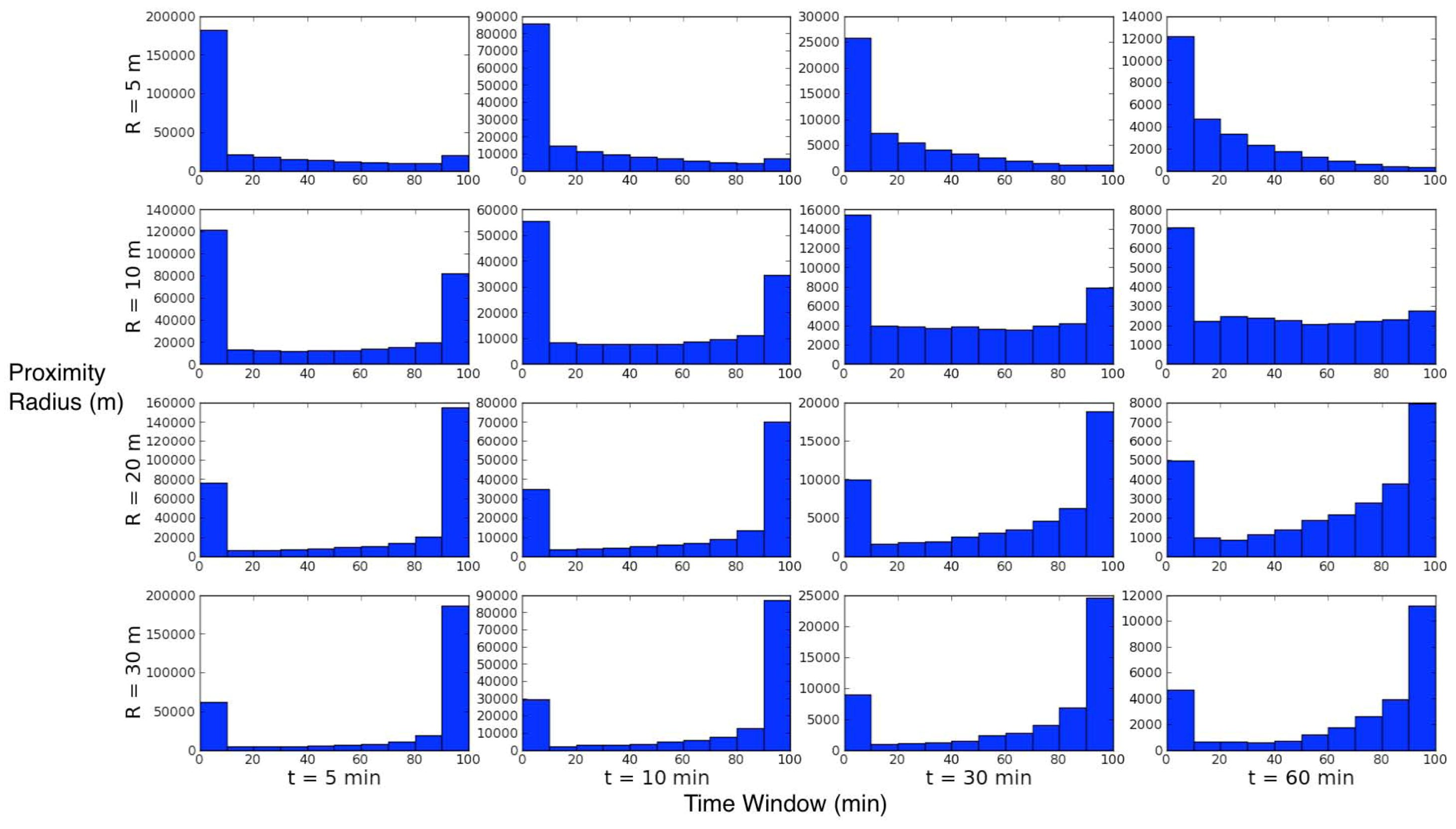
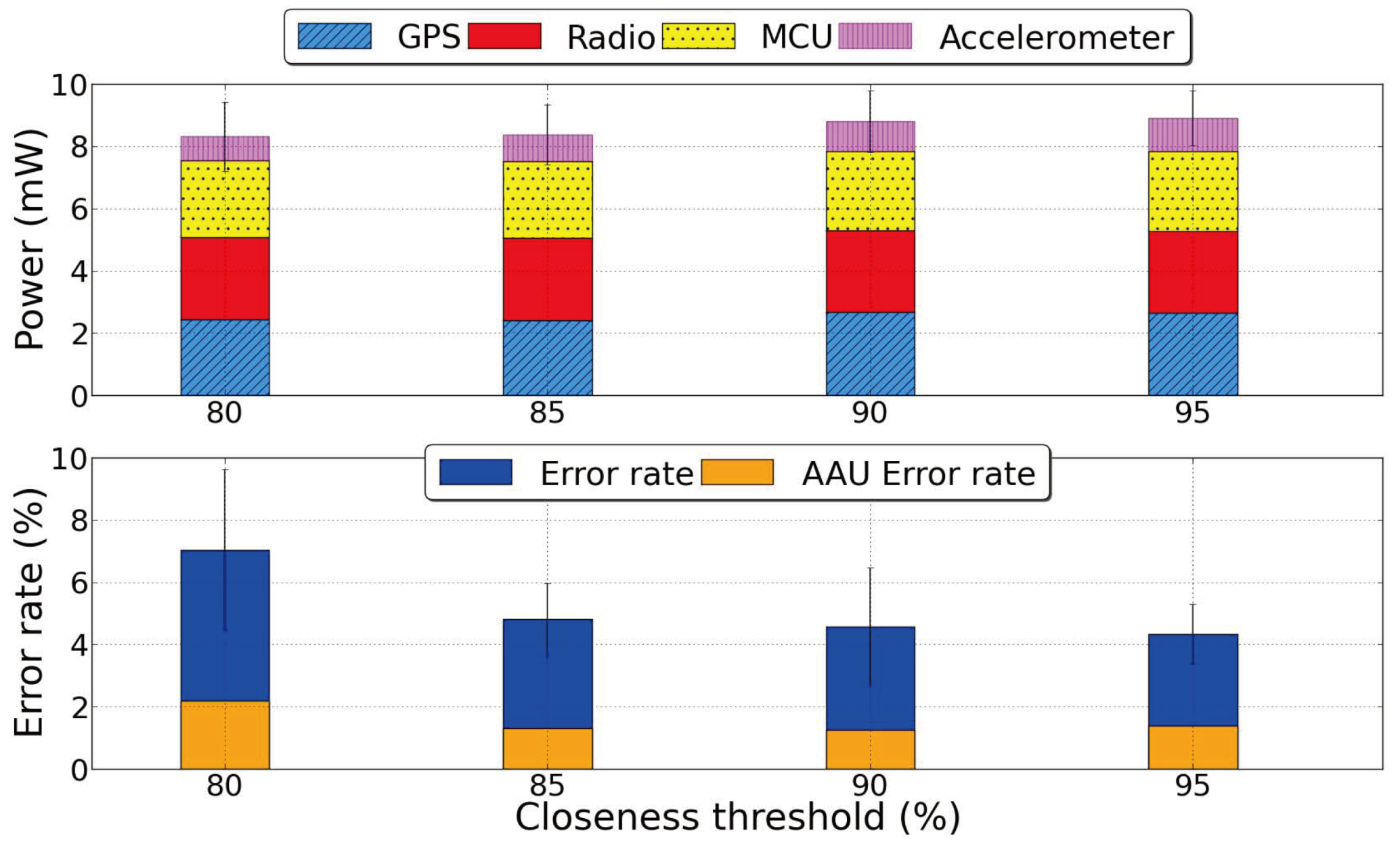
We now explore these effects on our cattle dataset. In order to clearly separate transient and strong proximity, we are seeking proximity distributions that are well segmented. To that end, we run 16 analysis scenarios evaluating a range of values for the proximity radius R = 5, 10, 20, 30 m and for the time window length T = 5, 10, 30, 60 min. Each scenario runs through the entire datasets and determines the pairwise node proximity values for the given R and T settings.
Figure 14 shows the results of each of the radius threshold and time window value. Each row corresponds to one setting of the proximity radius
R and each column corresponds to one setting of the time window. Each plot in the figure shows the histogram of
γT values for the corresponding values of
R and
T.
As expected, a large proximity radius (20–30 m) and a short time window (5–10 min) provide the best segmentation. These settings also provide a high proportion of instances with very high proximity. At first glance, this is highly desirable. The following sections explore the effect of large proximity radii on collaborative localisation.
Figure 14.
The joint impact of the proximity radius R and the time window T.
Figure 14.
The joint impact of the proximity radius R and the time window T.
5.2. Collaborative Duty Cycling
The main concept of collaborative duty cycling is to share the burden of motion detection among a group of nodes whose movement appears closely interdependent. To detect a motion event while the group is in a stationary state, at least one of the nodes in the group must sample its accelerometer during the event. Because motion events persist for at least
TM, at least one node in the group must sample its accelerometer every
![Jsan 01 00183 i017]()
seconds. With
G nodes in the group, each node can power off its accelerometer for
![Jsan 01 00183 i028]()
seconds. Note that we only rely on collaborative duty cycling in the stationary state. When nodes are in the motion state, they revert to individual duty cycling.
Figure 15 shows a typical motion detection time line with our group based duty cycling algorithm.
Figure 16 illustrates how collaborative duty cycling of accelerometers works alongside GPS duty cycling. All nodes send periodic radio beacons that contain their uncertainty and current number of neighbours, with period
TR, to maintain neighbourhood state. Each node maintains a neighbourhood table where it stores the proportion of neighbour beacons received in the recent time window
T. Periodic beacons also serve the purpose of limiting neighbour uncertainty, as in [
5]. Nodes that receive a beacon from a neighbour with a lower uncertainty can reduce their own uncertainty by using that neighbour as a reference.
Whenever a node obtains position lock from GPS, it samples its accelerometer for
![Jsan 01 00183 i010]()
seconds. If it detects no motion during that period, the node transitions into stationary state. At this point, the node determines its
true neighbours, which are the nodes in its neighbourhood table for which the node has received at least
δ beacons in the past
T seconds. The
δ parameter is a tunable proximity threshold that defines the degree of level of proximity that provides a suitable degree of confidence in neighbour movement correlation.
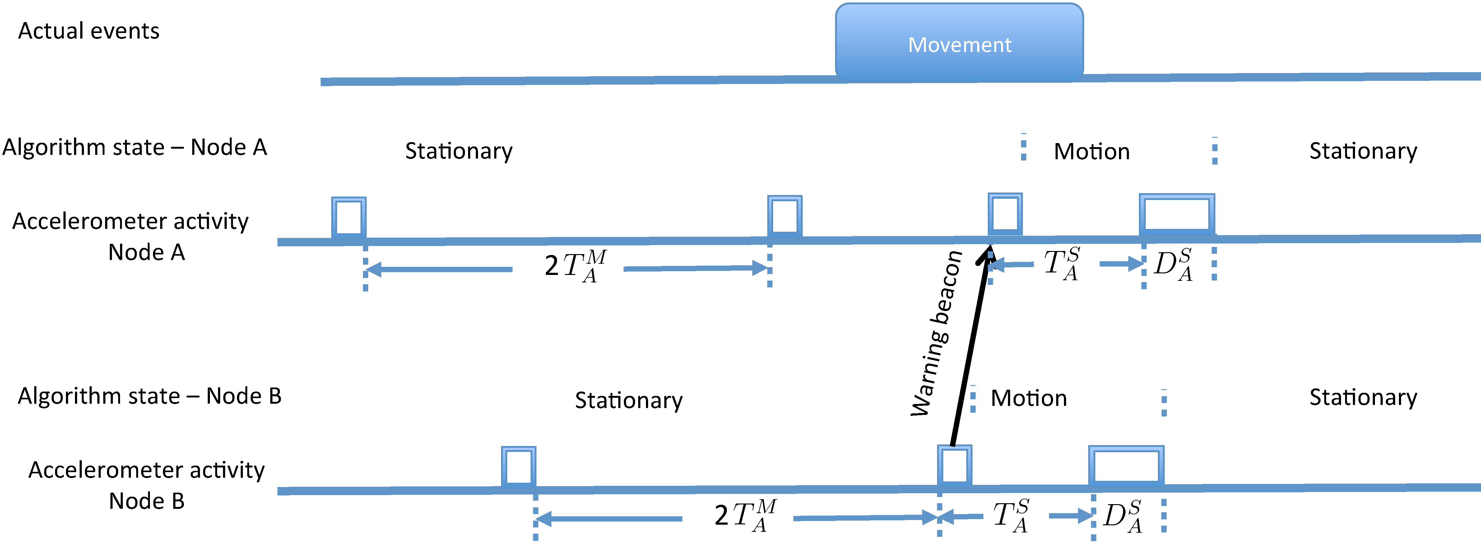
Figure 15.
Group-based Accelerometer Duty Cycling showing a timeline of actual motion events, algorithm state, and the active/sleep periods of the accelerometer for two nodes A and B. Initially, both nodes are in stationary state and their accelerometers are duty cycled with a period of
![Jsan 01 00183 i029]()
. Once node B detects motion, it sends a warning beacon to node A and switches to the motion state. When node A receives the warning beacon, it samples its accelerometer and detects that it is moving, so it also switches to its motion state.
The node also considers the number of neighbours of all of its true neighbours (recall that each node embeds its number of true neighbours in periodic beacons) and selects
G =
min(
G(
N)), where
G(
N) is the number of true neighbours of neighbor
N. This step is required to ensure consistency in accelerometer duty cycling among nodes in the same group, when some of the nodes belong to overlapping groups of nodes. The node can then set its own duty cycle locally as
![Jsan 01 00183 i030]()
. The reasoning is that each of the node’s true neighbours will run the same local computation and set at least the same duty cycle (depending on their neighbours’ number of neighbours). Determining true neighbours and setting the collaborative accelerometer duty cycle repeats at every time step while the node is in stationary state to ensure adaptation to neighbourhood changes.
Whenever any node samples its accelerometer and detects movement at a speed above
![Jsan 01 00183 i006]()
, the node leaves the stationary state and broadcasts a
warning beacon to all of its neighbours. All neighbours that receive the warning beacon sample their accelerometer immediately to determine if they too have started moving. If so, the neighbours also enter the motion state, and otherwise, they stay in the stationary state.
Nodes that enter the motion state increase their uncertainty by
![Jsan 01 00183 i031]()
, as in the individual duty cycling case. As long as their uncertainty has not reached the critical limit of
AAU −
tL, they duty cycle their accelerometer less aggressively with an off time of
![Jsan 01 00183 i026]()
and update their uncertainty every time instance by
![Jsan 01 00183 i013]()
. If the uncertainty reaches the critical limit, the node powers on its GPS for a new position estimate. If the node powers on its accelerometer before the uncertainty reaches the critical limit and detects no motion for at least
![Jsan 01 00183 i011]()
seconds, it transitions back into stationary state.
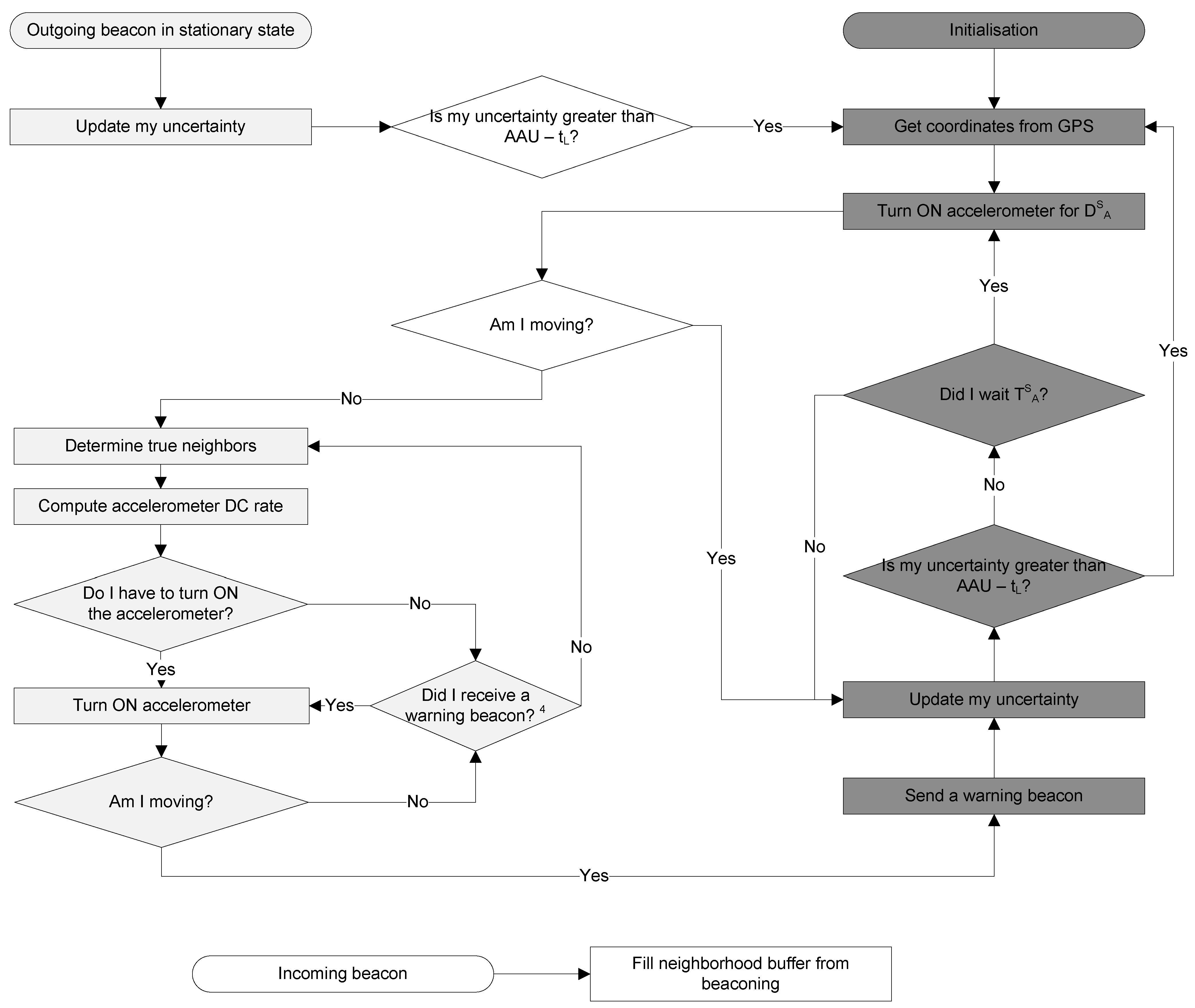
Figure 16.
A flowchart of the group-based duty cycling strategy. The white and dark shaded blocks refer to the stationary and motion states respectively.
Figure 16.
A flowchart of the group-based duty cycling strategy. The white and dark shaded blocks refer to the stationary and motion states respectively.
5.3. Example
Figure 17 shows a trace of the uncertainty growth for 3 nodes from our empirical cattle dataset. The trace uses solid lines to indicate the algorithm uncertainty and dashed lines to indicate the true error for each node. At the start of the trace, all three nodes are growing their uncertainty linearly according to
![Jsan 01 00183 i012]()
, after having logged contact with a common neighbour 104, whose trace is not shown here. At around
t = 200, node 103 detects motion through its accelerometer, which results in a step increase in its uncertainty. However, in the following time instance, node 103 logs contact again with node 104 and reduces its uncertainty again. This happens again in the next cycle with a smaller peak, as node 103 has now switched to a shorter accelerometer duty cycle in motion state. After that, node 103 detects that it has stopped moving, and reverts to slow uncertainty increase. Nodes 337 and node 103 are in the same situation at t = 1,200, 1,250 respectively. At around t = 1,225, node 299 has a sharp increase in uncertainty before node 337 obtains GPS lock and lowers its uncertainty. This is a consequence of using the dynamic speed model with step increases in uncertainty upon motion detection. The last time node 299 got GPS lock, it had a speed of 0.8 m/s. It keeps this speed estimate until its next GPS lock. When it detects motion, it adds
![Jsan 01 00183 i032]()
to its uncertainty, which causes this sharp rise. When node 337 obtains lock a few seconds later, this situation is rectified. Another node 394 (not shown here) is also nearby and obtains lock at nearly the same time. At around 1,450 s into the simulation, node 337 detects motion on its accelerometer and sends a warning beacon to its neighbours. Node 103 detects that it is also moving after sampling its accelerometer, while node 299 detects that it is not. Both nodes 103 and 337 add a step increase to their uncertainty after detecting motion. They shortly log contact with node 394 to reduce their uncertainty again. Note that the actual position error remains within the uncertainty at all times.
Figure 17.
The growth of uncertainty with collaborative duty cycling. There are fewer motion detection events with group duty cycling.
Figure 17.
The growth of uncertainty with collaborative duty cycling. There are fewer motion detection events with group duty cycling.
5.4. Parameter Settings and Trade-offs
The accuracy of partitioning nodes into groups that travel together critically influences both the power consumption and error rate metrics of the localisation algorithm. Nodes use their energy unnecessarily if triggered by a motion beacon when they are not moving. On the other hand, the localisation error rate grows when the nodes fail to update uncertainty bounds as a result of not receiving a motion beacon in the motion state.
5.4.1. Group Radius
We first explore the selection of the group radius and its effect on performance. We note here that real world deployments yield ranges that are directional as radio transmissions are severely attenuated by obstacles, such as animals’ bodies, or false positives when detecting animal movement. While this paper considers an idealised transmission radius for simplicity of analysis, the techniques presented here do not introduce additional error if our idealised assumptions are not true, but they rather decrease the performance benefits. Thus the worst case scenario is that the collaborative algorithms will have the same performance as for an individual animal not gaining any benefits from group localisation or motion detection. For example, if a node receives a warning beacon from a neighbour within
![Jsan 01 00183 i017]()
time from the last time it checked its accelerometer, it simply ignores the beacon as it is already in motion state.
The discussion above suggests that larger group radii are more favourable. However, larger radii implicitly limit the opportunity for GPS duty cycling. Whenever a node logs contact with a neighbour, it resets its uncertainty as the sum of the neighbour’s uncertainty and the proximity radius. A larger radius means that nodes will have higher uncertainty from neighbour encounters and will activate their GPS modules more often.
Figure 18 shows the effects of varying the group radius on power consumption and localisation accuracy. A group radius of 20 m or more results in high error rates since warning beacons from any neighbours will immediately increase the local node’s uncertainty by at least 20 m, with a high likelihood of exceeding the AAU of 50 m. A shorter radius of 10 m has a higher power consumption, as fewer nodes are deemed as neighbours, but it bounds the error rate within 5%.
Figure 18.
Performance with different group radius. Benefits from group-based duty cycling decrease for smaller groups.
Figure 18.
Performance with different group radius. Benefits from group-based duty cycling decrease for smaller groups.
5.4.2. Neighbour History
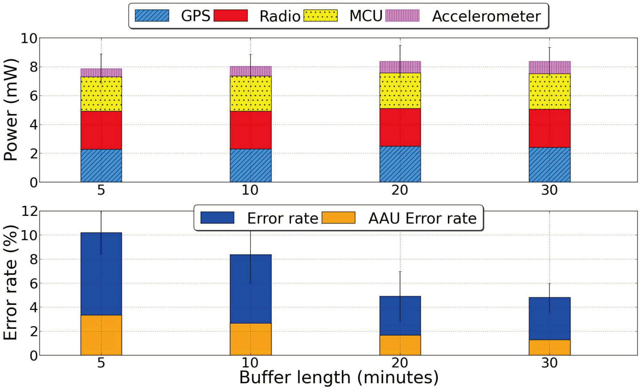
We now turn our attention towards selecting the length of the time window for maintaining neighbour history. Shorter time windows can respond quickly to neighbourhood changes, while longer time windows favour stable group memberships.
Figure 19 shows the impact of the time window length on power and localisation errors. Longer time windows clearly provide more accurate positioning for group-based duty cycling at a minor increase in power consumption. These results may stem for the nature of our cattle dataset, where group changes occur on longer time scales. The slight increase in power consumption with longer time windows is a result of an increase in the accelerometer power consumption. Because longer time windows favour stable groups, they cause neighbours that are transiently close to a node to be excluded from the node’s group. This leads to smaller average group sizes for nodes, which results in a higher accelerometer duty cycle.
Figure 19.
Performance with different sizes of neighbour history buffer. A longer buffer size of 30 minutes helps establish stable groups.
Figure 19.
Performance with different sizes of neighbour history buffer. A longer buffer size of 30 minutes helps establish stable groups.
5.4.3. Proximity Threshold
Having selected a group radius of 10 m and a neighbour history time window of 30 min, we refer back to
Figure 14. In particular, our simulations point to the plot in the second row and the third column (
R = 10 m and
T = 30 min) of that figure. We seek to select the value of the proximity threshold
δ that captures to classify true neighbours from transient ones. We are effectively aiming to draw a vertical line on the plot that separates these two classes of neighbours.
Figure 20.
Performance with different proximity threshold settings.
Figure 20.
Performance with different proximity threshold settings.
We evaluate four values for the proximity threshold between 80% and 95% in separate simulations. The resulting power consumption and error rates are shown in
Figure 20. Higher thresholds improve error rates as they are more conservative in labelling useful neighbours. They also lead to smaller groups, which reduces the savings of group-based duty cycling. We select a threshold of 85% as the most energy efficient value that meets our application’s error tolerance of 5%.
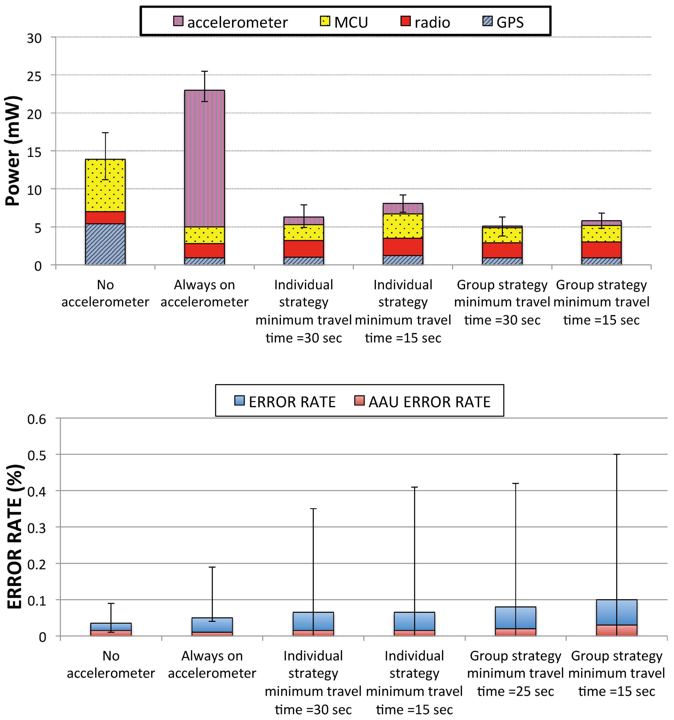
6. Performance Evaluation
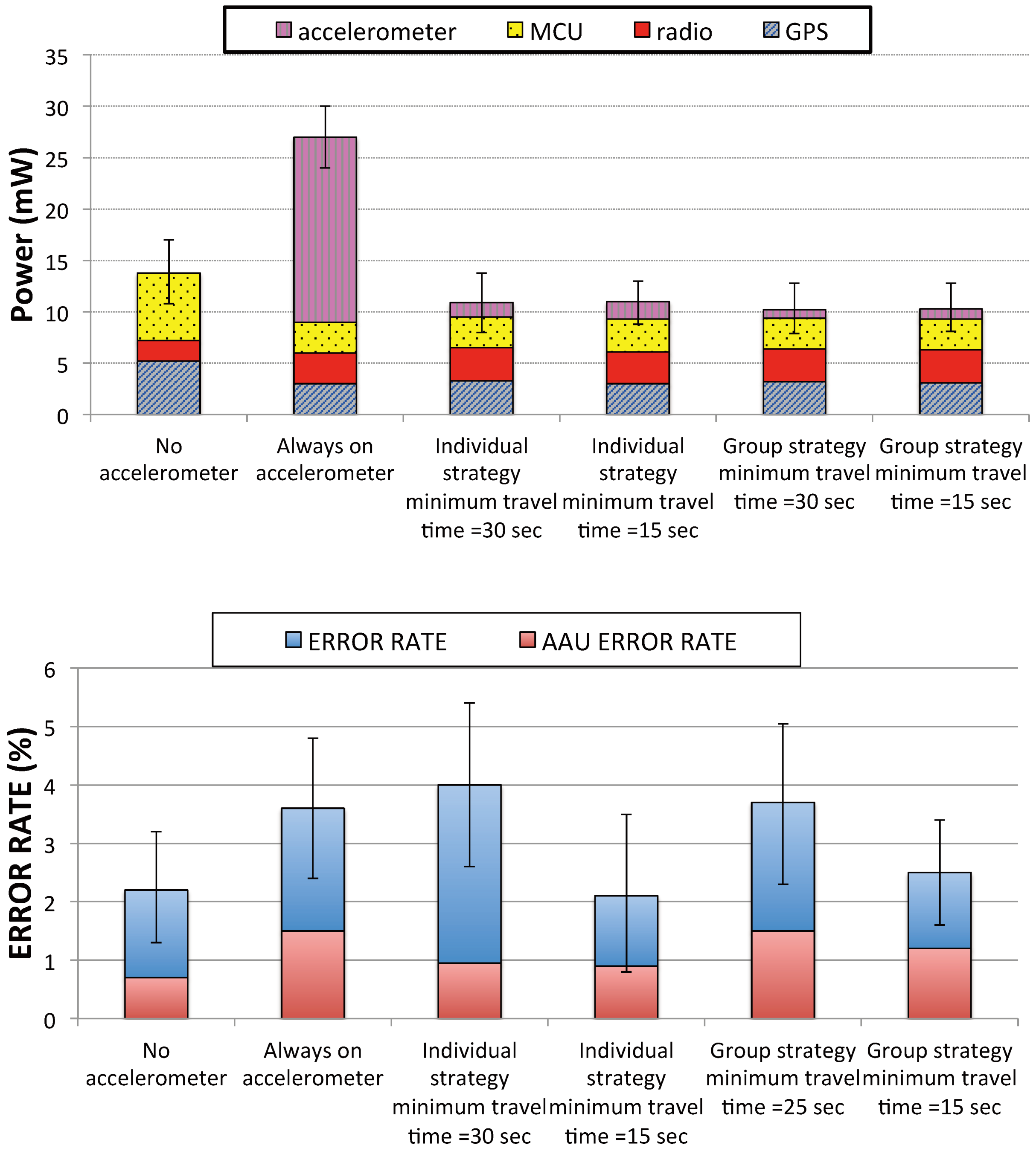
We use simulations based on the data that we empirically collected in cattle networks and evaluate performance of the individual and collaborative localisation techniques with respect to the previous GPS duty cycling algorithm and an always-on accelerometer triggering a duty cycled GPS. For the always-on accelerometer approach, we conservatively assume that the activation of the accelerometer does not contribute to an increase in the MCU duty cycle.
Due to the extensive mobility of animals in our datasets, the performance of the group-based strategy provides relatively small benefits over the individual strategy. To further quantify the effect that the group-based duty cycling might have in other potential areas of application, we also evaluate the different strategies in low mobility scenarios observed during the night, when animals are resting.
6.1. Individual vs. Collaborative Localisation
We compare the performance of individual duty cycling, group-based duty cycling with 2 baseline scenarios: (1) an always-on accelerometer that triggers a duty cycled GPS to turn on when there is motion, where radio contact logging is used for local position sharing; and (2) the previous work on GPS duty cycling and radio proximity, with no accelerometer. We run two separate sets of simulations for these approaches with different travel times, in order to illustrate how performance can be tuned to favour energy or error rate. The algorithm with no motion accelerometer uses event-based beaconing, which had been established as the most effective approach in [
5], while all other algorithms use periodic beaconing, for reasons discussed in
Section 4 and
Section 5.
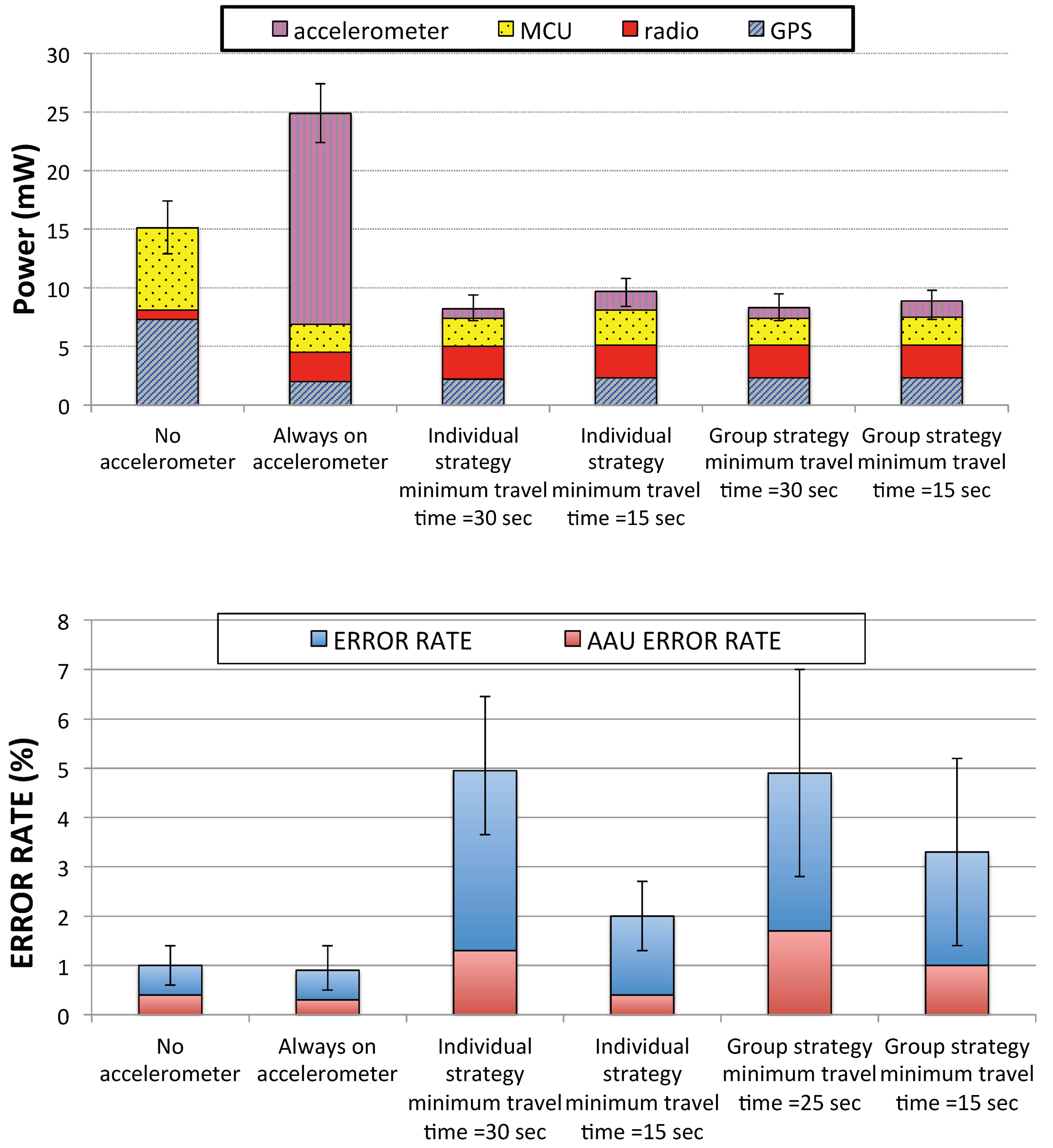
Figure 21 compares the results. Both flavours of our accelerometer duty cycling strategies reduce the power consumption by around 50% over the GPS duty cycling with radio ranging approach and 72% over the always-on accelerometer approach. This comes at the cost of an increased error rate that remains within our application’s 5% error tolerance. The higher error rate with accelerometer duty cycling is intuitive, as nodes slow down their uncertainty growth in stationary state until they detect movement. The bars for a travel time of 15 s show the performance of accelerometer duty cycling for applications with tighter accuracy constraints. This shorter
![Jsan 01 00183 i017]()
only causes minor increases in power consumption (about 1 mW for individual duty cycling and less than 0.5 mW for collaborative), while reducing their error rates to 2% and 3.5% respectively. Group duty cycling saves about 10% in power consumption over individual duty cycling, as nodes can set longer accelerometer off time. This comes at an increase of 1.25% to the error rate, since the longer accelerometer off times increases the likelihood of missed motion events.
Figure 21.
Performance comparison of the three strategies over the entire dataset.
Figure 21.
Performance comparison of the three strategies over the entire dataset.
Notably, the algorithm with no accelerometer consumes significantly higher energy for powering the GPS module and the MCU, while consuming less than half the energy for radio communication. The higher GPS power consumption is clearly because of the more frequent GPS fixes in the absence of accelerometer triggering. The MCU power consumption is also higher because the MCU has to remain active while the GPS is powered on (see overlap parameter in energy model). The radio power consumption is lower for this algorithm as it uses event-based beaconing, while both individual and group-based duty cycling use periodic beaconing. The results clearly show that the added cost of periodic beaconing is well worth the savings in GPS and MCU power consumption, which result from a significant decrease in the frequency of GPS fixes.
While keeping the accelerometer always on to trigger GPS position locks does reduce GPS power consumption thanks to a reduced frequency of locks, it is the most energy-expensive option, as the accelerometer module consumes 18 mW to power up its tilt compensation and heading calculations in hardware. This algorithm also results in the best location accuracy, slightly outperforming the no-accelerometer algorithm due to more adaptive GPS locks.
6.2. Mobility Dependencies
This section examines the performance dependence of our duty cycling strategies on the degree of mobility.
Figure 22.
Power consumption and accuracy for the 3-hour interval in the data trace with the highest number of motion events.
Figure 22.
Power consumption and accuracy for the 3-hour interval in the data trace with the highest number of motion events.
We first evaluate the effectiveness of our duty cycling strategies for highly mobile scenarios. We select the 3-hour time window from the data trace with the highest number of motion events, and we run each of the duty cycling strategies for all the nodes during that time window only. The results are shown in
Figure 22. Both individual and group-based accelerometer duty cycling strategies reduce the power consumption relative to GPS duty cycling with radio proximity (between 21% and 35% respectively) and relative to the always-on accelerometer (between 60% and 62% respectively), at the cost of increased error rates as they use accelerometer estimates to reduce reliance on GPS. Both approaches deliver comparable error rates with GPS duty cycling while delivering this energy benefit. For the group-based strategy, a 30 s
![Jsan 01 00183 i017]()
caused the error rates to go above the error tolerance, so we show here the results for
![Jsan 01 00183 i017]()
of 15 s and 25 s for that strategy. The individual accelerometer duty cycling approach outperforms the always-on approach, indicating that duty cycling the accelerometer can lead to fewer false positives in detecting transient motion.
Figure 23.
Power consumption and accuracy for the 3-hour interval in the data trace with the fewest number of motion events.
Figure 23.
Power consumption and accuracy for the 3-hour interval in the data trace with the fewest number of motion events.
Next, we explore the case of rare movement events. We select the 3-hour time window from the data trace with the least number of motion events, and we run each of the duty cycling strategies for the all the nodes during that time window only. The results are shown in
Figure 23. Both individual and group-based accelerometer duty cycling strategies significantly outperform GPS duty cycling with radio proximity (50%–65%) and the always-on accelerometer (65%–78%) in terms of power consumption, with a modest increase in error rates that remains well within the application-specific limit of 5%. The group-based approach delivers a further 20% improvement in power consumption over individual duty cycling, as the nodes that share the accelerometer sampling burden get to spend a longer time in off mode. Interestingly, a
![Jsan 01 00183 i017]()
of 30 s yields the best results for low mobility, as it is less likely to miss motion events during the longer accelerometer sleep time. GPS duty cycling with radio ranging delivers the highest accuracy, outperforming the always-on accelerometer. All versions of accelerometer duty cycling exhibit slight reductions in accuracy, while staying well within the 5% error tolerance.
6.3. Summary
The results in this section have shown that while both flavours of accelerometer duty cycling improve the power consumption over previous work, sharing the burden of duty cycling among members of a group is beneficial primarily in situations where the expected likelihood of motion is relatively low. When that is not the case, performance of the two approaches is comparable with a slight improvement in error rate for the individual approach.
7. Discussion
7.1. Mobility Pattern Adaptation
The results have shown that individual accelerometer duty cycling performs better during high activity time windows, and that collaborative localisation performs better during low activity time windows. This effect stems from the highly deterministic and synchronous nature of individual duty cycling. For the same reason that synchronous MAC protocols perform better with high traffic scenarios, individual duty cycling is well-suited for situations where the likelihood of a motion event is high. The reason that it outperforms collaborative duty cycling in this situation is that the latter distributes the burden of activity check across multiple neighbours, some of which may leave the group during critical times.
Through similar reasoning, collaborative duty cycling performs well under low activity scenarios as the dynamic nature of moving nodes adds a randomisation effect to the sample schedules. This randomisation is beneficial for detection of motion events in the group, whose distribution in non-deterministic.
An interesting extension of our work is to enable nodes to adapt their accelerometer duty cycling strategy based on their observed motion levels. When the frequency of motion events exceeds a certain threshold, nodes switch to individual duty cycling. When activity slows down, they can revert to collaborative duty cycling. The results in
Figure 22 and
Figure 23 suggest that additional savings can be achieved by actively enforcing this strategy.
7.2. Group Overlaps
The group structure across a dynamic topology of mobile nodes will almost certainly lead to asymmetric views of groups among nodes. For instance, a node A may have ten neighbours, nine of which are tightly connected and have a consistent view of their group. These neighbours can simply set an accelerometer duty cycle at one-tenth of their individual duty cycle. Node A’s tenth neighbour, node B, only sees node A as its neighbour, because it is further away from the other nodes in the group. As a result, node B sets its duty cycle at 50% of its individual duty cycle. Node A will also set its duty cycle to 50% of the individual duty cycle, thanks to the min(G(N)) operation through which it can accommodate its least connected neighbour. This approach also holds true in the case of multiple group overlaps.
7.3. Desynchronisation
Another issue is whether group members are implicitly synchronised through warning beacons, and whether this has an impact on the performance of our collaborative duty cycling strategy. A few features in our algorithms help avoid implicit synchronisation. Firstly, nodes notify neighbours when getting GPS lock, which avoids race conditions for this operation. Second, nodes in overlapping groups will check their accelerometers at different intervals, which contributes to desynchronisation. Additionally, the use of the dynamic speed model leads nodes to grow their uncertainties at different rates in motion states, helping to avoid implicit synchronisation. Finally, the specific individual movement or non-movement patterns also help desynchronisation of uncertainty growth. A node in a group that detects movement at one instance will trigger a warning beacon to neighbours. A subset of neighbours will switch to motion state if they are moving as well. This will cause desynchronisation among nodes in the moving subset and the rest of the group. At another point during the process, another subset of the group may similarly detect motion and shift their uncertainty growth away from the rest of the group.
7.4. Advanced Mobility Models
This paper has considered a simple mobility model for the animals consisting of a stationary and moving state. While this model can easily be generalised to other moving objects, more fine-grained modelling of the motion states can potentially yield improved accuracy and energy efficiency. In the case of cows, previous studies suggest that motion can be modelled using three [
27] or four states [
28]. The potential benefits of more fine-grained motion modelling should be weighed against the ability of motion detection modules to accurately distinguish between the states. This remains an open issue for future work.
7.5. Empirical Validation
The group based motion detection algorithms in this paper have used empirical data traces to explore the design space and establish the utility of this approach, particularly when the mobile entities move rarely. An interesting direction for future work would be to empirically test this approach in order to better quantify its benefits for real-time tracking. Empirical validation would require the use of cameras with targeted image processing algorithms for cattle tracking or through human observers for the duration of the experiment, which would limit the duration or spatial scale of the experiment.


 where DCx is module x’s duty cycle, and
  is the power consumption of that module in active mode. Both modules are completely powered off when not in use, so they draw no current. We track the radio energy consumption as the sum of the transmission, reception, and listening energy values respectively [25] for a given radio duty cycle, which is set to 10% in the rest of the paper (note that we do not consider radio state transition times in this paper for simplicity).
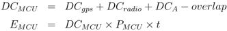


 seconds in StS, where ε is a positive small number. Similarly, the accelerometer will detect a node being stationary if it turns on once every
  seconds in the motion state StM.
 and
and  seconds, respectively. The accelerometer detects motion or non-motion by checking the amplitude of its measured signal with a predefined threshold. Nodes increase their uncertainty in both states. In the stationary state, we increase uncertainty assuming that a node is moving at a slow
  speed. This allows us to account for slow movement events such as cattle feeding, where a node moves slower than the threshold
  . Finally, a node also updates its uncertainty when transitioning to the StM state:
 is the current speed estimate and
  is proportional to the minimum travel time
  . λ is a constant between 0 and 1. For a conservative uncertainty estimate, the node sets
  , assuming the worst case scenario that the node missed the first
  , as the length of time that has already passed for the motion event is a uniformly distributed value between 0 and
  as long as motion continues and increases uncertainty accordingly. Every time instant that it increases its uncertainty, the node checks whether the uncertainty has reached a critical threshold by calling the Check_GPS() function (see Figure 4). If so, the node activates its GPS module to start the GPS lock process and powers off its accelerometer.
 . The function Set_Acc_DC() (see Figure 5) determines the suitable off time for the accelerometer for both motion and stationary states. This will depend on the current value of the node’s uncertainty. Note that a node must power on its GPS module at least tL seconds prior to its uncertainty reaching AAU, in order to account for the uncertainty growth during the GPS lock process. If a node’s uncertainty is much lower than this bound, then it can set its sleep time to TA. However, if a node that is duty cycling its accelerometer detects motion when its uncertainty is slightly below or exactly AAU-
  , then it must increase its uncertainty by
  , resulting in an uncertainty of
  . Even if the node powers on its GPS module at this instant, it is likely to have an uncertainty that exceeds AAU by the time it gets GPS lock. To avoid this situation, a node checks whether its uncertainty is greater than
  . If so, the node anticipates that it may have to incorporate a step increase in its uncertainty when it detects motion, so it sets an instantaneous value of TA to ensure that it will power on its GPS module at the right time:
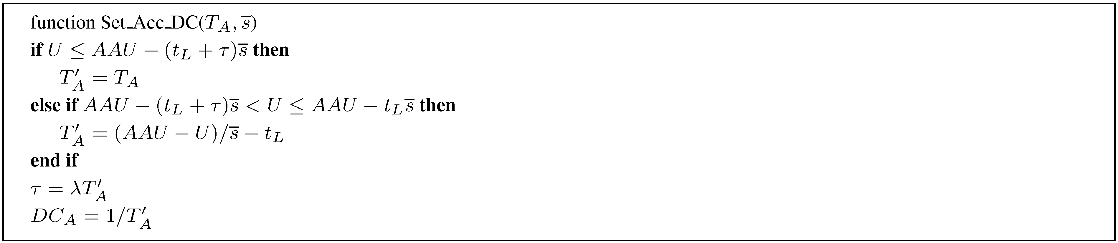
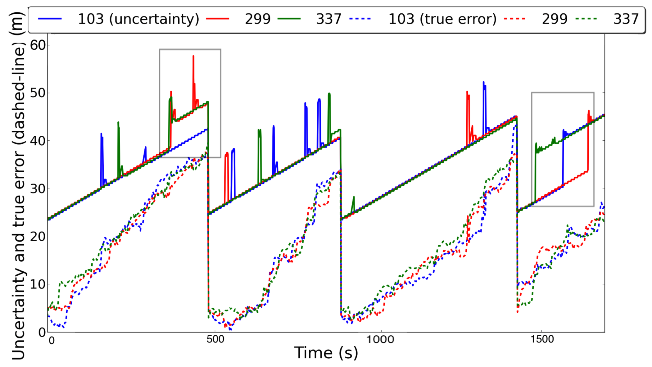


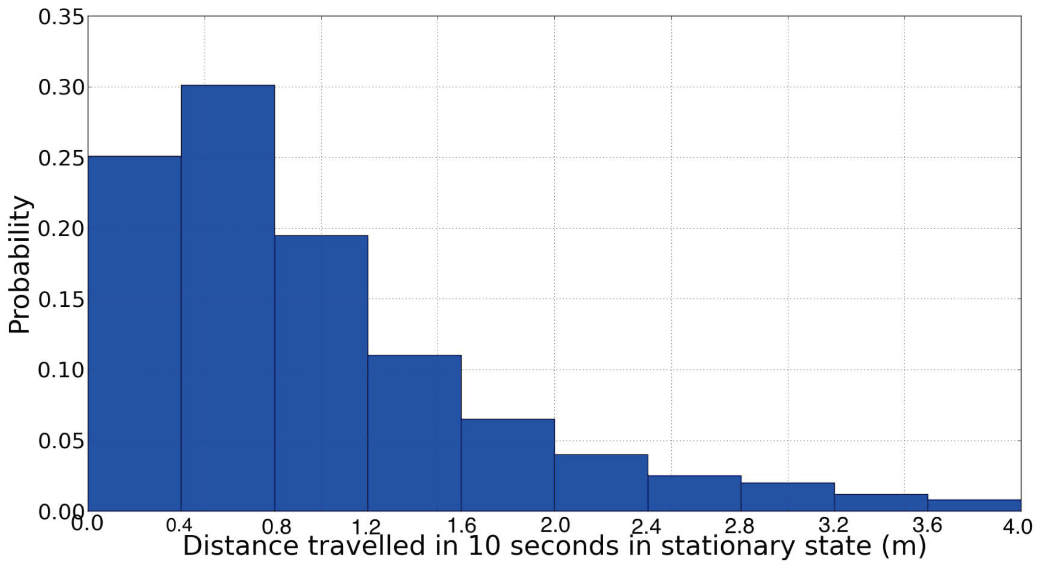
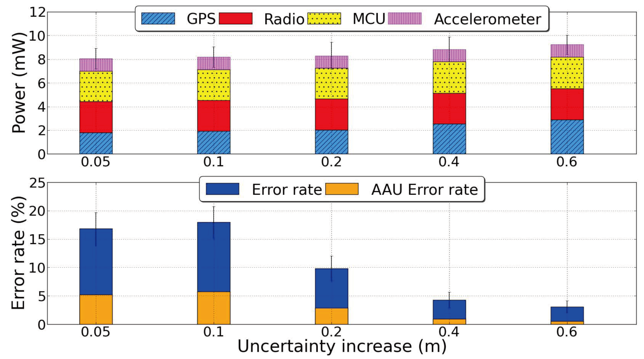
 and the accuracy of the accelerometer in detecting the stationary state.
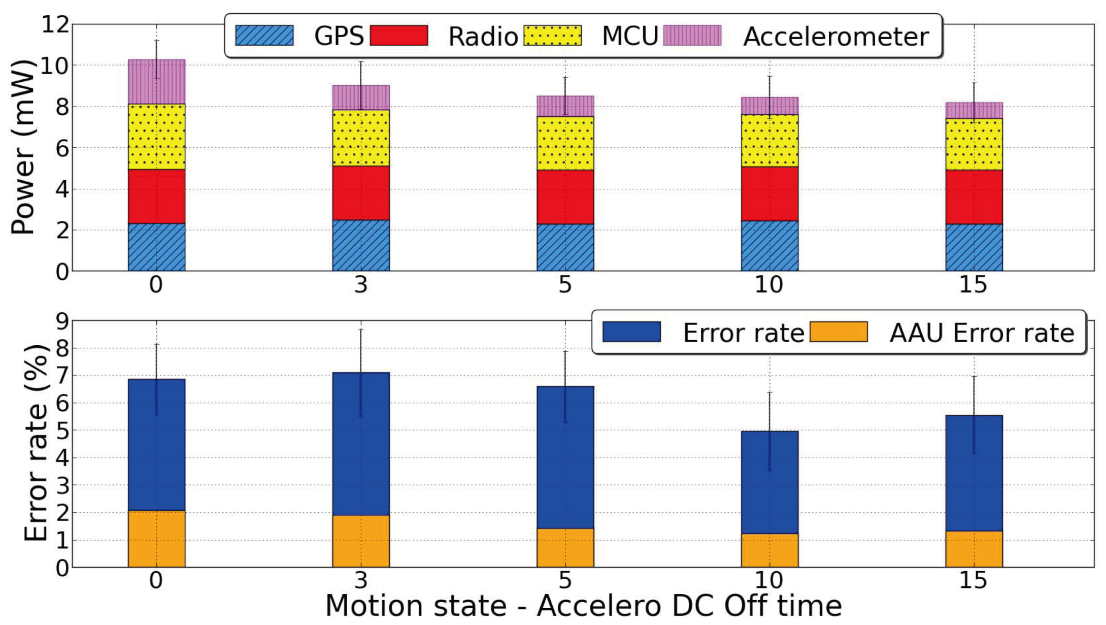

 . In other words, nodes in group G can reduce their duty cycle by a factor of the group size | G |.


 seconds. Note that we only rely on collaborative duty cycling in the stationary state. When nodes are in the motion state, they revert to individual duty cycling. Figure 15 shows a typical motion detection time line with our group based duty cycling algorithm.
 . Once node B detects motion, it sends a warning beacon to node A and switches to the motion state. When node A receives the warning beacon, it samples its accelerometer and detects that it is moving, so it also switches to its motion state.

 . The reasoning is that each of the node’s true neighbours will run the same local computation and set at least the same duty cycle (depending on their neighbours’ number of neighbours). Determining true neighbours and setting the collaborative accelerometer duty cycle repeats at every time step while the node is in stationary state to ensure adaptation to neighbourhood changes.
 , as in the individual duty cycling case. As long as their uncertainty has not reached the critical limit of AAU − tL, they duty cycle their accelerometer less aggressively with an off time of
 to its uncertainty, which causes this sharp rise. When node 337 obtains lock a few seconds later, this situation is rectified. Another node 394 (not shown here) is also nearby and obtains lock at nearly the same time. At around 1,450 s into the simulation, node 337 detects motion on its accelerometer and sends a warning beacon to its neighbours. Node 103 detects that it is also moving after sampling its accelerometer, while node 299 detects that it is not. Both nodes 103 and 337 add a step increase to their uncertainty after detecting motion. They shortly log contact with node 394 to reduce their uncertainty again. Note that the actual position error remains within the uncertainty at all times.