FLEHAP: A Wind Powered Supply for Autonomous Sensor Nodes

Abstract

The development of the Internet of Things infrastructure requires the deployment of millions of heterogeneous sensors embedded in the environment. The powering of these sensors cannot be done with wired connections, and the use of batteries is often impracticable. Energy harvesting is the common proposed solution, and many devices have been developed for this purpose, using light, mechanical vibrations, and temperature differences as energetic sources. In this paper we present a novel energy-harvester device able to capture the kinetic energy from a fluid in motion and transform it in electrical energy. This device, named FLEHAP (FLuttering Energy Harvester for Autonomous Powering), is based on an aeroelastic effect, named fluttering, in which a totally passive airfoil shows large and regular self-sustained motions (limit cycle oscillations) even in extreme conditions (low Reynolds numbers), thanks to its peculiar mechanical configuration. This system shows, in some centimeter-sized configurations, an electrical conversion efficiency that exceeds 8% at low wind speed (3.5 m/s). By using a specialized electronic circuit, it is possible to store the electrical energy in a super capacitor, and so guarantee self-powering in such environmental conditions.

1. Introduction

Internet of Things (IoT) is the next big evolution of electronics. It is based on the concept of omnipresent connectivity among different objects which in a large part are networks of wireless sensors (NWS). Such a complex system requires sensors, microcontrollers, and radio devices enabling the transmission of the collected information to the Internet (the Cloud). These sensors cannot be wired, especially when the network is intended to be used on very large areas or placed in difficult-to-reach places (i.e., buried or in harsh or hazardous locations). A common solution is to provide all nodes of the network with their own energy source, usually a battery; however, for a large number of application domains, a battery is not a reliable solution, either. In fact, installation and replacement costs can become too high if the network involves hundreds or thousands nodes. For this reason, the possibility for an application to stay reliable and economically viable on the long term (10 years or more) will more and more depend on the node’s capability to recover energy from the node’s environment, (energy harvesting, EH), either to prevent the battery from discharging or, even better, to get rid off the battery itself. Among other available sources (mechanical vibrations, light, temperature difference, etc.), a fluid in motion (air, water) can represent a useful resource of energy if a specialized device is constructed.

1.1. Methods for Harvesting Energy from Wind

Windmills and turbines are commonly used to get energy from the fluids, but these kinds of systems cannot be scaled down in a centimeter-sized device, as is necessary for typical IoT applications, especially in low-wind speed applications.

An alternative method to harvest energy from a wind is based on the fluttering instability effect, in which moving bodies are typically connected to elastic materials (bluff bodies [1,2,3], T-shaped cantilever [4]), or in which the body can be directly deformed by the incoming fluid (elastomeric belts [5,6], piezoelectric flags [7]).

After the seminal work of McKinney and DeLaurier [8], in recent years many devices adopting this effect have been proposed: Bryant et al. [9], Zhu et al. [10], Fei et al. [11], Abdelkefi et al. [12], Nabavi and Zhang [13], and McCharty et al. [14].

The state of art of such energy-harvester devices claims self-sustained excitation motions at low wind speed (from 3 to 5 m/s) characterized by a modest power density when an electrical extraction strategy is adopted [12,14]. This is due to the low amount of mechanical energy, E_w, available in these working conditions: E_w = 0.5 × ρ × A_s × U², where ρ is the density of the air, U is the wind speed, and A_s is the spanned area surface, i.e., the area covered by the harvester in its periodic motion.

In this paper, we present a new device named FLEHAP (FLuttering Energy Harvester for Autonomous Powering), where a self-sustained excitation of a two-degree-of-freedom, totally passive airfoil is exploited by power sensors and/or a wireless node, with a power density up to 0.275 mW/cm² at 3.5 m/s.

1.2. The FLEHAP Device

A picture and a schematic of the FLEHAP device is reported in Figure 1.

The simple design of the proposed device consists in a rigid airfoil (wing) that can freely rotate around a rigid axis, connected to the middle part of two elastomers, oriented parallel to the flow and bound to a four-column support.

This novel mechanical configuration has advantages in terms of instability of the system and flexibility of applications, and can even show noteworthy self-excitations in extreme conditions, such as low Reynolds numbers (Re < 3000). It also allows operation in a wide range of wind speed: the free rotation of the wing and its mechanical configuration allow it to obtain a totally passive pitch and plunge fluttering system (pitch is the angular motion and plunge is the vertical displacement), that can autonomously adapt its motion to the incoming flow conditions by changing the phase $\phi$ between pitch and plunge.

In fact, under the wind action, if the mechanical parameters are properly set, the system shows limit cycle oscillations (LCO), characterized by a vertical harmonic motion of the rotational axis (pivot point, y_PP) and a periodic angular motion, with a good approximation expressed as:

$$y_{PP}\left(t\right)=A\cos \left(2\mathsf{\pi }{\nu }_{o}t\right)$$

(1)

$$\theta \left(t\right)={\theta }_0 cos\left(2\mathsf{\pi }{\nu }_{o}t+\phi \right)+{\theta }_1$$

(2)

where $A$ and ${\nu }_o$ are the amplitude and the frequency of oscillation, respectively, while ${\theta }_0$ and ${\theta }_1$ are the amplitude and the median value of the angular motion, respectively.

An electromagnetic coupling (EMc) is obtained by placing two coils at the ends of the rotational axis and two vertical series of permanent magnets close to their motions: when the system is oscillating, an electromotive force (e.m.f.) is induced in the coils due to the Faraday effect.

Since we are interested in applying the device to NWS systems, the typical dimensions of the structure are in the centimeter range. A sheet of polyvinyl acetate of 0.2 mm thickness is used for the wings; the span S and chord C of the wing (i.e., dimensions perpendicular and parallel to the wind, respectively) are typically in the range 50–90 mm and 20–40 mm. The global mass of the moving system (rigid axis + coils + wing) is around 4 g. The natural rubber elastomers—with a Young’s modulus of E = 1.6 MPa, diameter of 1.3 mm, and a length at rest L₀ = 60 mm—are prestretched in order to tune the elastic force acting on the wing. Consequential to the mechanical configuration chosen, an effective elastic constant in the direction perpendicular to the wind, Keff_y, can reach very low values, compatible with the characteristic aerodynamic frequencies acting in the low-Reynolds-number working conditions. To test the performance of the device, it is inserted in a 4 m open circuit wind tunnel, able to produce a laminar wind in the range of 2–16 m/s with a turbulence level of 0.08%. A fast digital camera (Fastec IL3100-SM4, 500 fps), positioned outside the tunnel, is used to record the lateral wing trajectory, and a digital oscilloscope (PicoScope USB 4262) is used to measure the e.m.f induced in the coils.

The effect of such mechanical and electrical parameters is the obtainment of numerous and different results in terms of power density (due to the concomitance of fluid and electrical forces acting on FLEHAP during the extraction) and it permits tuning of the device in a wide areas of applications, such as different kinds of fluids and flow speeds, with respect the energy conversion needed.

2. Experimental Results

This section presents the experimental results, in which a first subsection is focused on the FLEHAP energy-harvester operations, while a second one is focused on the energy-harvesting circuit.

2.1. FLEHAP Device Operations

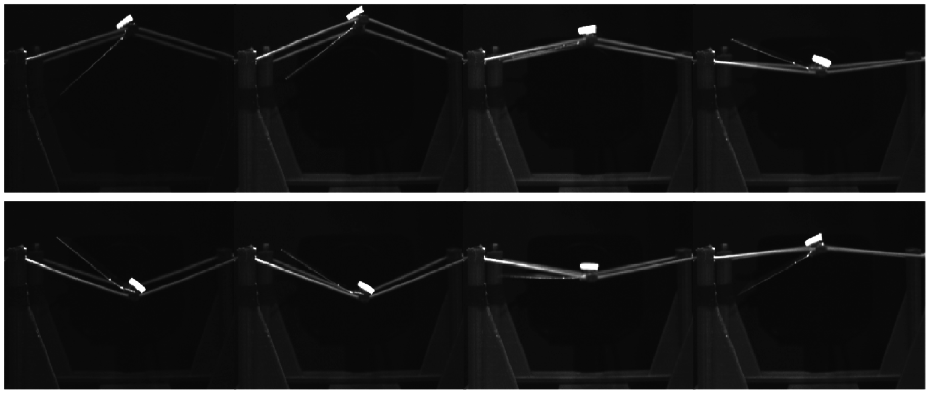
In Figure 2 we report some images extracted from a typical movie. The wind is coming from the right. It is evident that the rigid axis (where the elastomers are fixed) moves along a periodic trajectory in the vertical direction, while the wing oscillates in angle, as Equations (1) and (2) report.

This behavior is due to the aeroelastic interaction of the wind with the system. When the wing assumes a positive angle (counter-clockwise) a lift force is generated, inducing the wing to move up. When the elastic force counterbalances this lift force, the wing rotates around the axis, the angle becomes negative, then reverts to the direction of the lift force. Computational fluid dynamics (CFD) simulations and smoke fluid visualization (not reported here) show that a vortex is created at the leading edge (LE) when the wing reaches an angle (positive or negative) larger than 30°.

These vortices are responsible of the instability that triggers the wing movement, inducing the transition to a stable LCO.

Many parameters influence the shape of LCO: mass and shape of the wing, elastomer strength, and position of the rigid axis along the wing side. Acting on these parameters, it is possible to tune the system in order to maximize LCO amplitude and frequency in a particular wind range.

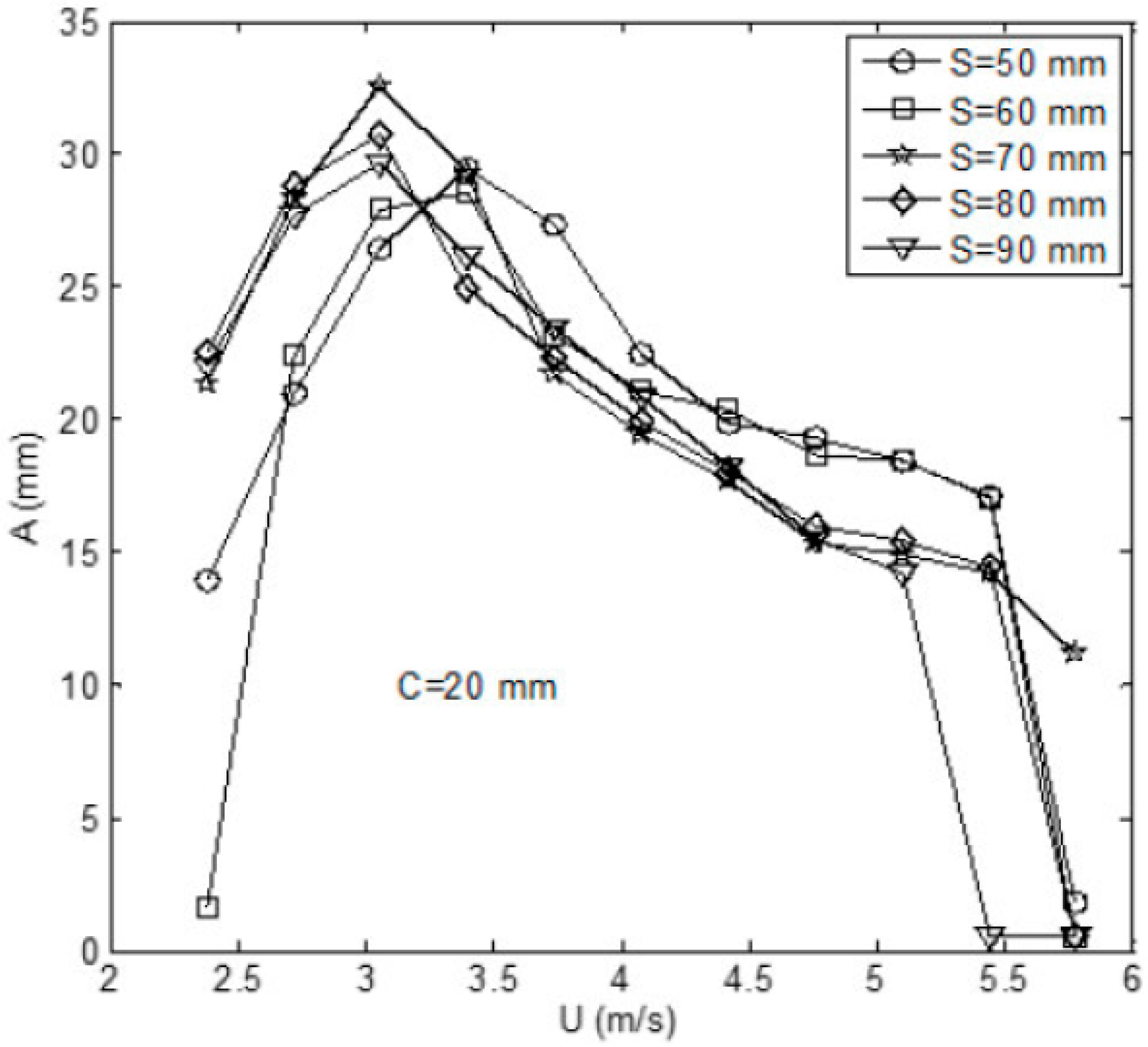
As an example, we show in Figure 3 the LCO amplitude vs. U for a wing with chord = 20 mm and span in the range of 50–90 mm. The system oscillates if the wind velocity is in the range of 2–6 m/s, reaching a maximum at 3 m/s. About the wing angle, it is around 50° (in absolute value) at low velocity, reaches a maximum around 90° at a velocity of 3.5 m/s, then decreases at higher velocities.

For U > 6 m/s, the movement stops and the wing assumes a horizontal position.

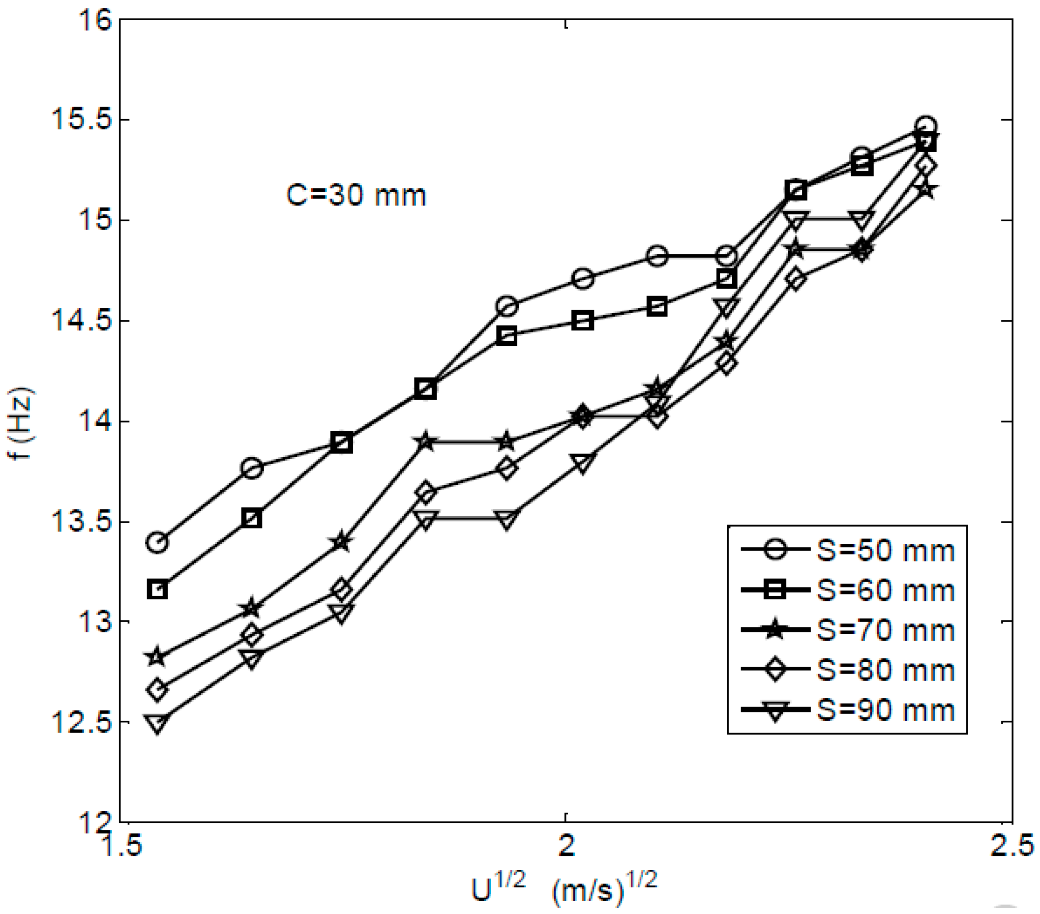
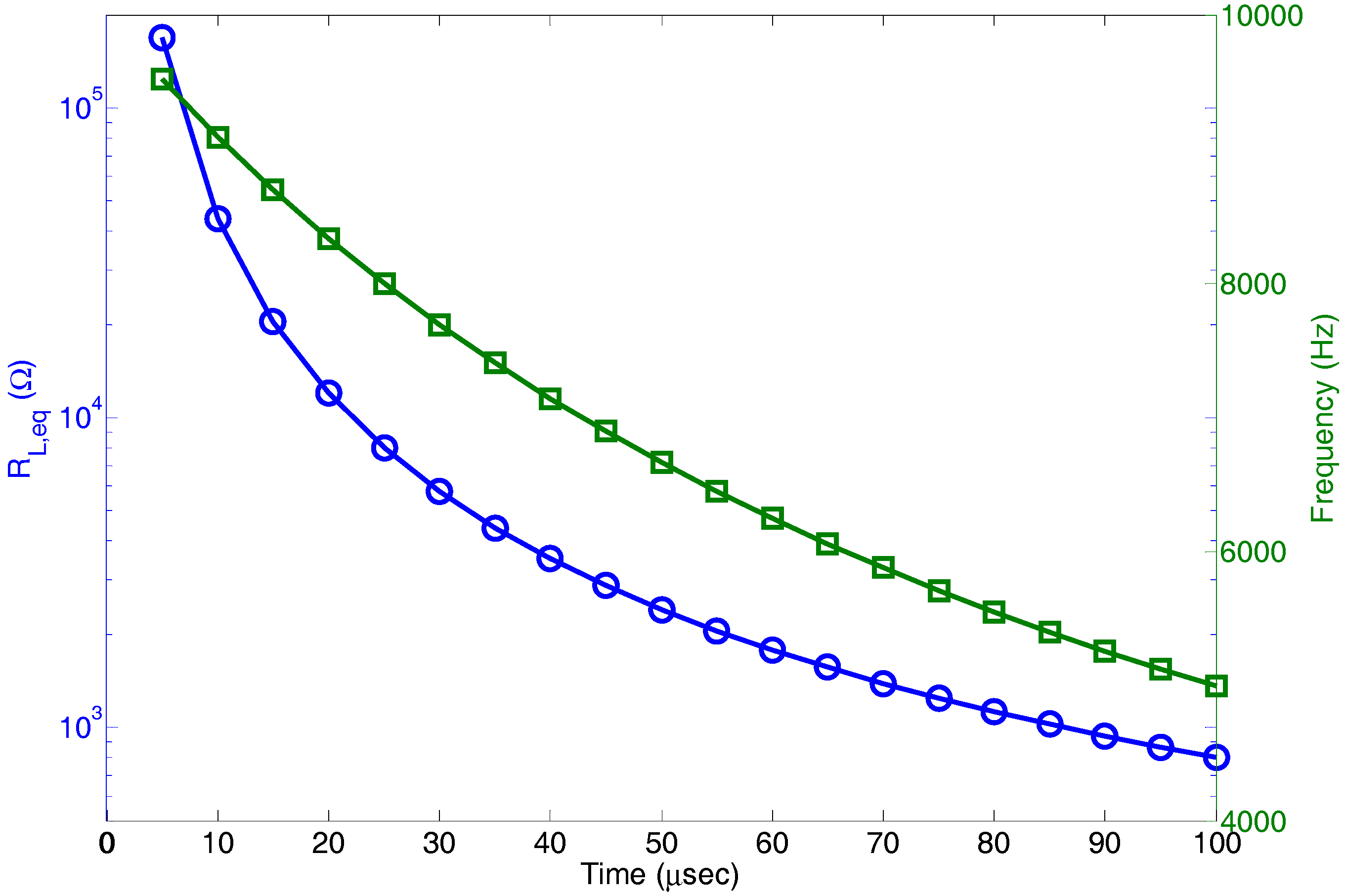
In order to efficiently extract energy from such a system with an electromagnetic coupling, the oscillation frequency needs to be maximized. The measured frequency f is always larger than the natural frequency f_n of the system:

$$f_n=\sqrt{K_{ef{f}_y}/m}$$

(3)

where $K_{ef{f}_y}$ is the effective elastomer strength along the vertical direction and m is the system translational mass.

Frequency f grows with the wind velocity as U^1/2, as shown in Figure 4. We notice that because of this relationship, the FLEHAP device can be used as an autonomous sensor to measure wind velocity.

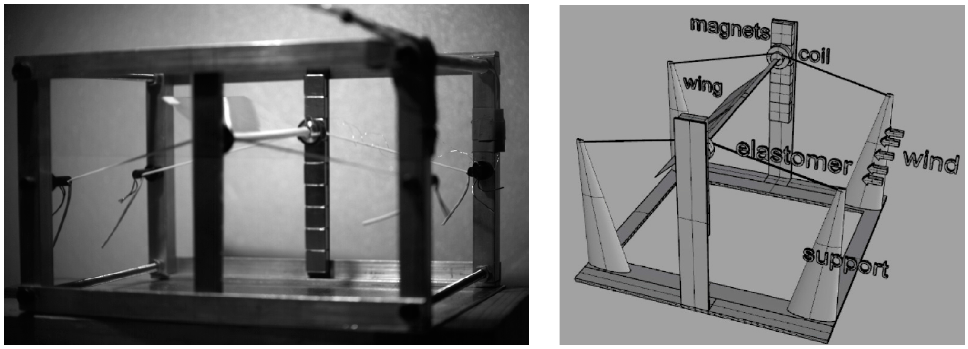
In order to harvest energy from the wing fluttering, the part transforming the mechanical energy into electrical energy uses an electromagnetic coupling: two series of magnets are placed in front of the coils that are fixed at the ends of the rigid axis (Figure 1).

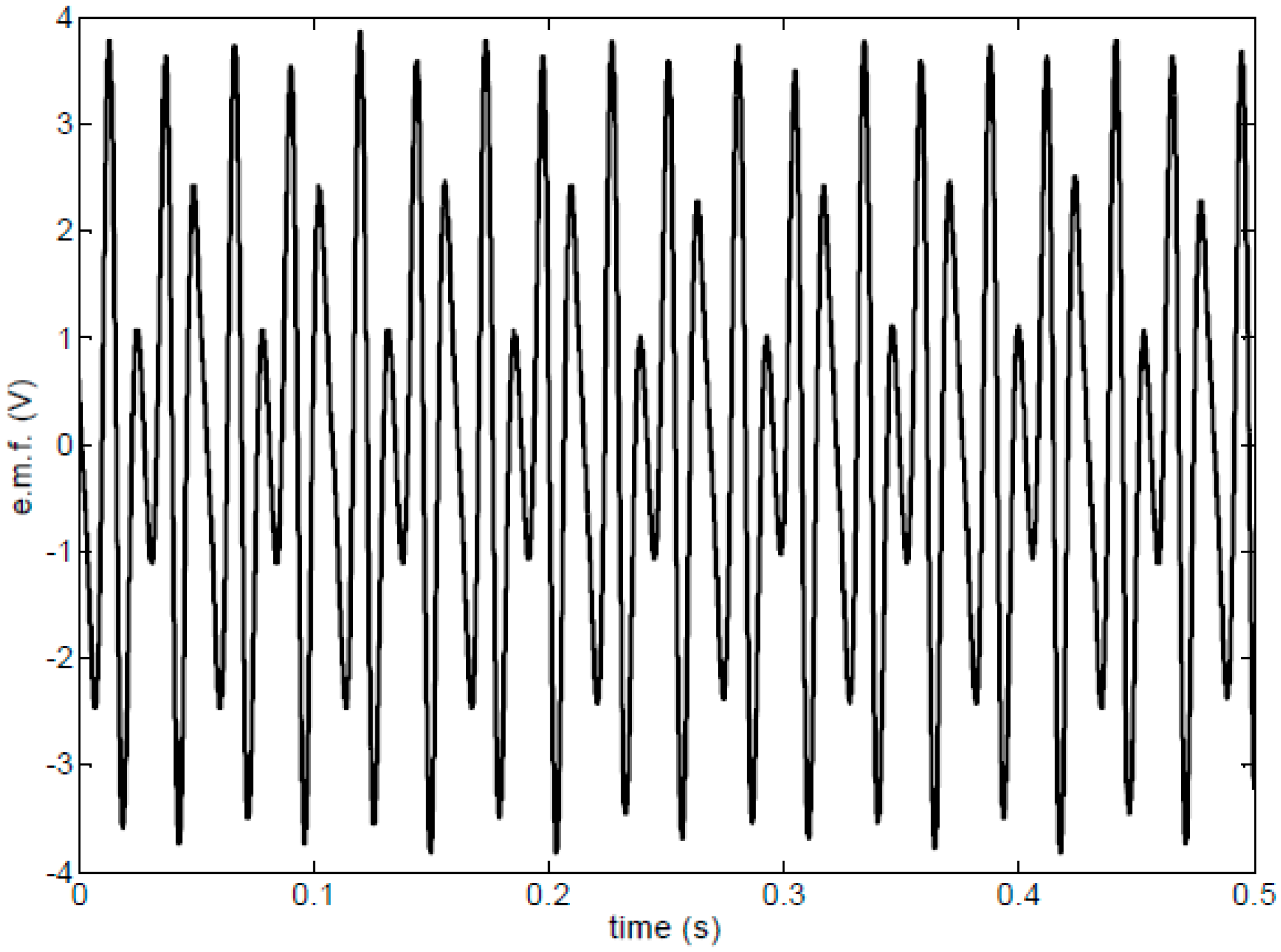
The magnets (NdFeB) have dimensions 10 mm × 10 mm × 4 mm, a coercive field of 38 Moe, and are arranged with alternating polarity N–S–N–S–N face to the coils. The coils have L = 10 mH, R = 150 Ω, 1500 turns, and external diameter 10 mm.

A typical e.m.f. measured during the wing oscillation is reported in Figure 5.

The first evaluation of the FLEHAP device as an energy harvester has been done by simply connecting the coils to a resistive load R_L. Under the wind’s action, the induced current acts as an electromagnetic brake, lowering the frequency oscillation and eventually stopping the wing movement (if R_L is low enough and the wind velocity is not high). Of course, this effect also depends on the other parameters of the system, since the equations describing the system are coupled and nonlinear. A similar effect is discussed in [11]. Then, it is necessary to tune the resistive load for a fixed wind velocity or to choose an R_L value as a compromise that is useful for a larger wind velocity range.

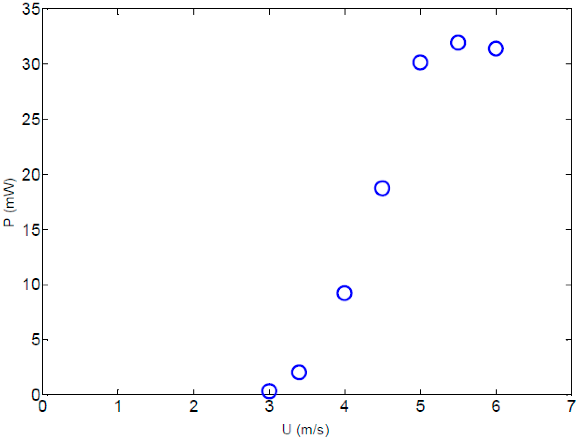
Optimizing the R_L value for each velocity, we obtain the curve reported in Figure 6: in this case, the device starts to produce electrical energy in wind at 3 m/s and reaches a maximum of 32 mW in wind at 5.5 m/s.

Coherent with previous literature studies [12], the efficiency of the device is calculated as the ratio of output electrical power and input wind power, estimated as

$$p_{in}=0.5 \rho A_s{U}^3.$$

With the present device, the efficiency can reach a value greater than 8%.

2.2. Energy-Harvesting Circuit

To efficiently transform the energy harvested by a device into electrical energy, a specialized electronic circuit must be designed. Such a circuit must be adapted to the specific characteristics of the device, and many different solutions have been proposed in the literature [15].

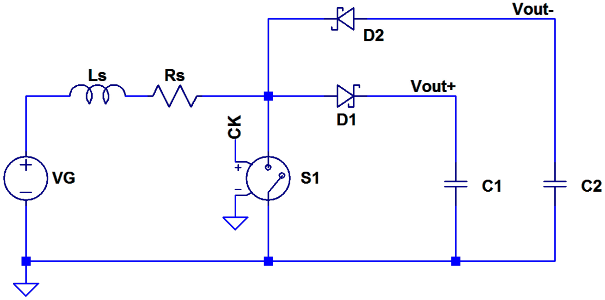
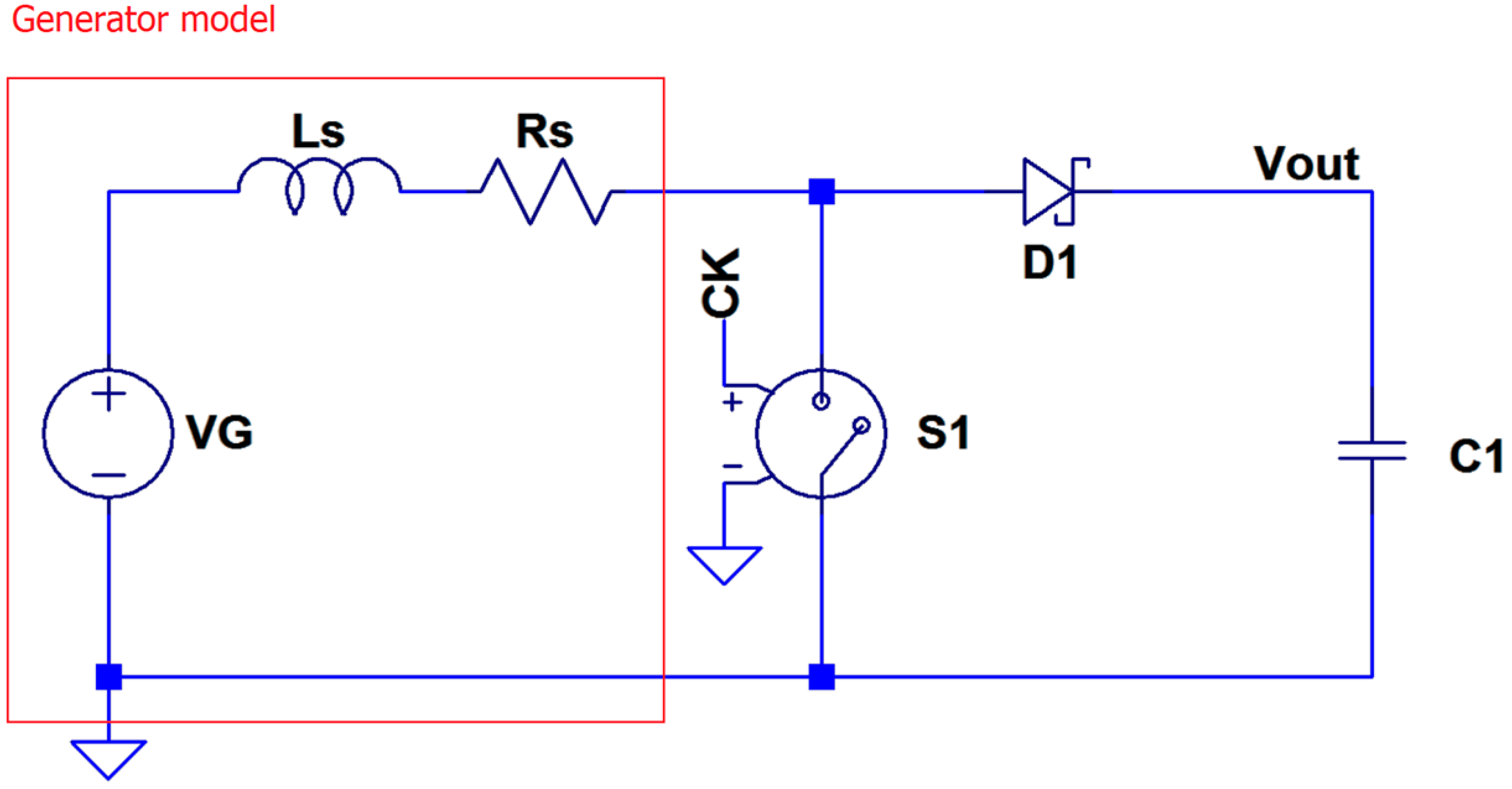
In our case, since we want to possibly obtain a voltage on the supercap higher than the peak value of the input, we chose a boost configuration [15,16,17] that, in its simplest form, consists of a switched inductor converter, as depicted in Figure 7. The red box on the left of the schematics contains the series V_G, R_S, and L_S, which represents the electromagnetic generator obtained as the series wiring of the two coils described previously.

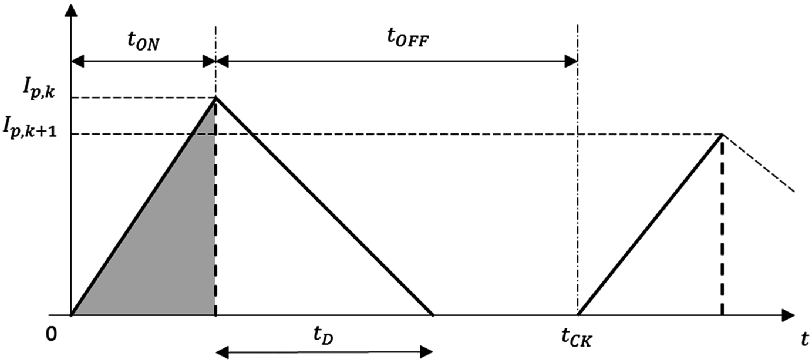
Switch S1 is controlled by a clock signal, CK, with period $t_{CK}=t_{ON}+t_{OFF}$, where $t_{ON}$ is the time interval during which the switch is closed, and $t_{OFF}$ is the time interval it is open (Figure 8). The frequency of the clock signal is $f_{CK}=1/t_{CK}$. We can also define a duty cycle, $D=t_{ON}/t_{CK}$.

Considering the inductive behavior of the generator coils, represented by the inductance $L_S$ and resistance $R_S$ in Figure 7, we can derive a model of the circuit, as seen by the generator, as an equivalent resistive load $R_{L,eq}$. To this purpose, it is worth noting that, considering an ideal switch S1 with a zero value series resistance in the closed state, and a constant input voltage $V_G$, the transient of the current flowing in the circuit follows an exponential behavior as the S1 closes, with a time constant ${\tau }_S=L_S/R_S$ and an asymptotic value ${\tilde{I}}_S=V_G/R_S$. Approaching such a value, most of the power is dissipated on $R_S$. Since what we want is to efficiently extract power from the generator to supply the sensor network node circuitry, we need to reduce the power dissipation on $R_S$ as much as possible, while keeping the possibility of controlling the electromagnetic brake effect on the wing motion.

This can be done keeping the current regime at much values lower than ${\tilde{I}}_S$, which corresponds to adopt a sampling time ${\tau }_{ON}<{\tau }_S$.

For our discussion, let us now relax the constant input voltage condition: as soon as the switch opens, the current starts flowing through the diode and capacitor series. Let us also consider a case in which the capacitor is already charged at a voltage $V_{OUT}$, greater than the sum of $V_G$ and the drops across $R_S$ and the diode.

With these assumptions, we can consider a linear increment of the current as the switch is closed, followed by a linear decrease of duration $t_D$, as represented in Figure 8. It will be a design issue to keep $t_{OFF}\ge t_D$ in all conditions.

Neglecting the voltage drops across both $R_S$ and the switch, we can derive the current value integrating the input voltage:

$$I\left(t_{ON}\right)=\frac{1}{L}{\int }_0^{t_{ON}}{V}_G\left(\tau \right)d\tau .$$

(4)

To compute the equivalent resistance model of the switched inductance, consider first, as a reference, an input signal of arbitrary waveform $V_G\left(t\right)$ loaded with an ideal resistor $R_L$.

In that case, the average power dissipated on $R_L$ over the period $T$ is

$$P_{avg,R_L}=\frac{1}{T}{\int }_0^{T}P\left(\tau \right)d\tau =\frac{1}{T}{\int }_0^T\frac{V_G{\left(\tau \right)}^2}{R_L}d\tau =\frac{1}{R_{L}T}{\int }_0^T{V}_G{\left(\tau \right)}^{2}d\tau .$$

(5)

To carry out the comparison with the switched inductance circuit of Figure 7, let the number of clock cycles comprised in a period of the input signal be an integer number N: $T=N·t_{CK}$.

In this perspective, in the case of large N (e.g., N > 100), it is possible to approximate the input signal, with an acceptable low error, considering its discrete time equivalent $V_{G,k}$ = $V_G\left(k{t}_{CK}\right)$ with $k\in \left[0,N-1\right]$. This expression corresponds to a sampling occurring at the beginning of each clock cycle: different choices (e.g., sampling at the middle of the interval) would not affect our conclusions.

Following this approach, we can write the approximate expression of the average power ${\widehat{P}}_{avg,R_L}$, adapting Equation (3) to the sampled case:

$${\widehat{P}}_{avg,R_L}=\frac{1}{R_{L}T}{\sum }_{k=0}^N\left[{\left(V_{G,k}\right)}^2·t_C\right]=\frac{t_C}{R_{L}T}{\sum }_{k=0}^N{\left(V_{G,k}\right)}^2.$$

(6)

To make a comprehensive comparison of the continuous and sampled case, it is necessary to adapt the latter to manage both signs of the input signal. This can be accomplished via a complementary rectifier as depicted in Figure 9. Positive voltages at the input will produce a charge increment in C1, while negative values will charge C2.

Considering a generic sample k, we can obtain

$$I_{p,k}=\frac{1}{L_S}{\int }_{k{t}_C}^{k{t}_C+t_{ON}}{V}_G\left(\tau \right)d\tau \cong \frac{1}{L_S}{\int }_{k{t}_C}^{k{t}_C+t_{ON}}{V}_{G,k}d\tau =\frac{V_{G,k}}{L_S}·t_{ON}.$$

(7)

The energy available in the inductance for each clock cycle is:

$$E_{L,k}=\frac{1}{2}{L}_S{\left(\frac{V_{G,k}}{L_S}·t_{ON}\right)}^2=\frac{{\left(V_{G,k}·t_{ON}\right)}^2}{2L_S}.$$

(8)

Such energy is transferred to the capacitors during the $t_D$ interval:

$$t_D=\frac{I_{p,k}{L}_S}{V_{OUT,k}+V_{R_S}+V_D-V_{G,k}}.$$

(9)

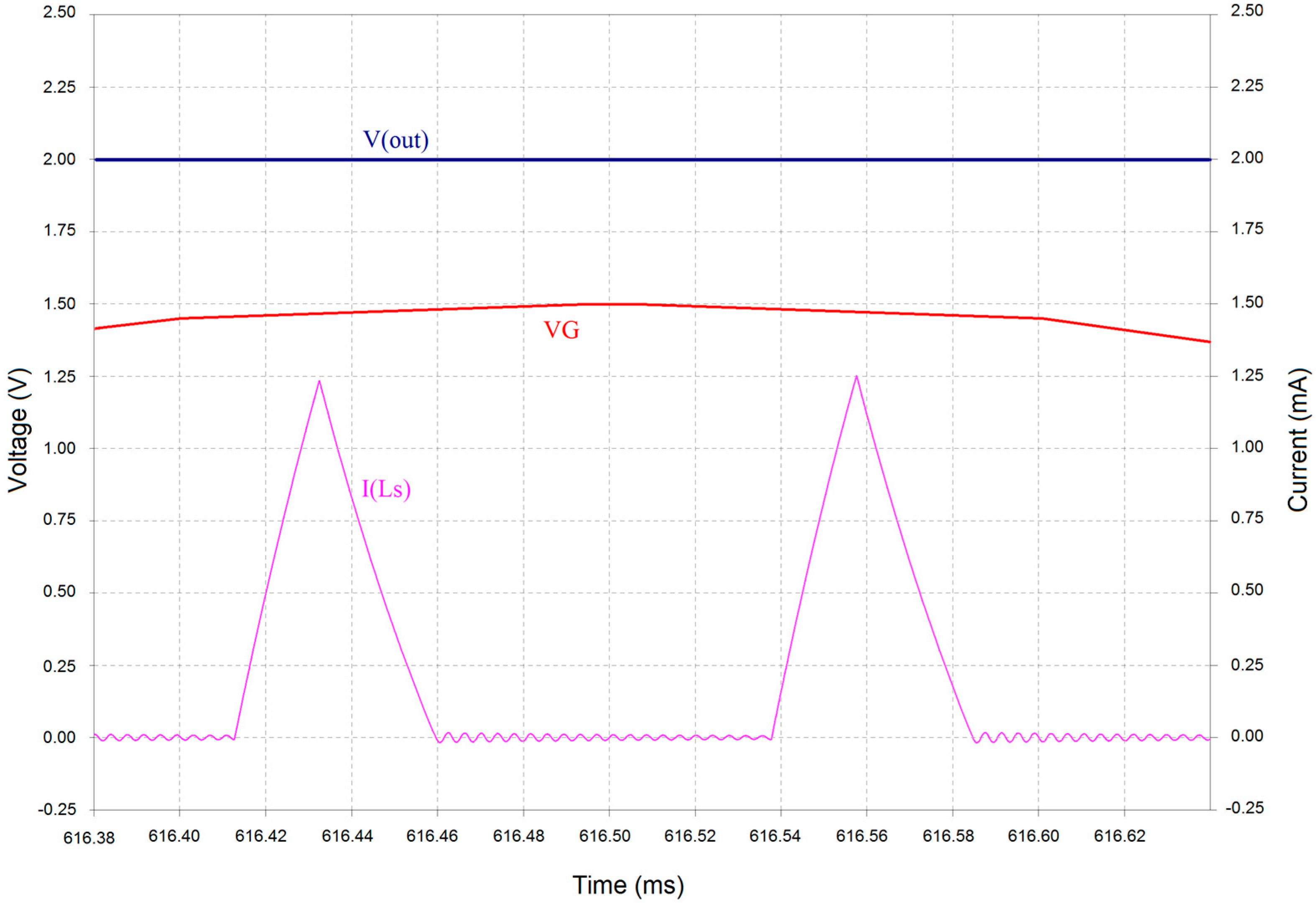
As an example, with $L_S=20 \mathrm{mH}$, $R_S=300 \mathsf{\Omega }, V_{G,k}=1.4 \mathrm{V}, V_{OUT,k}=2 \mathrm{V},$ with $t_{ON}=20 \mathsf{\mu }\mathrm{s}$, the peak current becomes $I_{p,k}=1.1 \mathrm{mA}$. Considering an average voltage drop across the diode of $300\mathrm{mV}$ (e.g., in the case of a BAT54 low-cost Schottky barrier diode), it follows that $t_D\approx 24 \mathsf{\mu }\mathrm{s}$. This is confirmed by the simulation reported in Figure 10. Better results could be achieved using active rectifiers instead of diodes.

Being the original circuit able to manage both signs of the input signal, we can consider that the energy transferred during a period T of the source is:

$$E_T={\sum }_{k=0}^N\frac{{\left(V_{G,k}·t_{ON}\right)}^2}{2L_S}=\frac{1}{2L_S}{\sum }_{k=0}^N{\left(V_{G,k}·t_{ON}\right)}^2=\frac{t_{ON}^2}{2L_S}{\sum }_{k=0}^N{\left(V_{G,k}\right)}^2.$$

(10)

From this equation, we can write the average power obtainable in a period as:

$$P_{avg}=\frac{E_T}{T}=\frac{t_{ON}^2}{2L_{S}T}{\sum }_{k=0}^N{\left(V_{G,k}\right)}^2.$$

(11)

Comparing Equations (3) and (9), and defining $R_{L,eq}$ as the equivalent value to obtain the same amount of energy transfer in the two cases, we can write

$$\frac{t_{ON}^2}{2L_{S}T}{\sum }_{k=0}^N{\left(V_{G,k}\right)}^2=\frac{t_{CK}}{R_{L,eq}T}{\sum }_{k=0}^N{\left(V_{G,k}\right)}^2,$$

(12)

and consequently:

$$R_{L,eq}=\frac{2L_S{t}_{CK}}{{t_{ON}}^2}=\frac{2L_S}{f_{CK}{t_{ON}}^2}=\frac{2L_S}{D^2{t}_{CK}}.$$

(13)

This expression is plotted in Figure 10. This model can be used to optimize the equivalent load and its electromagnetic brake effect to obtain the maximum power transfer.

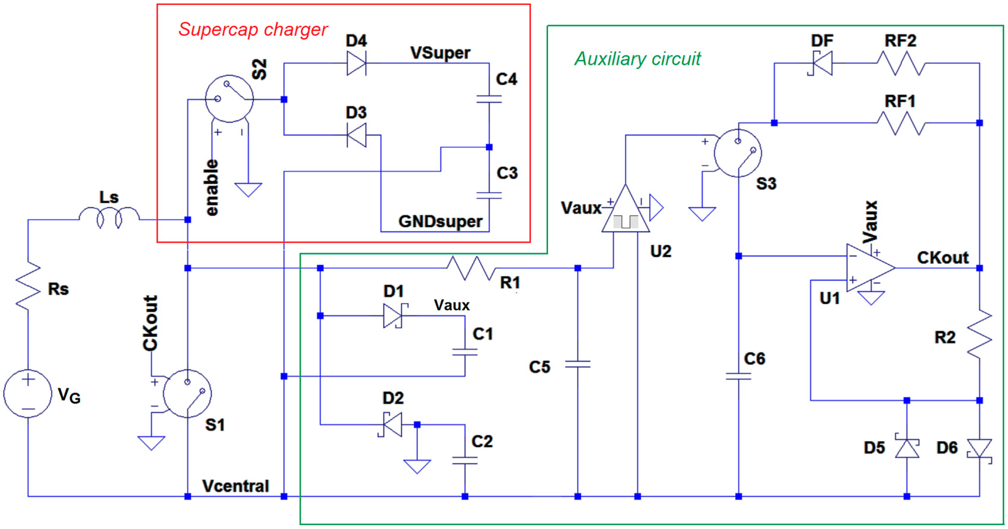
On the basis of such consideration we designed the final circuit shown in Figure 11.

It is worth noting that the circuit has been used for extensive circuital simulation with LTSpice IV [18], modeling the input signal with a simplified piecewise linear generator.

Such circuits consist of two blocks: an auxiliary circuit, and the main rectifier circuit for supercap charging. Both are equipped with a peak-to-peak rectifier (respectively equipped with low-drop diodes D1 and D2 for the first one, and low-leakage diodes D3 and D4 for the latter), for the purpose of maximizing the output voltage available for the user, also in the case of slow wind condition.

The purpose of the auxiliary circuit is to quickly provide power for controlling switches, as soon as it becomes available from the environment. It consists of: (1) an oscillator circuit which generates a clock signal as soon as the $V_{aux}$ voltage reaches the 1.5 V level necessary to bias the comparator U1; and (2) a window comparator (U2) to detect time intervals with no power coming from the generator. The respective functions are:

S1

the main switch is used to clamp the inductor current in the time interval during which the oscillator output CKout is at high level.

S2

when sufficient energy has been stored in the auxiliary capacitors C1 and C2, this switch is turned on to allow supercap charging.

S3

it stops the oscillation when no power is available, to save as much as possible the auxiliary charge stored in C1 and C2.

The circuit has been designed to operate according to the following algorithm:

Starting from a completely zero voltage situation, as soon as some power comes from the generator, the auxiliary rectifier starts charging C1 and C2. As soon as the voltage $V_{aux}$ reaches about 1.5 V, S3 being closed by the window comparator, the oscillator starts working, clamping the intrinsic source inductance Ls.

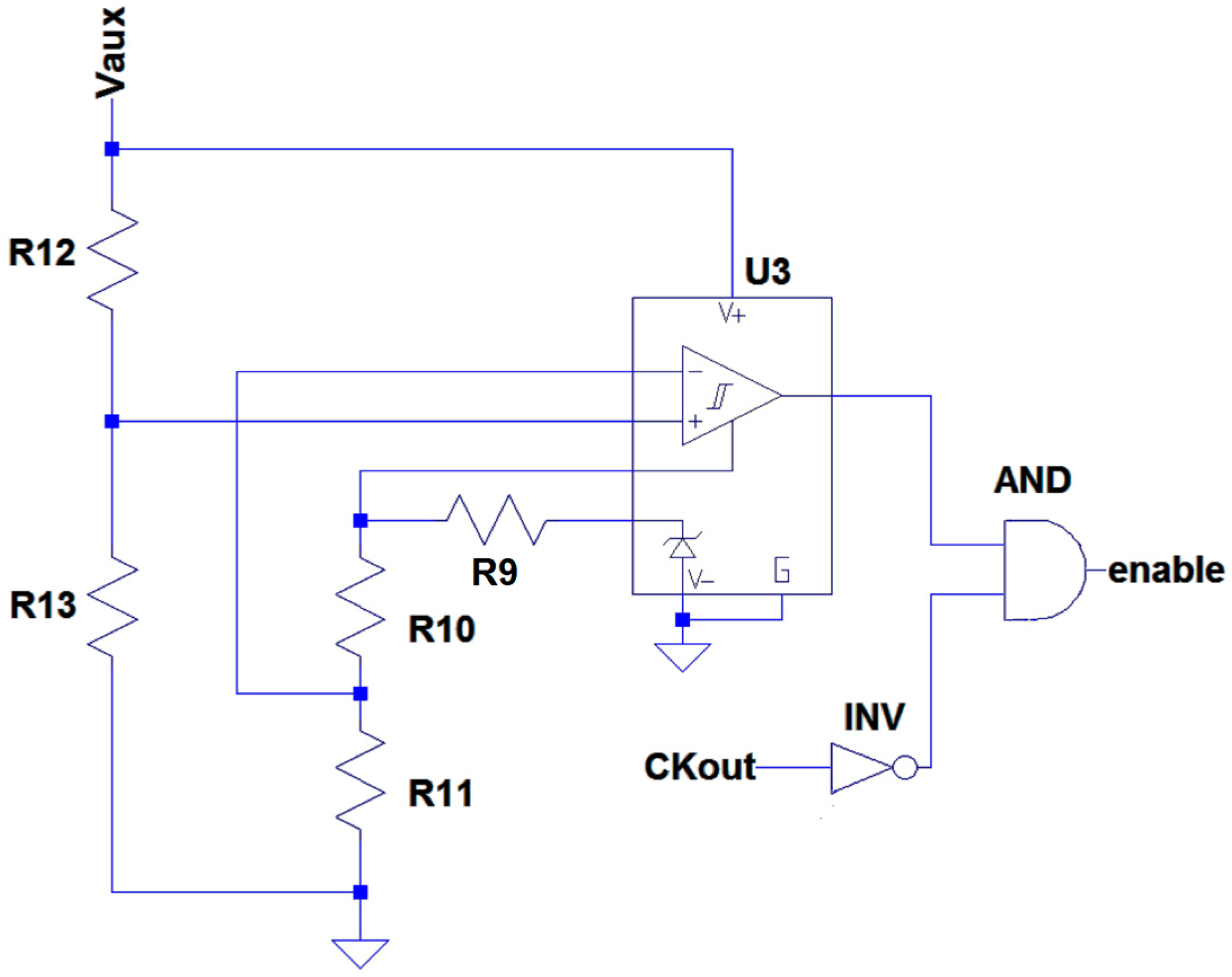
The U3-based Schmidt trigger shown in Figure 12 monitors the $V_{aux}$ level: the auxiliary charging phase continues since an upper limit $V_{a,\max }$ is reached. As soon as this occurs, the S2 switch is enabled, and consequently, the supercap charging phase starts. Since, at least at the beginning, the supercap voltage is lower than $V_{aux}$, the D1 and D2 diodes do not conduct any longer, and C1 and C2 capacitors start discharging. This continues since a lower limit $V_{a,\min }$ is reached on $V_{aux}$: at that threshold, U3 disconnects the supercap leaving C1 and C2 to charge again. Resistances R9–R13 (see Figure 12) define $V_{a,\min }$ and $V_{a,\max }$.

This cycle repeats until the maximum voltage of 10 V is reached on both branches. A Zener diode (not shown) is used to protect active circuits.

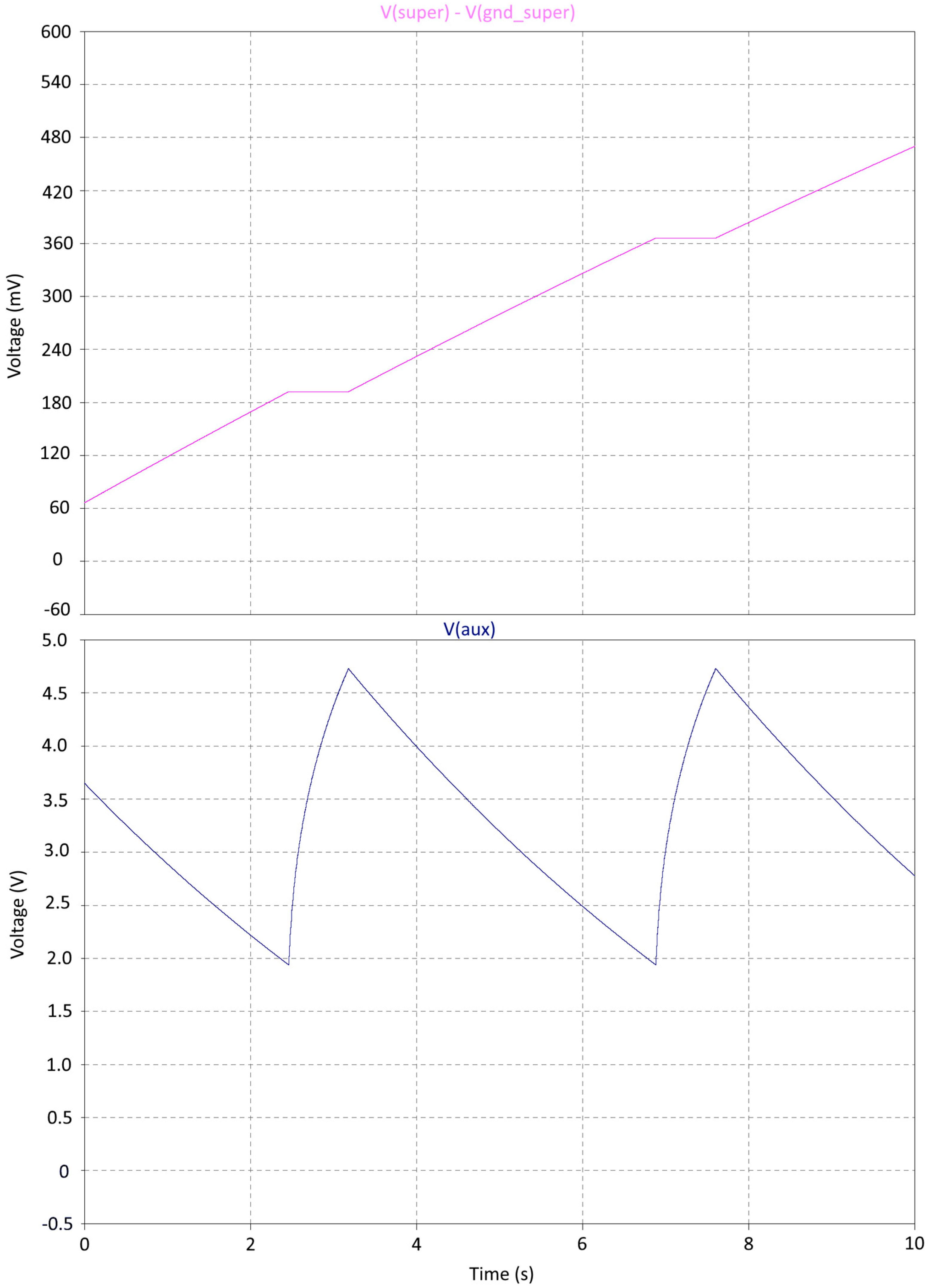
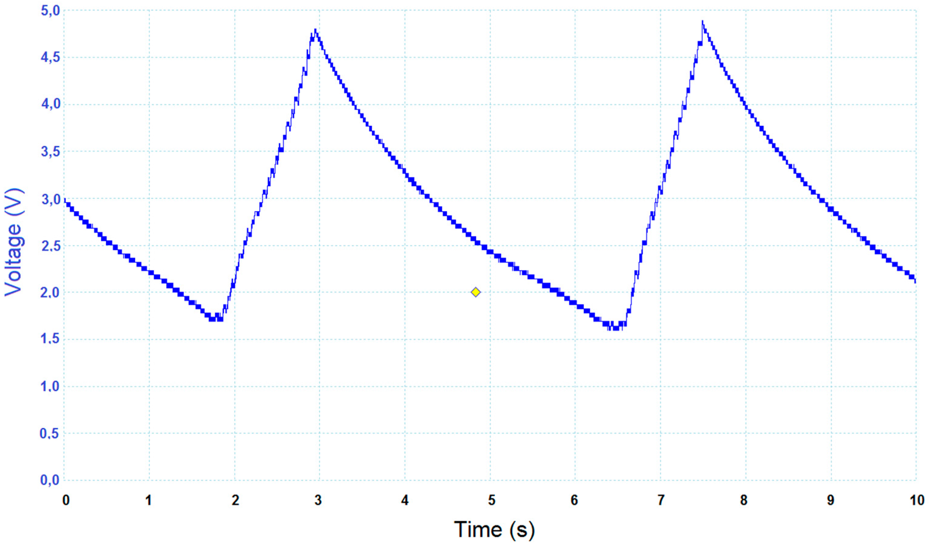
The result of a circuit simulation is show in Figure 13, for a time interval of 10 s. In the example, the following thresholds have been used: $V_{a,\min }=2 \mathrm{V}$; $V_{a,\max }=4.7 \mathrm{V}$. The bottom trace represents the behavior of the auxiliary supply voltage $V_{aux}$, while the upper trace represents the supercap voltage, illustrating the sequence described above. The LTC1540 ultralow power comparator [19] from Linear Technology has been used as U1 and U3, while U2 has been implemented with two open drain comparators contained in a TLV3402 chip from Texas Instruments [20].

The same experiment of Figure 14 has been replicated in the real case with a wind speed of 3.5 m/s, as depicted in Figure 15. When the switch S2 is closed, the $V_{aux}$ signal decreases.

The correspondence with the simulated case reported so far is encouraging.

At the moment, the overall efficiency of the circuit is limited to around 60%: this value is due to the component used and to the correct tuning of the dynamic resistance seen by the generator, which changes with the wind speed. A new version of the circuit is currently under construction.

3. Conclusions

We presented a new energy-harvesting device based on the aeroelastic interaction between a fluid in motion and an elastic structure in which, thanks to the peculiar mechanical configuration adopted, a totally passive pitch and plunge fluttering wing allows it to extract electrical energy from the incoming flow, produced via an electromagnetic coupling between a moving coil and a series of fixed magnets. The experimental results show that the efficiency of this system in centimeter-dimensions-scale is competitive with respect other traditional technologies (e.g., C = 20 cm, S = 70 cm, A_spanned = 50 cm², η > 8%, Re = 4500), such as microturbines [21] and fluttering devices of comparable dimensions on the market [14].

The possibility to easily tune the system by a correct prestretching of elastomers allows extension of the work conditions of the same device; furthermore, the system can be used more simply as a flow-speed sensor.

A specialized electronic circuit has been designed and tested to efficiently transfer the electrical energy to a supercapacitor, demonstrating the feasibility of harvest energy with a switched inductor converter circuit.

The preliminary circuit presented in this paper reach an electrical efficiency conversion of about 60%, and it will be improved with respect considerations of electromechanical performance of FLEHAP.