
An SVM-Based Method for Classification of External Interference in Industrial Wireless Sensor and Actuator Networks


Department of Information Systems and Technology, Mid Sweden University, 851 70 Sundsvall, Sweden
*
Author to whom correspondence should be addressed.
J. Sens. Actuator Netw. 2017, 6(2), 9; https://doi.org/10.3390/jsan6020009
Submission received: 30 April 2017
/
Revised: 3 June 2017
/
Accepted: 12 June 2017
/
Published: 16 June 2017
(This article belongs to the Special Issue QoS in Wireless Sensor/Actuator Networks and Systems)
Abstract
:In recent years, the adoption of industrial wireless sensor and actuator networks (IWSANs) has greatly increased. However, the time-critical performance of IWSANs is considerably affected by external sources of interference. In particular, when an IEEE 802.11 network is coexisting in the same environment, a significant drop in communication reliability is observed. This, in turn, represents one of the main challenges for a wide-scale adoption of IWSAN. Interference classification through spectrum sensing is a possible step towards interference mitigation, but the long sampling window required by many of the approaches in the literature undermines their run-time applicability in time-slotted channel hopping (TSCH)-based IWSAN. Aiming at minimizing both the sensing time and the memory footprint of the collected samples, a centralized interference classifier based on support vector machines (SVMs) is introduced in this article. The proposed mechanism, tested with sample traces collected in industrial scenarios, enables the classification of interference from IEEE 802.11 networks and microwave ovens, while ensuring high classification accuracy with a sensing duration below 300 ms. In addition, the obtained results show that the fast classification together with a contained sampling frequency ensure the suitability of the method for TSCH-based IWSAN.
1. Introduction
The use of wireless sensor networks (WSNs) is a growing trend in a myriad of application domains, including building-health monitoring [1], military applications [2], health monitoring systems [3] and disaster and emergency management [4], to mention a few. A common denominator for many of these networks is the underlying radio technology, which is based on the IEEE 802.15.4 standard [5]. However, depending on the application, different requirements are set regarding the quality of service (QoS). In particular, differently from common implementations of WSN, the requirements found in those deployed in industrial settings, also known as industrial wireless and actuator networks (IWSANs), are considerably more challenging. Furthermore, the inclusion of actuators allows the IWSAN to cover more specific applications, such as closed-loop control, in which bi-directional data-traffic is needed.
IWSANs are characterized by having star or few hops mesh topology with a small number of devices and for presenting stringent requirements on the end-to-end communication delay and reliability. These requirements commonly include downlink and uplink transmission of process data with refresh rates in the order of tens of milliseconds and a network uptime greater than 99.999%, which corresponds to a downtime of less than 5.26 min per year [6]. Fulfilling such communication requirements is critically important in order to enable the adoption of IWSAN as a replacement of traditional wired implementations, such as Fieldbus-based solutions [7]. A failure to meet the QoS requirements can result in unwanted and costly production halts, corruption of the industrial product or even physical damage to production devices and human harm.
The two main factors that hamper the performance of IWSANs are the harsh radio-propagation conditions of most industrial environments, with pronounced effects of multipath fading and attenuation (MFA), and the interference originated from RF emissions in the 2.4-GHz unlicensed industrial, scientific, and medical (ISM)-band. The combined effect of these phenomena can cause severe degradation of the IWSAN radio links, potentially generating prolonged communication outages in some sectors of the wireless network. The RF interference that affects IEEE 802.15.4-based WSNs is mainly generated by wireless systems sharing the same ISM-band and microwave ovens (MWO), while the RF emissions of other devices (e.g., electric motors or switches) is mainly confined to the sub-GHz region of the spectrum, as shown in [8] and the references therein. Nevertheless, while some industrial plants can employ MWO in their production process (e.g., industrial material drying or food processing [9]), the wireless systems that reside in the 2.4-GHz band are much more frequent. The most widespread technologies that operate in this band are the IEEE 802.11 and IEEE 802.15.1 standards, under the commercial name of Wi-Fi and Bluetooth, respectively. IEEE 802.11-based WLANs are generally acknowledged as the most severe cause of interference for a number of reasons. Primarily, IEEE 802.11 networks are now ubiquitous in both office and production areas due to the widespread diffusion of WiFi-enabled terminals, such as smartphones or laptops. Moreover, in order to achieve full coverage, numerous access points are deployed, which can represent an obstacle for coexistence with IWSANs. Additionally, the IEEE 802.11 standard defines a physical layer (PHY), which enables transmission powers ten-times higher than IEEE 802.15.4 devices and a 5–8-times wider channel bandwidth, as shown in Figure 1. As a result, a coexisting IEEE 802.11 network can cause a packet error rate (PER) up to 70% [10,11,12] for a WSN receiver under the worst-case scenarios, such as prolonged use of overlapping channels, proximity of an IEEE 802.11 access point and sustained utilization rate of the interfering network. While devices implementing the IEEE 802.15.1 standard can also be found in industrial settings, thanks to the limited channel bandwidth and the implemented frequency-hopping scheme, their impact on the performance of IEEE 802.15.4-based networks is limited compared to MWO and IEEE 802.11 interference, as reported in [13]. For this reason, the classification of IEEE 802.15.1 interference is not considered in this paper.
Time-slotted channel-hopping (TSCH) is a well-known technique implemented in IWSAN standards, including WirelessHART [14], ISA100.11a [15] and WIA-PA [16], to mitigate the effects of external interference. Nevertheless, none of these standards employs intelligent methods for classifying the source of interference and adopting ad hoc strategies for interference mitigation. Since the first release of the IEEE 802.15.4 standard in 2003, a consistent number of research works has been carried out addressing interference-awareness in WSN. This matter can be separated into two different, but tightly-related aspects: interference classification and interference mitigation. In the terminology of cognitive-radio systems [17], the secondary-users (i.e., WSN-devices) are required to gain a certain level of spectrum awareness in order to utilize the unused resources opportunistically. A common approach for spectrum sensing methods in the literature is to adopt a relatively high sampling frequency and a sensing-time in the order of seconds, in order to maximize classification accuracy or make inference on the inflicted PER [18]. However, this is not suitable in the context of the time-critical IWSANs, where a long spectrum-sensing time implies slow network reactivity to the variations of the interference-scenario and waste of network resources due to the need for reserving numerous silent timeslots for channel sensing.
In this article, an interference detection and classification method is proposed and analyzed, with particular focus on minimizing the time required for channel sensing and the complexity of feature selection, while ensuring a good level of in-channel detection accuracy. For this purpose, a distributed spectrum sensing strategy and a centralized classification algorithm are employed to generate a space-frequency map of interference-free channels (IFCs). The IFC map is valuable information in the context of interference-aware resource scheduling for interference mitigation. The proposed interference classifier uses a three-step classification strategy, comprising a lightweight feature extraction stage, a set of four support vector machines (SVMs) performing preliminary binary classifications and a final stage composed of a logic decisor. The introduced mechanism is able to discriminate among interference from IEEE 802.11 networks, even when no terminal is associated with the access point, RF leakage from MWO and an IFC. Differently from other methods in the literature, such as [19,20,21,22], the proposed method does not rely on features based on the periodicity of IEEE 802.11 beacons. This fact, in conjunction with the novel classification scheme based on multiple SVMs, helps to ensure good classification performance while requiring an extremely limited sensing time.
The main contributions of this work are as follows:
- This is the first study that employs an SVM classifier to process signal features extracted from received signal strength indicator (RSSI) traces to identify the source of external interference. The proposed method employs four lightweight signal features, designed considering hardware constraints of commercial off-the-shelf (COTS) WSN devices.
- It is shown that, in order to ensure good detection performance, the proposed classifier requires a time window for spectrum sensing consistently below 300 ms, which, to the best knowledge of the authors, places the proposed solution amongst the quickest and most reliable methods reported in the literature.
- The performance of the proposed solution is validated by using an RSSI dataset collected in different industrial environments. Both the controlled and uncontrolled interferences from IEEE 802.11 networks are taken into account.
- The often overlooked influence of device calibration on spectrum sensing-based interference classification is analyzed, showing that the classifier accuracy is subject to the intrinsic hardware variations of the employed devices. However, we show that this factor can be easily corrected by means of a straightforward calibration process.
The remainder of this article is structured as follows. In Section 2, relevant work available in the literature about interference classification and mitigation in WSNs is presented. Section 3 provides a general background of the topic, discussing the various sources of cross-technology interference, with specific interest in the IEEE 802.11 standard. In Section 4, the basic concepts and mathematical formulation for SVMs are explained. In Section 5, a detailed description of the proposed solution is given, highlighting feature selection and the structure of the proposed classifier. In Section 6 and Section 7, the experimental setup and the results from experiments are described. In Section 8, the achieved results are discussed, and lastly, conclusions and final considerations are drawn in Section 9.
2. Related Works
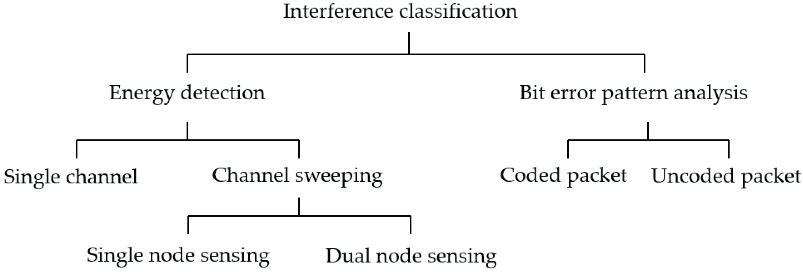
The unrestricted and widespread usage of the unlicensed 2.4-GHz ISM bands, coupled with the asymmetric transmit power and medium access rules, results in harmful mutual interference among coexisting wireless systems. The most affected are the low-power systems, such as IEEE 802.15.4-based WSNs. Various experimental and theoretical studies have highlighted WSNs’ susceptibility to the external interference, especially from high transmit power IEEE 802.11-based WLANs. Many experimental studies (e.g., [10,23,24]) show that an IEEE 802.15.4 link operating on a channel overlapped by an IEEE 802.11 network can experience packet losses of up to 50–70%. In light of these performance studies, it is evident that without an interference detection and avoidance mechanism, WSNs cannot satisfy any reliability or dependability conditions required by the aforementioned industrial applications. The most common interference detection technique, also recommended by the ZigBee standard [25], is to utilize energy detection-based spectrum sensing and avoid the channels with an energy level above a certain threshold. However, in order to design an intelligent interference avoidance technique, the type of interference and its behavior in the time and frequency domains need to be identified first. As interference scenarios may evolve in time, adaptive mitigation approaches with an individual strategy are efficient and are recommended [11]. There exist two main approaches to interference classification, where the distinction is made based on the information source used to extract the features to analyze: (i) raw channel energy measurements (i.e., RSSI samples), and (ii) bit error patterns in a corrupted packet. The existing methods for interference classification available in the literature are shown in Figure 2 and further discussed in the following sections.
2.1. Energy Detection-Based Interference Classification
In this approach, a node actively collects energy samples on one or more IEEE 802.15.4 channels when the WSN devices are not transmitting. Signal processing techniques are then applied to the stored samples in order to extract a number of signal features, according to the implemented method. Hard conditioning or machine learning techniques are then employed in order to map these features to a class of interference, such as IEEE 802.11, Bluetooth and MWO. The advantage of this approach is that no packet transmission is required, since there is no feature extraction from received packets. On the other hand, these methods require a certain time window in order to collect the required energy samples, meaning that specific idle-periods have to be reserved for channel sensing, potentially reducing the availability of network resources for data transmission.
In [19,26], Zacharias et al. propose a lightweight interference classification method in which a series of conditions are tested to identify the dominant source of interference. In these works, a node collects the RSSI samples on a single channel over a duration of one second at a sampling frequency of 8 kHz. The samples are then binarized using a fixed threshold of −85 dBm. Based on the binary data, the temporal features such as channel idle, busy time and signal periodicity are extracted. The classification conditions are then applied to the extracted features to identify the type of interference, achieving a classification time between 600 ms and 700 ms.
The detection of multiple sources of interference is studied by the authors in [27]. In this study, a clustering algorithm is applied to RSSI samples (collected by a node at a sampling frequency of 21 kHz) to distinguish the RSSI bursts from different interferers. In addition, a classifier identifies the channel activity patterns as periodic, bursty or a combination of both to determine channel suitability. The identification of periodic signals such as IEEE 802.11 beacons is also considered, achieving a classification accuracy of over 90% for sampling windows greater than or equal to 3 s.
The detection of the IEEE 802.11 beacons for the discovery of an IEEE 802.11 network has also been the subject of investigation in [20,21,22]. The collection of RSSI measurements over available channel sets (channel sweeping) is considered in [28], which employs two IEEE 802.15.4 radios to achieve pair-wise synchronized channel sensing. The objective of collecting samples over multiple channels is to identify the interference by matching the observed spectral pattern with the stored reference shape. The work targets only IEEE 802.11 interference, achieving a classification rate of 96% with sensing time in the order of 300 ms. In [29], instead, a single node is used for channel sweeping, and an interference classification method targeting IEEE 802.11 and MWOs is proposed in the context of an interferer-aware transmission adaptation mechanism.
Based on the high-resolution scanning feature of Atheros-based WLAN cards, the authors in [30] were able to extract detailed timing and frequency information of the interfering signal, at the cost of using additional hardware. In this context, a decision-tree classifier for interference identification was implemented yielding 91–96% detection accuracy. In [31], Weng et al. have developed two algorithms for the identification of MWO, IEEE 802.11 and Bluetooth signals based on 20 MHz I/Q data sampling performed by means of additional spectrum sensing hardware. However, these approaches are beyond the scope of the hardware capability of commonly-used resource-constrained sensor nodes.
2.2. Bit Error Pattern-Based Interference Classification
This class of methods does not require the active collection of RSSI samples; rather, the interference classification is based on the analysis of bit error patterns in the packets exchanged during the normal operation of the network. In [32,33], the authors show that the different interferers, such as IEEE 802.11, Bluetooth and ZigBee, corrupt IEEE 802.15.4 packets, leaving specific error footprints. In addition, the bit error pattern can also be used to reveal the presence of weak links. In particular, Hermans et al. [32] propose identification of the interference source by combining (i) the signal strength variations during packet reception, (ii) the link quality indicator (LQI) associated with a packet and (iii) the position of corrupted bytes in the payload. The classification accuracy of the proposed method is 72%, while this result is also IEEE 802.15.4 packet size dependent, since packets with a small payload size are partially overlapped with the interferer, thus carrying a small interference fingerprint. In [34] Barac et al. use forward error correction (FEC) in order to identify the source of bit errors in a received packet (i.e., multipath fading and attenuation, as well as the IEEE 802.11 b/g interference). Therefore, instead of packet retransmissions (which is used in [32]), the FEC method in [34] emerges as an energy-efficient alternative for interference classification, yielding more than 91% classification rate with just one received packet.
3. Background
3.1. Cross-Technology Interference Sources
In this section, we discuss the salient features of the cross-technology sources of interference targeted in the current work, namely IEEE 802.11-based WLAN and MWO.
3.1.1. IEEE 802.11
The prevalent WLAN networks in the 2.4-GHz band are based on the IEEE 802.11 b/g/n specifications. The IEEE 802.11 b/g PHY supports up to 14 channels, 20 MHz wide each. On the other hand, the IEEE 802.11 n can support both the 20 MHz- or 40 MHz-wide channels. There are only three non-overlapping usable channels in the U.S. and other countries with similar regulations (Channels 1, 6, 11, with 25-MHz separation) and four in Europe (Channels 1, 5, 9, 13, with 20-MHz separation). The transmit power of WLAN devices ranges from 15 dBm–20 dBm, and depending on the underlying standard, different modulation schemes and data-rates are available. However, the maximum air-time of an IEEE 802.11 packet remains below 600 s. The standard specifies a carrier-sense multiple access with collision-avoidance (CSMA/CA)-based MAC with certain timing rules between the consecutive packets. In commonly-used infrastructure mode, an access point advertises the network by sending the periodic beacon frames. For compatibility reasons and in order to increase the network detection range, the beacons are usually sent at the lowest data rate (1 or 2 Mb/s). The default beacon frequency period is 100 time units, which is equal to 102.4 ms [26]. The above-stated heterogeneous medium access rules and PHY specifications for WLAN networks render ZigBee systems vulnerable. Firstly, WLAN networks deployed on non-overlapping channel allocation, such as the typical configuration, leave a small number of IFCs for ZigBee. Secondly, the high-power concurrent transmission on an overlapping channel from a WLAN device will likely cause severe packet corruption in an IEEE 802.15.4 packet. Thirdly, the duration of an IEEE 802.15.4 clear-channel assessment (CCA) is 128 , while 192 [14] are required to switch from CCA to transmit mode. Conversely, the IEEE 802.11 CCA procedure takes 28 , while the switching time is negligible. As a result, the chances of the corruption of a ZigBee packet are very high, as the WLAN transmission can disrupt the ZigBee transmission during the switching mode.
3.1.2. Microwave Ovens
The energy leakage from the residential MWOs usually affects the whole 2.4-GHz band. However, as depicted by various studies [29,35], the RF emissions from MWOs peak at about a 2.45-GHz frequency, while the number and center frequencies of peaks may vary slightly according to the specific model, as shown in [36]. As a result, the IEEE 802.15.4 Channels 20 and 21 have a high probability of being strongly affected by the MWO operation. A prominent feature of MWO is the periodicity of on and off phases during the heating process, where the time from one on phase to the next is s, with f the frequency of the power supply (i.e., 50/60 Hz).
4. Support Vector Machines
In this section, we outline the basic formulation of the mathematical problem for an SVM, focusing on the training and classification tasks, while we leave more in-depth analysis to specific machine-learning literature, such as [37], and to [38] for details about the related convex optimization methods.
4.1. The Standard Model for SVM
An SVM is a supervised classification algorithm that allows a binary decision to be performed, assigning an M-dimensional feature-vector to one of two classes. Being a supervised approach, an SVM needs to be trained using an appropriate dataset, which should be sufficiently large and representative of the two classes, with respect to the selected features. A training phase is then needed to determine a subset of the training vectors (called support vectors), which will actually be used for solving the classification problem. One important advantage of SVMs resides in the fact that the number of support vectors is generally much smaller than the cardinality of the training dataset. Hence, while the training of the SVM can be a resource-intensive task, the actual classification algorithm can be very slender. The standard formulation for a two-class classification problem is:
which is a linear model where is the M-dimensional input vector, M is the size of the feature space, is the vector of coefficients for the linear model, is a general feature-space transformation function (which can eventually be non-linear) and b represents the bias of the model.
Hence, the training set for the SVM is composed of a set of N training feature-vectors where each vector is associated with one of the two classes via the parameters , which are the class labels for the training vectors. The decision logic is then the following: an unknown vector belongs to class , if and to class if . The implicit assumption is that the training data are linearly separable, so that the coefficient vector and the parameter b can be determined (i.e., there exists at least one feasible combination of and b).
4.2. SVM: Training and Classification
The training of an SVM can be seen geometrically as the problem of maximizing the minimum Euclidean distance between the decision hyperplane and the points of the training set. This problem can be formulated in an equivalent fashion, observing that since are the target values for the two classes, the following is verified for any correctly-labeled input vector :
It can be easily shown that the optimization problem can be expressed as:
with . Hence, due to the definition of two-norm, the function to minimize in (3) is a quadratic cost function with M variables. The optimization problem that arises is then a quadratic program (QP) with M variables (size of the feature space) and N inequality constraints (size of the RSSI input vector).
Once the model is trained, the solution of the decision problem for a generic input vector can be obtained by simply evaluating the sign of in the original linear model , with the coefficient vector populated using the results from the minimization of the cost function in (3), hence calculating:
where are the Lagrange multipliers of the dual problem. Equation (4) is subject to the Karush-Kuhn-Tucker (KKT) conditions:
An important result is that each point of the cost function for which the respective Lagrange multiplier can be discharged, since it will not influence the calculation, yields a consistent reduction of the dataset size, which is one of the key advantages of SVMs.
5. The Proposed Solution
5.1. Classifier Setup
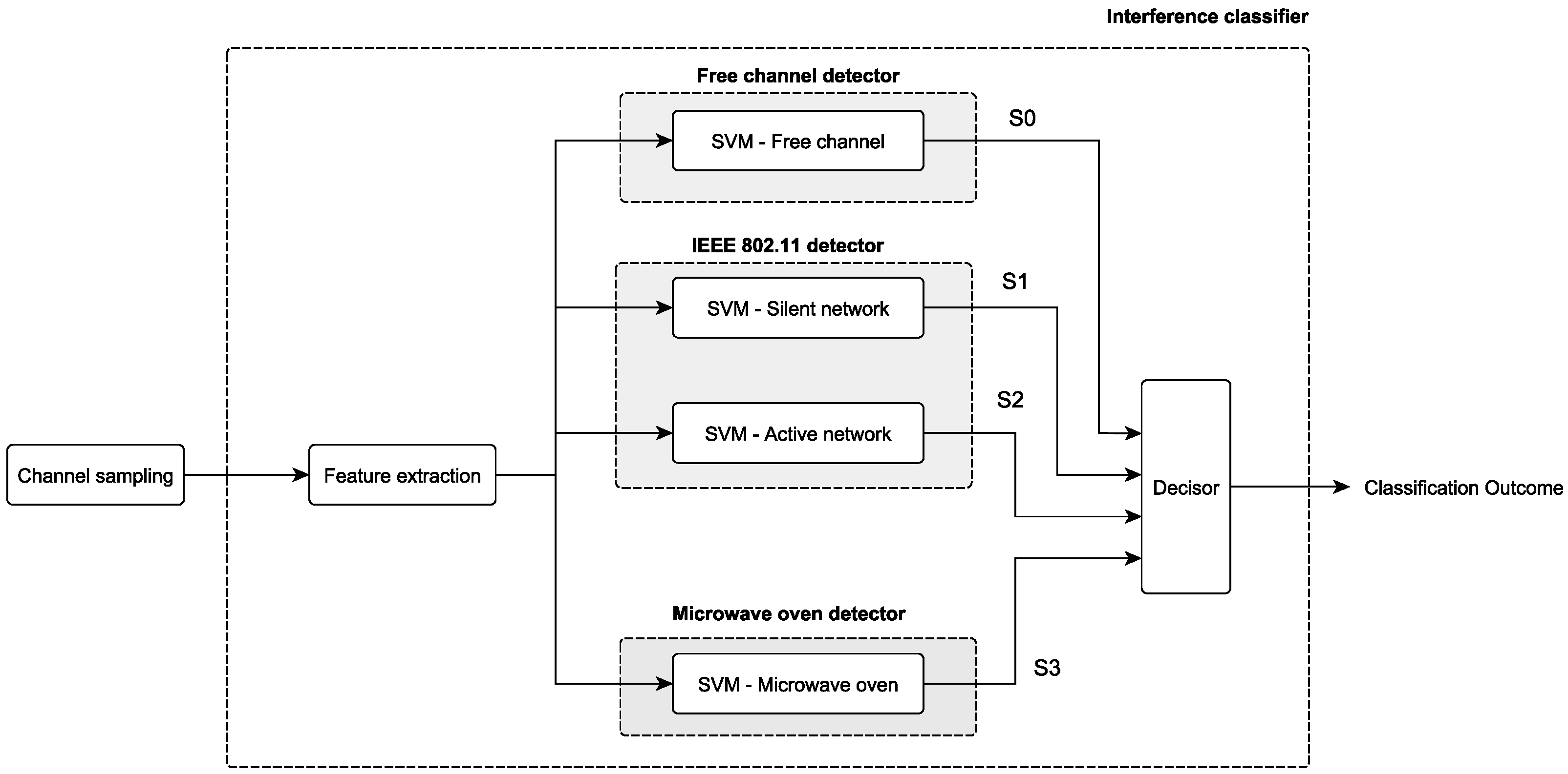
The proposed interference detection method employs an SVM-based classifier, which processes input data composed of observations of the background RF noise on a specific IEEE 802.15.4 radio channel. The method is based on the basic assumption that when there is no transmission on a certain channel (and thus, there is an absence of intra-network interference), the devices can collect samples of the RF radiation and process the data to detect and classify eventual interferers, as well as assessing the eventuality of an IFC. This assumption nicely fits with the time-division multiple-access (TDMA) approach employed in ISWANs, since in these networks, the allocation of frequency-time resources for data transmission is known a priori; thus, a contiguous set of time slots on a specific channel can be reserved for spectrum sensing. The common hypothesis for spectrum sensing is that the classification can be done with a certain level of accuracy if the time window is sufficiently long for specific signal features to emerge. The proposed solution is designed to keep this detection time as short as possible. As shown in Figure 3, the first stage of the classifier employs a process of signal feature extraction, in which data are processed in order to extrapolate a number of signal features in the time and amplitude domains.
The second stage of the classifier is composed of four SVMs, which perform a first decision stage, outputting single binary partial hard decisions with respect to the related interference scenarios. The different SVMs are hereby described:
- SVM-free channel: this SVM is trained to detect the presence of an IFC.
- SVM-active network: targets the presence of an active IEEE 802.11 network occupying the related IEEE 802.15.4 PHY channel (i.e., an IEEE 802.11 access point with at least one associated terminal, generating uplink/downlink traffic).
- SVM-silent network: targets a silent IEEE 802.11 network overlapping the specific channel. This is the case of an IEEE 802.11 access point with no associated terminal or an access point with associated terminals that are not generating data traffic in the observation time window.
- SVM-microwave oven: detects the presence of RF leakage from a microwave-oven operating in close proximity to the radio node.
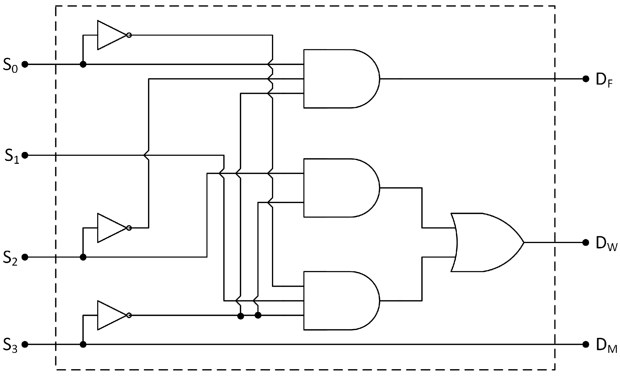
The outputs of the four SVM are represented by binary signals, , , and , which have the value 1 (0) if the related decision is positive (negative). The binary decisions preformed by the SVMs are then processed by the logic decisor shown in Figure 4. The logic function of the decisor has been synthesized considering the cross-detection resilience of the single SVM. The final decision is composed of the four different classes listed in Table 1.
It must be highlighted that the classification performed based on the observation of a single radio node of the network only has local validity. This is because radio devices located in different locations of an industrial plant may be subjected to different interference conditions. In this context, the proposed method allows the interference scenario to be captured for each of the deployed nodes, opening the possibility of mapping the different sources of interference in the space-frequency domain. Nevertheless, since the aforementioned classification scheme exhibits a computational complexity that is beyond the capabilities of COTS WSN nodes, the proposed implementation relies on a centralized classification in place of a distributed approach. This, in turn, means that while the classifier can be implemented in the IWSAN network manager, the spectrum sensing and feature extraction process can be carried out by IWSAN nodes. This approach appears rather convenient, since, as described in Section 5.2, the signal processing required for the extraction of the selected signal features is kept to a minimum, while the efficiency of the classifier allows the radio nodes to work with small RSSI sample traces.
5.2. Signal Features
We select four signal features, belonging to two main classes: time domain and amplitude domain. The logic behind the selection is related to the properties of the interfering signals, such as the transmission airtime of IEEE 802.11 transmission and the periodicity of time domain pattern of the MWO RF leakage, as discussed in Section 3. To simplify the feasibility of the whole spectrum sampling and feature extraction processes on COTS WSN devices, our approach is to minimize the size of the RSSI trace, as well as the complexity of feature calculation methods.
5.2.1. Number and Length of Signal Bursts
The first time domain feature includes information about the burstiness of the observed signal, employing a threshold-based burst detection. The feature is an M-element vector in which each element represents the number of bursts of a certain sample length. Hence, we define:
where represents the the number of bursts of length n found in the RSSI trace in the analysis, while with , we mark all of the bursts with sample length . In particular, we require a certain number of samples under the selected threshold to identify the end of a burst. This is to avoid the case where a single or a few incorrect readings of the RSSI register will lead to a misclassification of long signal bursts into shorter ones. As will be discussed in Section 7, the detection of longer (i.e., > 5 ms) bursts is extremely important because it is a specific feature of the RF emissions of microwave ovens. The choice of a proper value of the threshold with respect to the calibration of the radio nodes will be discussed in Section 6.
5.2.2. Mean, Variance and Cardinality of Over-Threshold Samples
The second feature belongs to the amplitude domain and is defined as the mean value of the RSSI samples over the selected threshold . We define the vector containing all of the RSSI samples collected during the continuous observation window as . Then, indicating with the subset of , such that :
with representing the cardinality of , hence the number of above-threshold samples in the set. The third feature follows directly from the definition of sample variance, hence using the same notation employed for :
The last feature counts the occurrences of RSSI samples above the threshold and hence is simply the cardinality of the set . This feature nicely complements the previous two, adding information about the activity level of the interference source. It must be noted that while the signal features , and are scalars, the feature is an M-element vector; hence the SVM feature-space will be -dimensional, even using only four features.
6. Experimental Setup
6.1. Hardware Setup
The WSN devices selected for the experiments are Crossbow’s TelosB motes CA2400 [39], equipped with Texas Instrument CC2420 transceiver [40]. The devices are programmed to collect a continuous set of RSSI samples with a sampling frequency of 2 kHz, over a sampling window that is selected according to the specific experiment. The RSSI value for each sample is fetched from the first 8 bits of register 0x16 of the CC2420 transceiver and represents the incident RF power in the selected 5 MHz-wide channel averaged over (hence, eight IEEE 802.15.4 O-QPSK symbols). The RSSI data, fetched from the register in the form of an 8-bit signed integer, are buffered in the RAM and periodically saved to the internal flash memory. At the end of the sampling process, the content of the flash memory is sent over the USB port to a laptop, which logs the received data. The choice of this method for collecting RSSI data, in place of the direct sample-and-send over USB approach, was due to the insufficient bitrate (i.e., 115,200 baud including serial message overhead) available at the serial interface. In order to validate the performed measurements, we time stamp all of the observations and measure the delay of the instructions and task implemented in Tiny OS. This aspect will be further discussed in Section 8.2.2. Since Chen et al. [41] reported a consistent offset among RSSI readings performed with CC2420-equipped radio devices, we have also profiled our devices by means of a simple calibration process. We will discuss the effect of node calibration as well as the effect of this process on the performance of the proposed solution in Section 8.2.1.
6.2. Test Environments
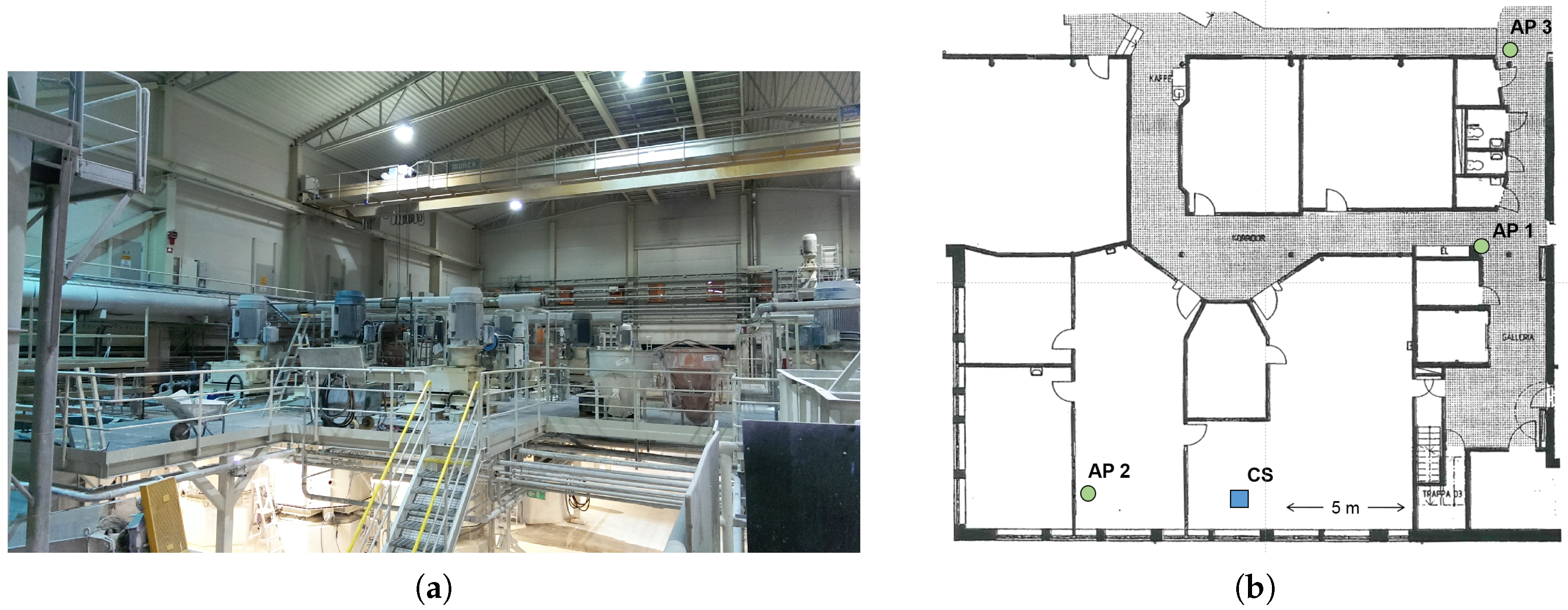
The collection of experimental data has been carried out in three locations. Location A is a three-storey production plant employed for mineral processing. The environment is an open space cluttered with metal tanks, production machinery and a radio-controlled crane, while the three storeys are separated by metal grate flooring. A resident IEEE 802.11 WLAN covering the whole production plant was running at the time of the experiments.
Location B is a small mechanical workshop with an abundance of metal cluttering and soldering tools. A total of fourteen IEEE 802.11 access points with overlapping spectrum allocation on Channels is detectable in this environment. In Figure 5, we show the position of three of the nearest access points, which we label with AP1, AP2 and AP3, while the remaining devices were placed outside the range of the map, or on the upper floors of the building.
Location C is an office area, with nine IEEE 802.11 access points and residential MWO. We use this location to perform experiments on the classification of microwave interference, since neither industrial, nor residential MWO were present in the other two selected sites.
6.3. The Collection of Training Data for SVM
As described in Section 4, the availability of a representative training dataset is fundamental for supervised-learning classification algorithms such as SVMs. Hence, particular attention has been put into building the dataset from both controlled and uncontrolled sources of interference and covering all 16 IEEE 802.15.4 channels.
6.3.1. Training Data from Uncontrolled IEEE 802.11 Networks
A preliminary set of measurements is collected in Location A, by means of Metageek channel analyzer [42], in order to determine the ground truth on the spectrum allocation of the resident IEEE 802.11 access points present at the industrial site. The network was composed of three IEEE 802.11 b/g/n access points statically allocated on IEEE 802.11 Channels 1, 6, and 11.
The training set is collected by means of a TelosB mote deployed in a fixed location of the industrial plant, programmed to sense each IEEE 802.15.4 channel for 10 min, collecting traces with over 1 M-sample per channel. Subsequently, the traces collected from the sampling of IEEE 802.11 Channels were assigned to the IFC class, since the IEEE 802.11 network did not overlap these channels (as shown in Figure 1), while the remaining traces were assigned to class IEEE 802.11 interference.
6.3.2. Training Data from Controlled Sources
The dynamics of an IEEE 802.11 network can vary greatly according to several factors (e.g., the number of connected devices and the traffic data-rate), and this in turn reflects the characteristics of the observed RSSI sample trace. While different methods for generating controlled interference are available in the literature, such as the one presented in [43], we use IEEE 802.11 hardware and a server-client architecture in order to have full control over the traffic distribution and transmission parameters. Following this approach, a controlled IEEE 802.11 network has been deployed at Location A. The structure of the network is represented in Figure 6 and is composed of a Linksys WRT610N IEEE 802.11 access point connected by an Ethernet cable to a Linux laptop running a traffic generator application generating the user datagram protocol (UDP) traffic with uniform, exponential and Pareto distributions. A second laptop, employing a Wi-Fi interface and running a Linux client, was used to receive and monitor the IEEE 802.11 packets. The access point was set on Channel 3, in order to overlap IEEE 802.15.4 Channel 15 (which was not affected by the resident industrial network), in order to isolate the observation from the effects of the resident network and capture only the effects of the custom IEEE 802.11 network.
6.3.3. Training Data from Microwave Oven
A set of measurements was collected in proximity (1 m) of a consumer Samsung MW82Y MWO set at the maximum heating power, achieving an active-passive heating phase with a duty cycle of 50%. The training data were collected along all of the IEEE 802.15.4 channels, since the temporal features of RF emissions from MWO can vary considerably moving within the 2.4-GHz ISM band due to the employed technology, as discussed in Section 3.
6.3.4. Test Data
We collected an extensive test dataset in the three described locations in order to thoroughly test the proposed algorithm.
At Location A, multiple RSSI traces from both the resident IEEE 802.11 network and the access point employed in the experiments were collected over all of the IEEE 802.15.4 channels. The traces were collected at several points of the three floors of the factory, taking care of including both line-of-sight (LOS) and non-line-of-sight NLOS propagation scenarios between the access points and the sensing node.
At Location B, we instead deployed the sensing node at one fixed point of the workshop (Point CS in Figure 5) and sensed each of the 16 channels for 5 min. At Location C, we deployed the radio node in the proximity of the active MWO, taking care of collecting measurements for all of the channels, randomizing the node position in the range 0.5 m–2 m from the oven. In all of the data collection points of the selected locations, the spectrum analyzer was used to determine the actual interference status of the sensed channels (similarly to the training data collection process), in order to determine the ground-truth for assessing the performance of the off-line classifier.
7. Results
7.1. Global Classification Accuracy
We tested the performance of the proposed algorithm by splitting each of the RSSI traces into several data chunks, with a length varying according to the tested sampling window, in the range of 50–500 ms. The data chunks were then processed in MATLAB, where we implemented the proposed classifier, including the feature extraction process and the four SVMs using the standard MATLAB SVM implementation with the Gaussian kernel, as well as the final decisor stage. For each test set, we calculated a detection accuracy metric by analyzing the outcome of the predicted interference source (according to Table 1) and comparing to the actual source determined during experiments. The detection accuracy was then simply calculated by dividing the number of correct classifications by the total number of classification rounds. In Table 2, we show the classification rates calculated for Locations A, B and C, including test data for all 16 IEEE 802.15.4 channels when the sampling widow is 250 ms; hence, chunks of 500 eight-bit RSSI samples are analyzed in each round of the test. It should be noted that the validity of the presented results is expected to be quite broad in nature as our dataset includes extensive traces from a broad range of scenarios including both controlled and uncontrolled IEEE 802.11 interference, spanning all of the IEEE 802.15.4 channels. A more in-depth discussion of the effects of a shorter or longer sampling window on the accuracy of the solution will be carried out in Section 8.1. In the following tables, we also include data about the distribution of misclassification in order to highlight which sources of interference were most likely to be misinterpreted by the classifier.
As shown in Table 2, the classifier was able to determine the presence of a free IEEE 802.15.4 channel of the time, and the primary source of misclassification was the IEEE 802.11 network, which was detected of the time. This fact is mainly due to the similarity of RSSI traces originating from an IEEE 802.11 network with low data traffic or even no associated terminal with RSSI originated from background noise. The similarity becomes more prominent when the signals originating from an IEEE 802.11 network and received by the WSN node are weak, due to attenuation effects. The same effect can also be used to explain the IFC misclassification rate of when the interference comes from an IEEE 802.11 network. Nevertheless, in both cases, the introduction of the second support vector machine targeting silent IEEE 802.11 networks together with the employed decision logic helped to ensure a full-spectrum average detection accuracy of for IEEE 802.11, even with a 250 ms sampling window, which is significantly shorter than other approaches presented in the literature (e.g., [21,26,28]). The classifier shows a detection accuracy of when the source of interference was an MWO, where the most likely misclassification output was IEEE 802.11 interference, due to the similarities between temporal features of IEEE 802.11 and RF leakage from MWO. In Section 7.2, we point out that the detection accuracy appears to be significantly higher than the average for a specific contiguous set of IEEE 802.15.4 channels. This gives insight about dynamic channel-sensing strategies for maximizing the classification rate for this class of interference.
In Table 3 and Table 4, we give more details about the full-spectrum detection accuracy from the datasets collected at Location A and Location B.
The classifier showed notable performances at Location A, being able to determine the correct source of interference of the time when the channel was free and when the RF emissions from the IEEE 802.11 network were overlapping the sensed channel. The average detection accuracy appeared lower at Location B, down to for IEEE 802.11 interference. This is because the channel allocation of the resident IEEE 802.11 networks present at Location B was more challenging, including multiple overlapping networks with weaker signals and thus complicating the task of correctly classifying the interference on some WSN channels. This fact will be further analyzed in Section 7.2, where we provide in-channel detection accuracy analysis.
7.2. Channel-Specific Accuracy
In this section, the in-channel classification accuracy will be analyzed for all of the locations included in the tests. In Figure 7, we show the detection accuracy for Location A for a sampling window of 150 ms, together with information collected by means of the spectrum analyzer, showing the energy density in the 2.4-GHz ISM band at the industrial site. We chose to show the results for a shorter sampling window (150 ms) with respect to the previous section in order to highlight the impact of this aspect on the classification accuracy. As can be seen, even with this short sampling window, the detection rate ranged around for the channels overlapped by the configuration of the IEEE 802.11 network, while the IEEE 802.15.4 Channels were accurately reported free from interference.
In Figure 8, we show the classification outcome for Location B. In this test scenario, there are multiple IEEE 802.11 networks occupying IEEE 802.11 Channels 1, 6 and 11, while a distant access point with an average RSSI level dBm at the data collection point was present on Channel 7. As expected, while IEEE 802.15.4 Channels were reported free in more then of the tests, the decision for Channels 19 and 20 was uncertain since the IEEE 802.11 network was reported in only around 40–50% of the tests. We select this scenario to stress the performance of the proposed solution in the presence of an access point, which is barely detectable at the channel sensing location.
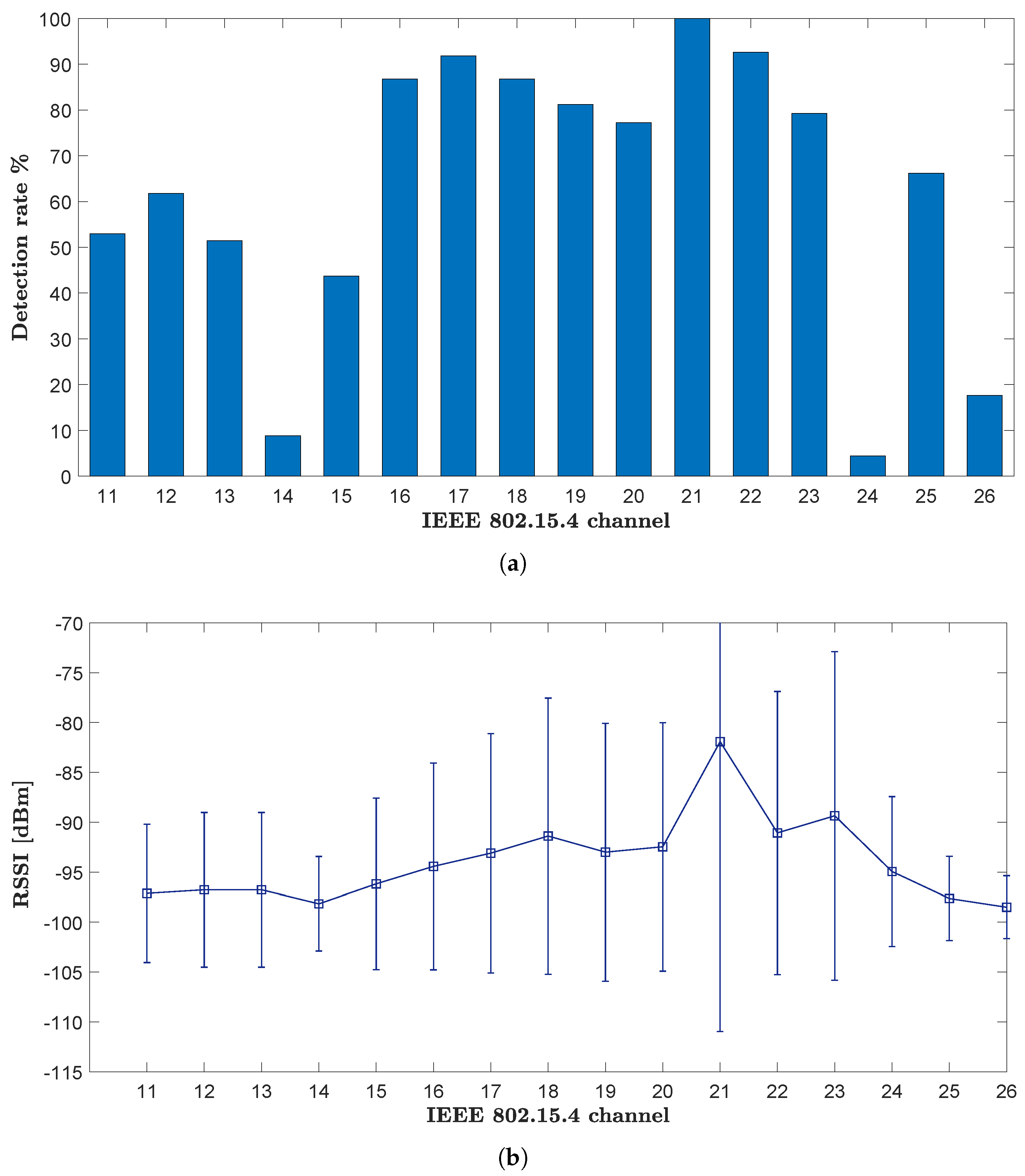
In Figure 9, we show both the classification rate at Location C for a MWO and the average RSSI value and the standard deviation for the collected test data. As mentioned beforehand, while the RF leakage from MWO spans all along the 2.4-GHz ISM band, the detection accuracy presents considerable variations along the 16 IEEE 802.15.4 channels. In particular, the eight channels 16–23 seem to offer the best chance for microwave detection, while Channel 21 shows the maximum classification accuracy. This is because, as reported in [36] and the references therein, the residential MWOs have an emission peak frequency around 2.45 GHz, which corresponds to Channel 20 in the IEEE 802.15.4 mapping. In this case, we are likely to be experiencing an MWO with center emission frequency at 2.455 GHz, which consequently triggers a very high detection rate on Channel 21. Nevertheless, since the emission pattern may vary from model to model, the channel-specific performance is expected to vary from the one shown in Figure 9. In any case, for any model, the average detection accuracy is expected to remain consistent, since there will always be a region of maximum emission inside the ISM band of interest. For the aforementioned reasons, a reasonable approach for channel sensing could be to perform the sensing on Channel 20 or on the adjacent channels in order to maximize the classification accuracy.
8. Discussion
8.1. The Influence of Sampling Window Length
In this section, we analyze the impact of different sampling window lengths on the classification accuracy of the three channel status classes of interest. The different sampling windows are tested by varying the number of samples included in the feature extraction process, as described in Section 5. In Figure 10, we show the curves for the average full-spectrum classification accuracy of IEEE 802.11 interference for sampling windows spanning from 50 ms–400 ms. We additionally show the curves representing the misclassification rate in order to highlight how the separation between classes is influenced by the sampling window.
It is interesting to note that the proposed classifier was not able to ensure proper separation between the classes IEEE 802.11 and IFC when the sampling window is 50 ms, while the accuracy increases rapidly as approaches 200 ms, stabilizing around . This behavior is mainly driven by the dynamics of IEEE 802.11 silent networks. Since a silent network shows by definition a low or null rate of exchanged data packets, due to a limited number of associated terminals, the on-air transmission is mainly due to the beacons emitted by the access point. Since the beacon period for all of the networks in experiments was set to the default value of 102.4 ms, a short sampling window can result in an increased possibility of missing the sensing of the beacon, which in turn reflects an insufficient separation between the vectors representing the IFC class and the IEEE 802.11 class in the employed -dimensional feature space. Nevertheless, thanks to the supervised-learning structure of the classifier, the proposed method allows the detection an IEEE 802.11 network with good accuracy in less than two beacon periods, while in concurrent approaches (e.g., [26]), the channel should be sensed for the time of several beacon periods in order to maximize the detection rate. The curves representing the classification rate for the IFCs are shown in Figure 11.
In the case of IFC, the classification accuracy trend is opposite with respect to the IEEE 802.11 interference classification. This can be simply explained by the fact that shorter observation windows will in turn mean a lower probability of encountering amplitude fluctuations of the background noise, which can potentially drift the feature vector in the decisional zone of IEEE 802.11 and MWO classes. Despite this fact, the IFC classification rate was reported consistently above , even for sampling windows greater than 200 ms, while we observed an increase of MWO and IEEE 802.11 misclassification, for the reason just described.
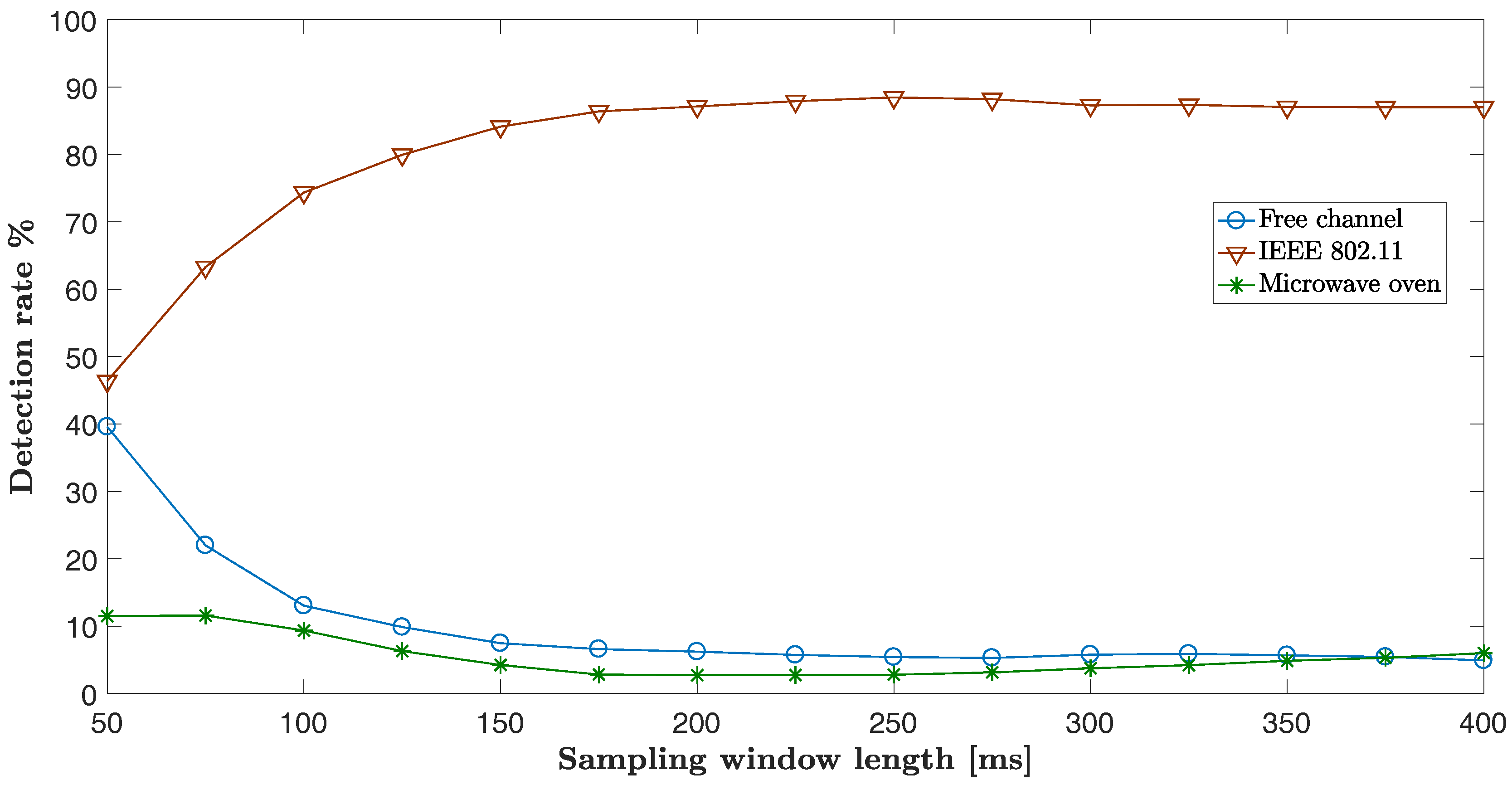
In Figure 12, we show the full-spectrum classification accuracy for MWO interference.
The figure shows insufficient separation between the classes MWO and IEEE 802.11 for 50 ms, while increasing the sampling time improves the classification accuracy, even if the improvement is significantly slower with respect to the case of IEEE 802.11 interference. This in turn means that in order to maximize the separation between classes, a sampling window of 250 ms is required so that the selected features can emerge with sufficient clarity and ensure a full spectrum classification accuracy greater than 82%. As discussed in Section 7, this behavior is due to the similarity of the temporal features of IEEE 802.11 signals in the case of active networks and the RF leakage of MWO.
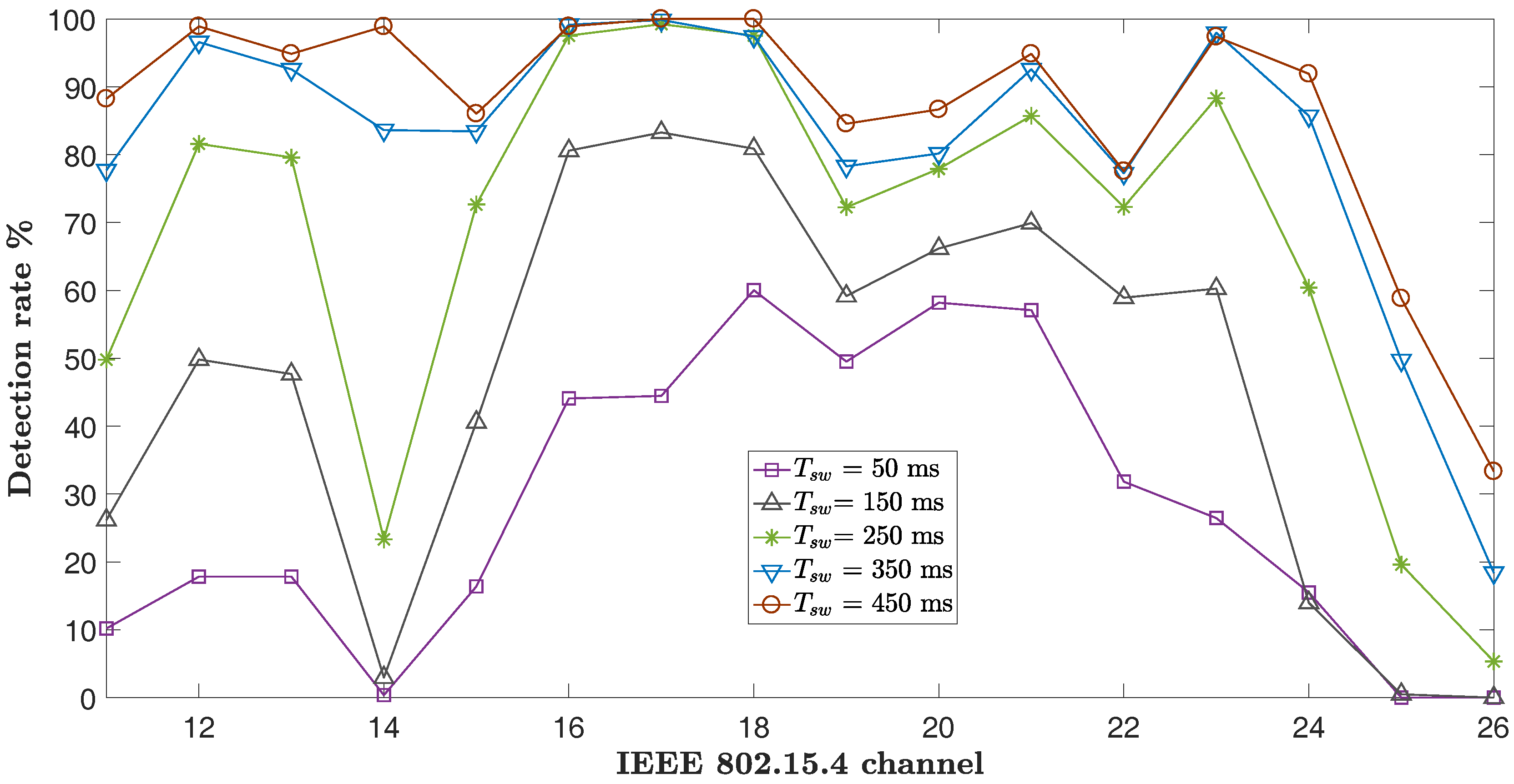
In Figure 13, we finally show the effects of different sampling windows on the in-channel detection accuracy for MWO at Location C.
From the plot, we observe that the classification accuracy is monotonically increasing for all of the channels, meaning that longer sampling windows are always beneficial for MWO detection. It can also be noted that the classification accuracy dip on Channel 14 and on Channel 24 experiences a significant improvement when the sampling window approaches 350 ms, giving a hint about the bursty time distribution of the RSSI samples on the side spectrum of MWO leakage.
8.2. Hardware-Related Considerations
Since COTS WSN nodes are low-power devices with resource-constrained hardware, particular attention has to be paid when implementing a complex methods on these platforms. In this section, we discuss how certain characteristics of the selected hardware (i.e., CC2420-equipped TelosB motes) influence the spectrum-sensing task and consequently the applicability and performance of the proposed classification method.
8.2.1. The Role of Node Calibration
It is a well-known fact that different CC2420-based devices can show variation in the nominal response of the RSSI curve. Since the core of the proposed method is based on RSSI sampling and threshold-based features, it is of primary importance to analyze if these variations can hamper the performance of the classifier. In their work, Chen et al. [41] showed that these variations are due to two different phenomena: a non-linearity in the CC2420 RSSI response curve and the presence of a node-dependent offset. While the first phenomenon is of minor relevance, since the non-linear and non-injective regions do not influence significantly the RSSI curve (which remains mostly linear), a consistent offset of ±6 dB is reported among different nodes.
We have tested several different TelosB nodes, sampling IEEE 802.15.4 Channel 26 in a radio-controlled environment to determine both the amplitude distribution and the mean of the collected RSSI traces for different nodes. As shown in Figure 14, we have observed a maximum RSSI offset of ±5 dB.
We carried out an analysis of the influence of the RSSI offset existing between the network device deployed for channel sensing and the device used for preliminary training set collection. In Figure 15, we show the impact of RSSI offset on the classification accuracy of the three targeted interference classes.
As can be observed, performing the channel sensing using a node with a consistent RSSI offset can greatly hamper the performance of the classifier, also considering that the offset between two nodes could theoretically span up to 12 dB. Even an offset of 5 dB, such as the one reported in our node set, can decrease the performance of both IEEE 802.11 andMWO classification up 15–20%, rendering a node calibration process a relevant step from the perspective of safeguarding the performance of the proposed approach. Fortunately, this process is straightforward, since as shown in [41], only a simple noise-floor-based RSSI offset calculation and compensation is needed. In the proposed approach, for example, once the RSSI offset is acquired, the offset compensation can be simply implemented by employing a software-based adaptation of the energy-threshold used for the feature-extraction task.
8.2.2. Assessing the Timeliness of the Sampling Process
In order to discuss the feasibility of the proposed sensing scheme with respect to the employed COTS hardware platform, we monitor and analyze the delay generated by the various operations needed to perform the in-node channel sensing. In Figure 16, we show the partial duration of the tasks implemented in TelosB motes in order to acquire and store the RSSI samples. Two of the most demanding tasks in terms of delay are the request for accessing and releasing the I/O resources, requiring 212 s and 74 s, respectively. In addition, the tasks of setting the CSn (chip select) pin for reading the CC2420 RSSI register lasts 12 s, while the actual operation of sampling the value of RSSI register takes 112 s to be completed.
The total delay for collecting and storing one sample is then 429 s, while we use a sampling frequency of 2 kHz, corresponding to a 500 s sampling period. With the current approach, the sampling frequency could be theoretically pushed up to 4.6 kHz if the CC2420 resources are not released until the end of the whole sampling process. In other approaches (e.g., [26]), the implementation for the channel sensing in Contiki OS allows for a sampling rate up to 8.13 kHz. Nevertheless, a higher sampling frequency means more data to process, as well as a more stressful and energy-consuming sampling process. Therefore, in this work, we have employed a more relaxed sampling timing, while we rely on the approach of an advanced classification algorithm, in order to maintain high classification performance while ensuring a lower memory footprint.
9. Conclusions
In this paper, we present a novel scheme employing machine learning methods for cross-technology interference classification in IWSAN. The proposed method employs a three-step classifier composed of a lightweight feature-extraction process, a preliminary classification stage employing four SVMs and a final decisor, allowing for classification among interference from IEEE 802.11 networks, microwave ovens, as well as the presence of interference-free channels. The tests conducted in industrial environments, including a wide range of interference scenarios, show an average classification accuracy of and up to for IEEE 802.11 active networks, with a channel sensing time of 300 ms. The memory footprint of the samples collected in this sensing time remains below 600 bytes per channel thanks to the limited sampling frequency. The extremely short time required for sensing renders the developed solution a promising candidate for the adoption in superframe-based TSCH networks by means of spectrum-sensing-reserved timeslots. In this paper, we have also highlighted the fundamental influence of device calibration on the performance of spectrum-sensing-based methods using COTS WSN hardware, which is a matter often overlooked in related literature. In particular, it is shown that the classification accuracy of the proposed solution is significantly influenced by the intrinsic hardware variations.
We leave to future works further investigations on the potentialities of SVM-based-methods for interference classification in IWSAN. Other notable aspects of interest are the inclusion of the channel-sensing and classification mechanism in a TSCH network and a run-time assessment of the solution, as well as the development of interference mitigation strategies.
Acknowledgments
The authors would like to thank Imerys Mineral AB for the access to their production plant in Sundsvall and R.Rondón from Mid Sweden University for the helpful feedback.
Author Contributions
S.G. conceived and implemented the proposed method; S.G and A.M. designed and conducted the experiments; S.G. analyzed the data. M.G. supervised the overall work. S.G., A.M. wrote the paper. All authors contributed in discussing and revising the manuscript.
Conflicts of Interest
The authors declare no conflict of interest.
References
- Prathap, U.; Shenoy, P.D.; Venugopal, K.R.; Patnaik, L.M. Wireless Sensor Networks Applications and Routing Protocols: Survey and Research Challenges. In Proceedings of the 2012 International Symposium on Cloud and Services Computing, Mangalore, India, 17–18 December 2012; pp. 49–56. [Google Scholar]
- Đurišić, M.P.; Tafa, Z.; Dimić, G.; Milutinović, V. A survey of military applications of wireless sensor networks. In Proceedings of the 2012 Mediterranean Conference on Embedded Computing (MECO), Bar, Montenegro, 19–21 June 2012; pp. 196–199. [Google Scholar]
- Mangali, N.K.; Kota, V.K. Health monitoring systems: An energy efficient data collection technique in wireless sensor networks. In Proceedings of the 2015 International Conference on Microwave, Optical and Communication Engineering (ICMOCE), Bhubaneswar, India, 18–20 December 2015; pp. 130–133. [Google Scholar]
- Benkhelifa, I.; Nouali-Taboudjemat, N.; Moussaoui, S. Disaster Management Projects Using Wireless Sensor Networks: An Overview. In Proceedings of the 2014 28th International Conference on Advanced Information Networking and Applications Workshops, Victoria, BC, Canada, 13–16 May 2014; pp. 605–610. [Google Scholar]
- IEEE Standard for Information technology—Local and metropolitan area networks—Specific requirements—Part 15.4: Wireless Medium Access Control (MAC) and Physical Layer (PHY) Specifications for Low Rate Wireless Personal Area Networks (WPANs); IEEE Std 802.15.4-2006; IEEE: New York, NY, USA, 2006.
- Åkerberg, J.; Gidlund, M.; Björkman, M. Future research challenges in wireless sensor and actuator networks targeting industrial automation. In Proceedings of the 2011 9th IEEE International Conference on Industrial Informatics, Lisbon, Portugal, 26–29 July 2011; pp. 410–415. [Google Scholar]
- Galloway, B.; Hancke, G. Introduction to Industrial Control Networks. IEEE Commun. Surv. Tutor. 2013, 15, 860–880. [Google Scholar] [CrossRef]
- Rappaport, T.S. Indoor radio communications for factories of the future. IEEE Commun. Mag. 1989, 27, 15–24. [Google Scholar] [CrossRef]
- Gwarek, W.K.; Celuch-Marcysiak, M. A review of microwave power applications in industry and research. In Proceedings of the 15th International Conference on Microwaves, Radar and Wireless Communications (IEEE Cat. No.04EX824), Warsaw, Poland, 17–19 May 2004; Volume 3, pp. 843–848. [Google Scholar]
- Sikora, A. Wireless Personal and Local Area Networks; Wiley: Chichester, UK; Hoboken, NJ, USA, 2003. [Google Scholar]
- Liang, C.J.M.; Priyantha, N.B.; Liu, J.; Terzis, A. Surviving Wi-Fi Interference in Low Power ZigBee Networks. In Proceedings of the 8th ACM Conference on Embedded Networked Sensor Systems, Zürich, Switzerland, 3–5 November 2010; ACM: New York, NY, USA, 2010; pp. 309–322. [Google Scholar]
- Yang, D.; Xu, Y.; Gidlund, M. Wireless Coexistence between IEEE 802.11- and IEEE 802.15.4-Based Networks: A Survey. Int. J. Distrib. Sens. Netw. 2011, 7, 912152. [Google Scholar] [CrossRef]
- Hermans, F.; Rensfelt, O.; Voigt, T.; Ngai, E.; Norden, L.A.; Gunningberg, P. SoNIC: Classifying Interference in 802.15.4 Sensor Networks. In Proceedings of the 12th International Conference on Information Processing in Sensor Networks (IPSN ’13), Philadelphia, PA, USA, 8–11 April 2013; ACM: New York, NY, USA, 2013; pp. 55–66. [Google Scholar]
- HART Communication Protocol Specification, Revision 7.4; Technical Report; HART Communication Foundation: Austin, TX, USA, 2012.
- Wireless Systems for Industrial Automation: Process Control and Related Applications; ISA 100.11a-2011; International Society of Automation: Research Triangle Park, NC, USA, 2011.
- Industrial Communication Networks—Fieldbus Specifications—WIA-PA Communication Network and Communication Profile; IEC 62601; International Electrotechnical Commission: Geneva, Switzerland, 2011.
- Yucek, T.; Arslan, H. A survey of spectrum sensing algorithms for cognitive radio applications. IEEE Commun. Surv. Tutor. 2009, 11, 116–130. [Google Scholar] [CrossRef]
- Brown, J.; Roedig, U.; Boano, C.A.; Römer, K. Estimating packet reception rate in noisy environments. In Proceedings of the 39th Annual IEEE Conference on Local Computer Networks Workshops, Edmonton, AB, Canada, 8–11 September 2014; pp. 583–591. [Google Scholar]
- Zacharias, S.; Newe, T.; O’Keeffe, S.; Lewis, E. A Lightweight Classification Algorithm for External Sources of Interference in IEEE 802.15.4-Based Wireless Sensor Networks Operating at the 2.4 GHz. Int. J. Distrib. Sens. Netw. 2014, 10, 265286. [Google Scholar] [CrossRef]
- Zhou, R.; Xiong, Y.; Xing, G.; Sun, L.; Ma, J. ZiFi: wireless LAN discovery via ZigBee interference signatures. In Proceedings of the sixteenth annual international conference on Mobile computing and networking, Chicago, IL, USA, 20–24 September 2010; ACM: New York, NY, USA, 2010; pp. 49–60. [Google Scholar]
- Gao, Y.; Niu, J.; Zhou, R.; Xing, G. ZiFind: Exploiting cross-technology interference signatures for energy-efficient indoor localization. In Proceedings of the 2013 Proceedings IEEE INFOCOM, Turin, Italy, 14–19 April 2013; pp. 2940–2948. [Google Scholar]
- Choi, J. WidthSense: Wi-Fi Discovery via Distance-based Correlation Analysis. IEEE Commun. Lett. 2016, 21, 422–425. [Google Scholar] [CrossRef]
- Petrova, M.; Wu, L.; Mahonen, P.; Riihijarvi, J. Interference Measurements on Performance Degradation between Colocated IEEE 802.11 g/n and IEEE 802.15.4 Networks. In Proceedings of the Sixth International Conference on Networking (2007. ICN ’07), Sainte-Luce, France, 22–28 April 2007; p. 93. [Google Scholar]
- Hossian, M.M.A.; Mahmood, A.; Jäntti, R. Channel ranking algorithms for cognitive coexistence of IEEE 802.15.4. In Proceedings of the 2009 IEEE 20th International Symposium on Personal, Indoor and Mobile Radio Communications, Tokyo, Japan, 13–16 September 2009; pp. 112–116. [Google Scholar]
- ZigBee Standards Organization. ZigBee Specifications; ZigBee Standards Organization: San Ramon, CA, USA, 2012; pp. 1–622. [Google Scholar]
- Zacharias, S.; Newe, T.; O’Keeffe, S.; Lewis, E. 2.4 GHz IEEE 802.15.4 channel interference classification algorithm running live on a sensor node. In Proceedings of the 2012 IEEE Sensors, Taipei, Taiwan, 28–31 Octorber 2012; pp. 1–4. [Google Scholar]
- Iyer, V.; Hermans, F.; Voigt, T. Detecting and Avoiding Multiple Sources of Interference in the 2.4 GHz Spectrum. In Proceedings of the12th European Conference on Wireless Sensor Networks (EWSN), Porto, Portugal, 9–11 February 2015; Abdelzaher, T., Pereira, N., Tovar, E., Eds.; Springer International Publishing: Cham, Switzerland, 2015; pp. 35–51. [Google Scholar]
- Ansari, J.; Ang, T.; Mähönen, P. WiSpot: fast and reliable detection of Wi-Fi networks using IEEE 802.15.4 radios. In Proceedings of the 9th ACM International Symposium on Mobility Management and Wireless Access, Miami, FL, USA, 31 October–4 November 2011; ACM: New York, NY, USA, 2011; pp. 35–44. [Google Scholar]
- Chowdhury, K.R.; Akyildiz, I.F. Interferer Classification, Channel Selection and Transmission Adaptation for Wireless Sensor Networks. In Proceedings of the 9th IEEE International Conference on Communications (ICC ’09), Dresden, Germany, 14–18 June 2009; pp. 1–5. [Google Scholar]
- Rayanchu, S.; Patro, A.; Banerjee, S. Airshark: Detecting non-WiFi RF Devices Using Commodity WiFi Hardware. In Proceedings of the 2011 ACM SIGCOMM Conference on Internet Measurement Conference (IMC ’11), Berlin, Germany, 2–4 November 2011; ACM: New York, NY, USA, 2011; pp. 137–154. [Google Scholar]
- Weng, Z.; Orlik, P.; Kim, K.J. Classification of wireless interference on 2.4 GHz spectrum. In Proceedings of the 2014 IEEE Wireless Communications and Networking Conference (WCNC), Istanbul, Turkey, 6–9 April 2014; pp. 786–791. [Google Scholar]
- Hermans, F.; Larzon, L.A.; Rensfelt, O.; Gunningberg, P. A Lightweight Approach to Online Detection and Classification of Interference in 802.15.4-based Sensor Networks. SIGBED Rev. 2012, 9, 11–20. [Google Scholar] [CrossRef]
- Nicolas, C.; Marot, M. Dynamic link adaptation based on coexistence-fingerprint detection for WSN. In Proceedings of the 2012 11th Annual Mediterranean Ad Hoc Networking Workshop (Med-Hoc-Net), Ayia Napa, Cyprus, 19–22 June 2012; pp. 90–97. [Google Scholar]
- Barać, F.; Gidlund, M.; Zhang, T. Ubiquitous, Yet Deceptive: Hardware-Based Channel Metrics on Interfered WSN Links. IEEE Trans. Veh. Technol. 2015, 64, 1766–1778. [Google Scholar] [CrossRef]
- Zheng, X.; Cao, Z.; Wang, J.; He, Y.; Liu, Y. ZiSense: Towards Interference Resilient Duty Cycling in Wireless Sensor Networks. In Proceedings of the 12th ACM Conference on Embedded Network Sensor Systems, (SenSys ’14), Memphis, TN, USA, 3–6 November 2014; ACM: New York, NY, USA, 2014; pp. 119–133. [Google Scholar]
- Rondeau, T.W.; D’Souza, M.F.; Sweeney, D.G. Residential microwave oven interference on Bluetooth data performance. IEEE Trans. Consum. Electron. 2004, 50, 856–863. [Google Scholar] [CrossRef]
- Bishop, C.M. Pattern Recognition and Machine Learning (Information Science and Statistics); Springer: Secaucus, NJ, USA, 2006. [Google Scholar]
- Boyd, S.; Vandenberghe, L. Convex Optimization; Cambridge University Press: New York, NY, USA, 2004. [Google Scholar]
- Crossbow TelosB Mote Plattform, Datasheet. Available online: http://www.willow.co.uk/TelosB_Datasheet.pdf (accessed on 16 June 2017).
- Texas Instruments CC2420 - 2.4 GHz IEEE 802.15.4/ZigBee-ready RF Transceiver. Available online: http://www.ti.com/lit/ds/symlink/cc2420.pdf (accessed on 16 June 2017).
- Chen, Y.; Terzis, A. On the mechanisms and effects of calibrating RSSI measurements for 802.15.4 radios. In Proceedings of the 7th European conference on Wireless Sensor Networks, Coimbra, Portugal, 17–19 February 2010; Springer: Berlin/Heidelberg, Germany, 2010; pp. 256–271. [Google Scholar]
- Metageek Wi-Spy Chanalizer. Available online: http://files.metageek.net/marketing/data-sheets/MetaGeek_Wi-Spy-Chanalyzer_DataSheet.pdf (accessed on 16 June 2017).
- Boano, C.A.; Voigt, T.; Noda, C.; Römer, K.; Zúñiga, M. JamLab: Augmenting sensornet testbeds with realistic and controlled interference generation. In Proceedings of the 10th ACM/IEEE International Conference on Information Processing in Sensor Networks, Chicago, IL, USA, 12–14 April 2011; pp. 175–186. [Google Scholar]
Figure 1.
The 2.4-GHz industrial, scientific and medical (ISM) spectrum. Channel allocation for heterogeneous technologies with RF emissions within the band: IEEE 802.11, Bluetooth, microwave oven (MWO), IEEE 802.15.4.
Figure 1.
The 2.4-GHz industrial, scientific and medical (ISM) spectrum. Channel allocation for heterogeneous technologies with RF emissions within the band: IEEE 802.11, Bluetooth, microwave oven (MWO), IEEE 802.15.4.
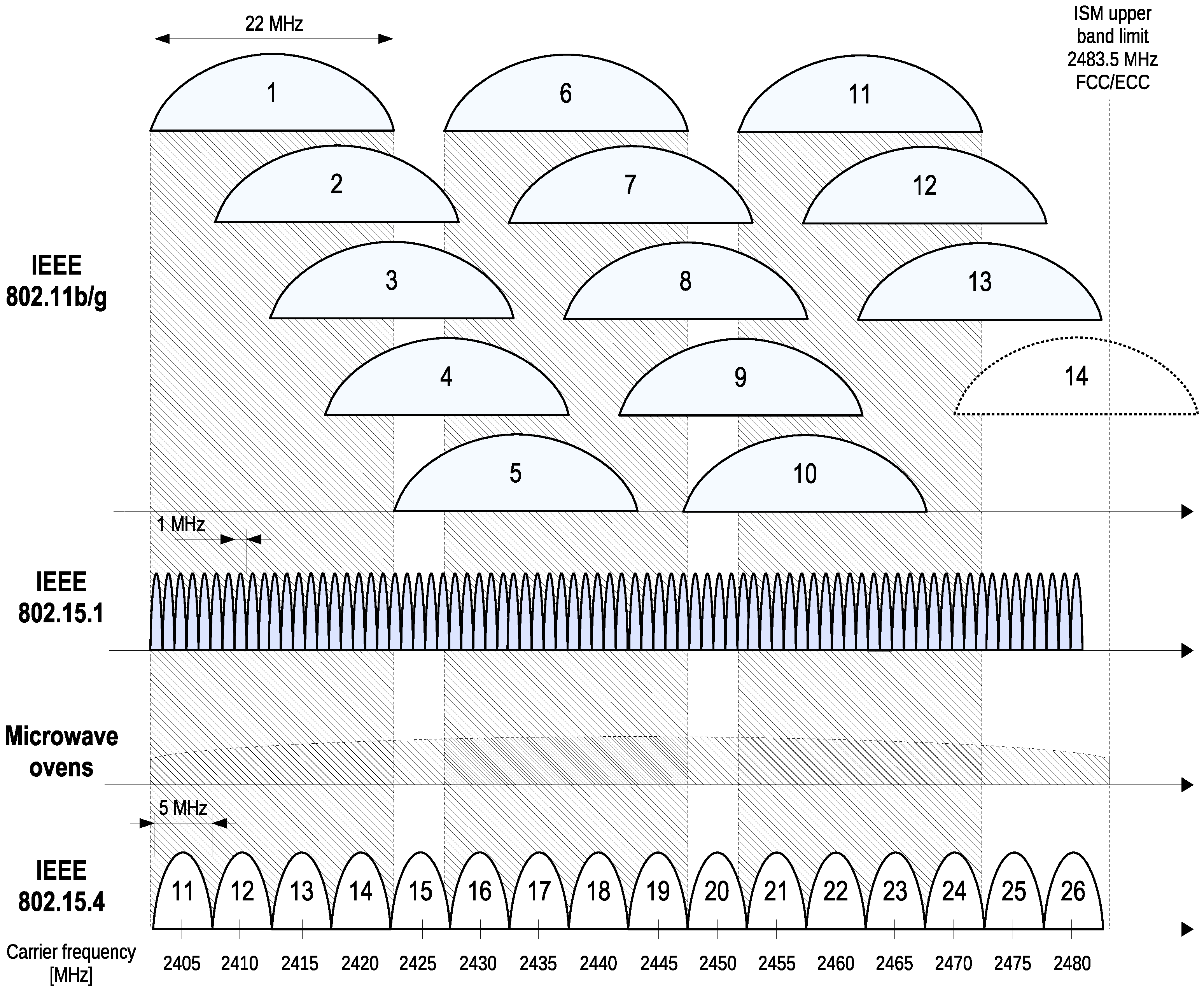
Figure 2.
An overview of interference classification methods.

Figure 3.
Setup of the support vector machine (SVM)-based interference classifier.

Figure 4.
Details of the decisor for the proposed detection algorithm. The logic input signals are generated by the four SVMs in Figure 3.
Figure 4.
Details of the decisor for the proposed detection algorithm. The logic input signals are generated by the four SVMs in Figure 3.

Figure 5.
Two of the selected experimental environments. (a) Location A: industrial plant; (b) Location B: mechanical workshop.
Figure 5.
Two of the selected experimental environments. (a) Location A: industrial plant; (b) Location B: mechanical workshop.

Figure 6.
Experimental setup for the collection of training data for IEEE 802.11 interference detection.
Figure 6.
Experimental setup for the collection of training data for IEEE 802.11 interference detection.
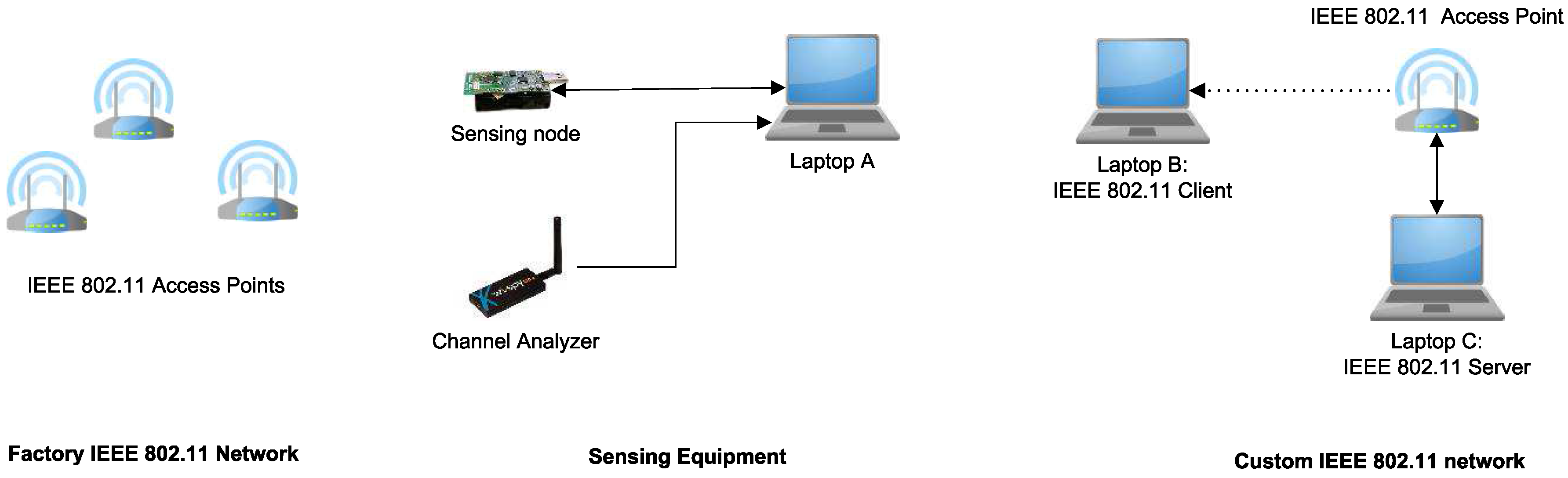
Figure 7.
Location A, three IEEE 802.11 access point operating on IEEE 802.11 Channels . (a) Channel-specific detection rate at Location A for the sampling window length of 150 ms; (b) IEEE 802.11 power spectral density (PSD) as observed by the channel analyzer.
Figure 7.
Location A, three IEEE 802.11 access point operating on IEEE 802.11 Channels . (a) Channel-specific detection rate at Location A for the sampling window length of 150 ms; (b) IEEE 802.11 power spectral density (PSD) as observed by the channel analyzer.
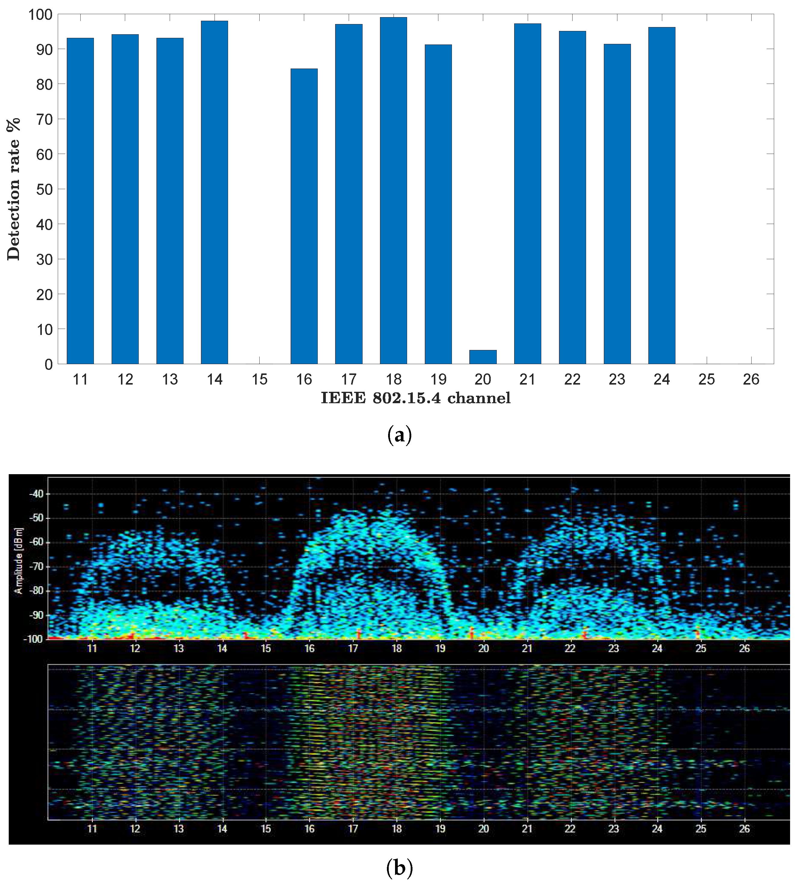
Figure 8.
Location B, multiple IEEE 802.11 access points operating on Channels . (a) Channel-specific detection rate at Location B for a sampling window length of 150 ms.; (b) IEEE 802.11 power spectral density (PSD) as observed by the channel analyzer.
Figure 8.
Location B, multiple IEEE 802.11 access points operating on Channels . (a) Channel-specific detection rate at Location B for a sampling window length of 150 ms.; (b) IEEE 802.11 power spectral density (PSD) as observed by the channel analyzer.
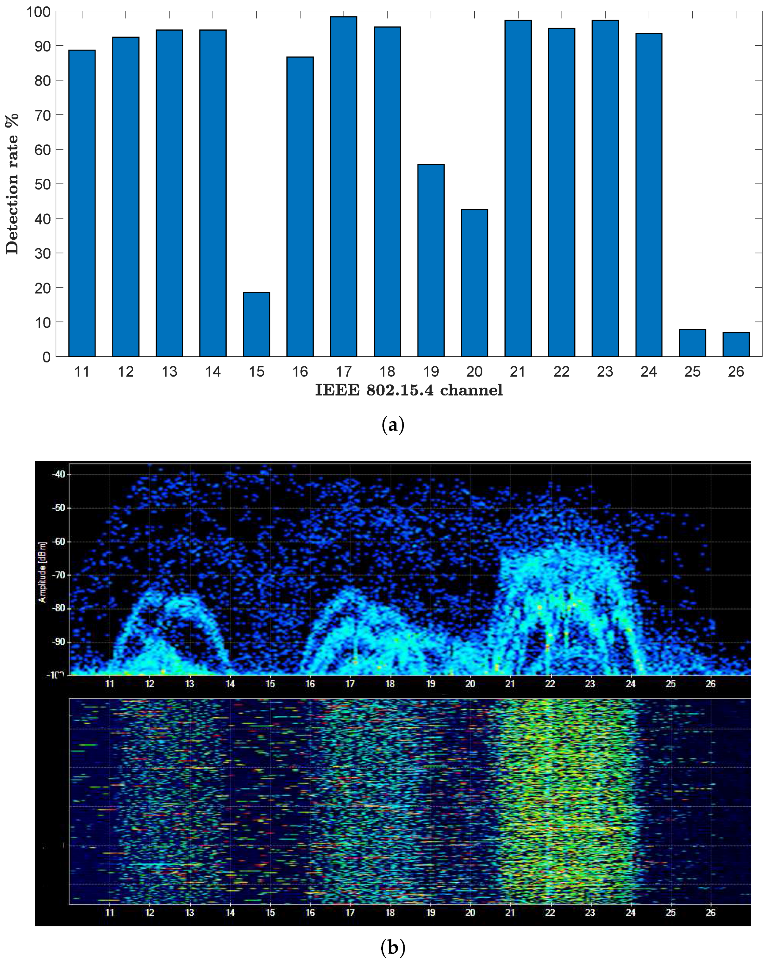
Figure 9.
Location C, classification results for a sampling window length of 300 ms. (a) Channel-specific microwave oven detection rate; (b) average and standard deviation of RSSI traces collected in proximity of the tested microwave oven.
Figure 9.
Location C, classification results for a sampling window length of 300 ms. (a) Channel-specific microwave oven detection rate; (b) average and standard deviation of RSSI traces collected in proximity of the tested microwave oven.

Figure 10.
Average full-spectrum detection rate for IEEE 802.11 scenarios for different sampling window lengths.
Figure 10.
Average full-spectrum detection rate for IEEE 802.11 scenarios for different sampling window lengths.

Figure 11.
Average full-spectrum detection rate for interference-free scenarios for different sampling window lengths.
Figure 11.
Average full-spectrum detection rate for interference-free scenarios for different sampling window lengths.
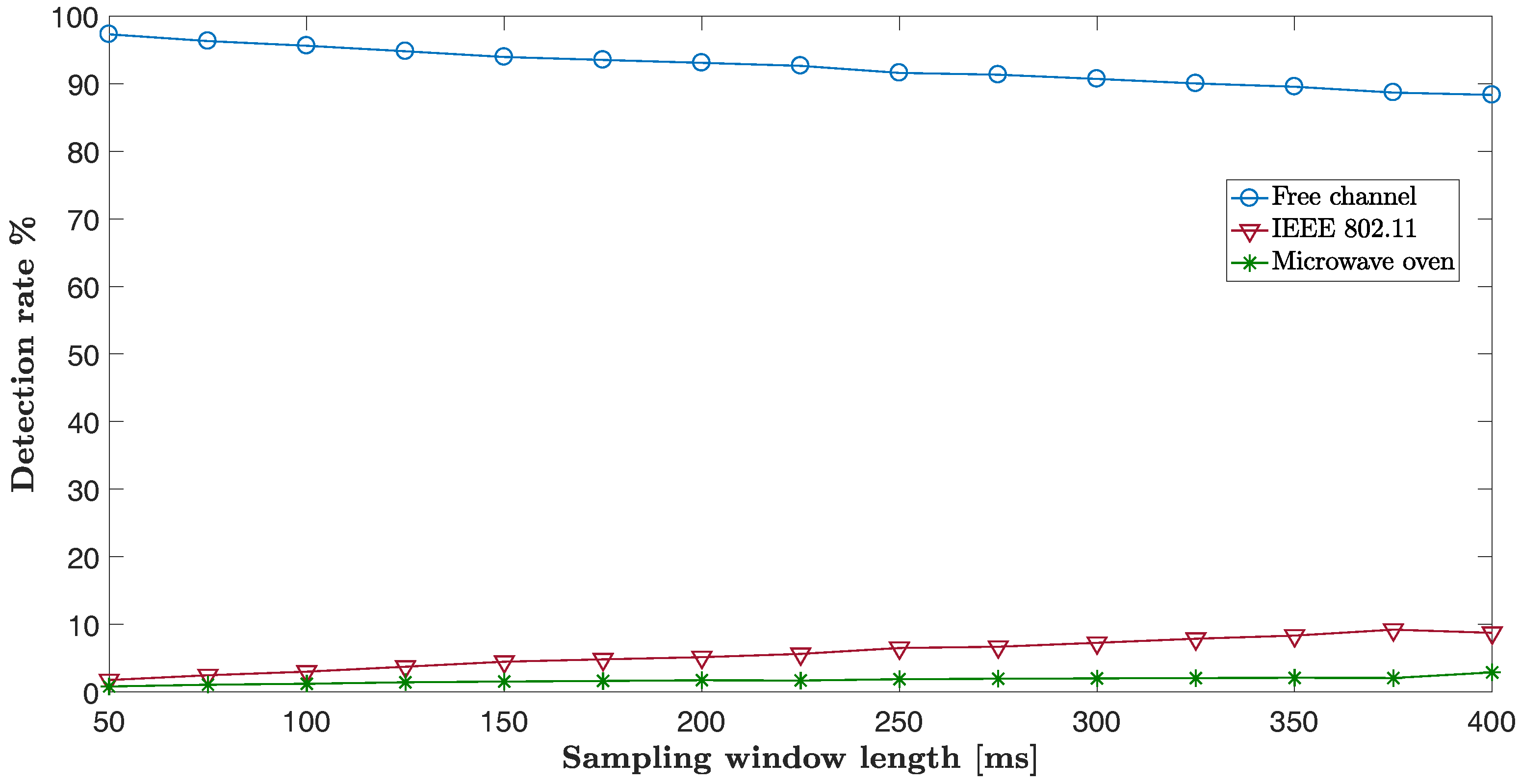
Figure 12.
Average full-spectrum detection rate for interference from MWO for different sampling window lengths.
Figure 12.
Average full-spectrum detection rate for interference from MWO for different sampling window lengths.
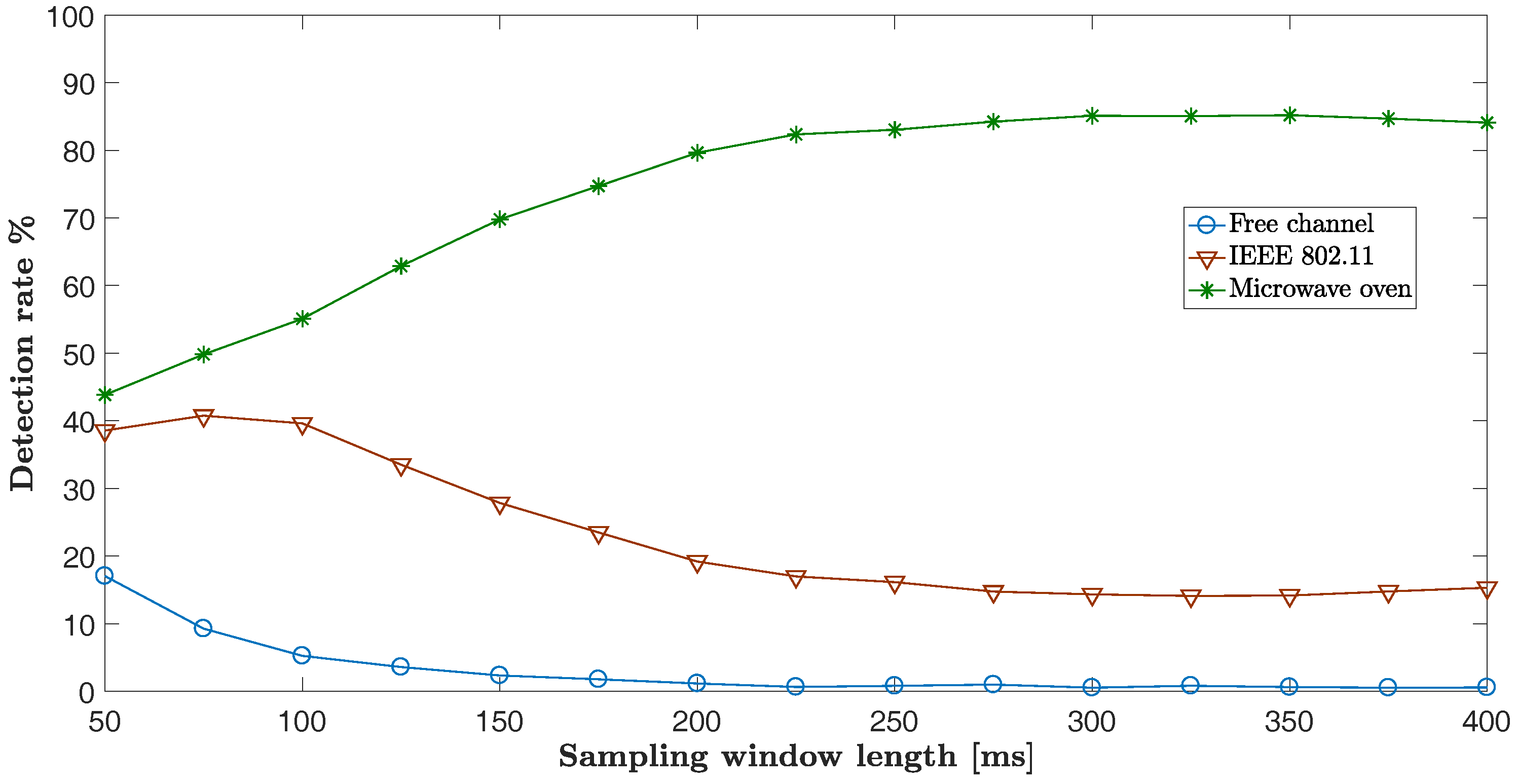
Figure 13.
Detection rate for microwave oven at Location C for different sampling window lengths. Some curves have been removed for clarity.
Figure 13.
Detection rate for microwave oven at Location C for different sampling window lengths. Some curves have been removed for clarity.

Figure 14.
The RSSI profiling process for TelosB motes. (a) Amplitude distribution of RSSI traces from background noise sensing for different CC2420 nodes. Some curves have been removed for clarity. (b) Mean of recorded RSSI sample traces.
Figure 14.
The RSSI profiling process for TelosB motes. (a) Amplitude distribution of RSSI traces from background noise sensing for different CC2420 nodes. Some curves have been removed for clarity. (b) Mean of recorded RSSI sample traces.
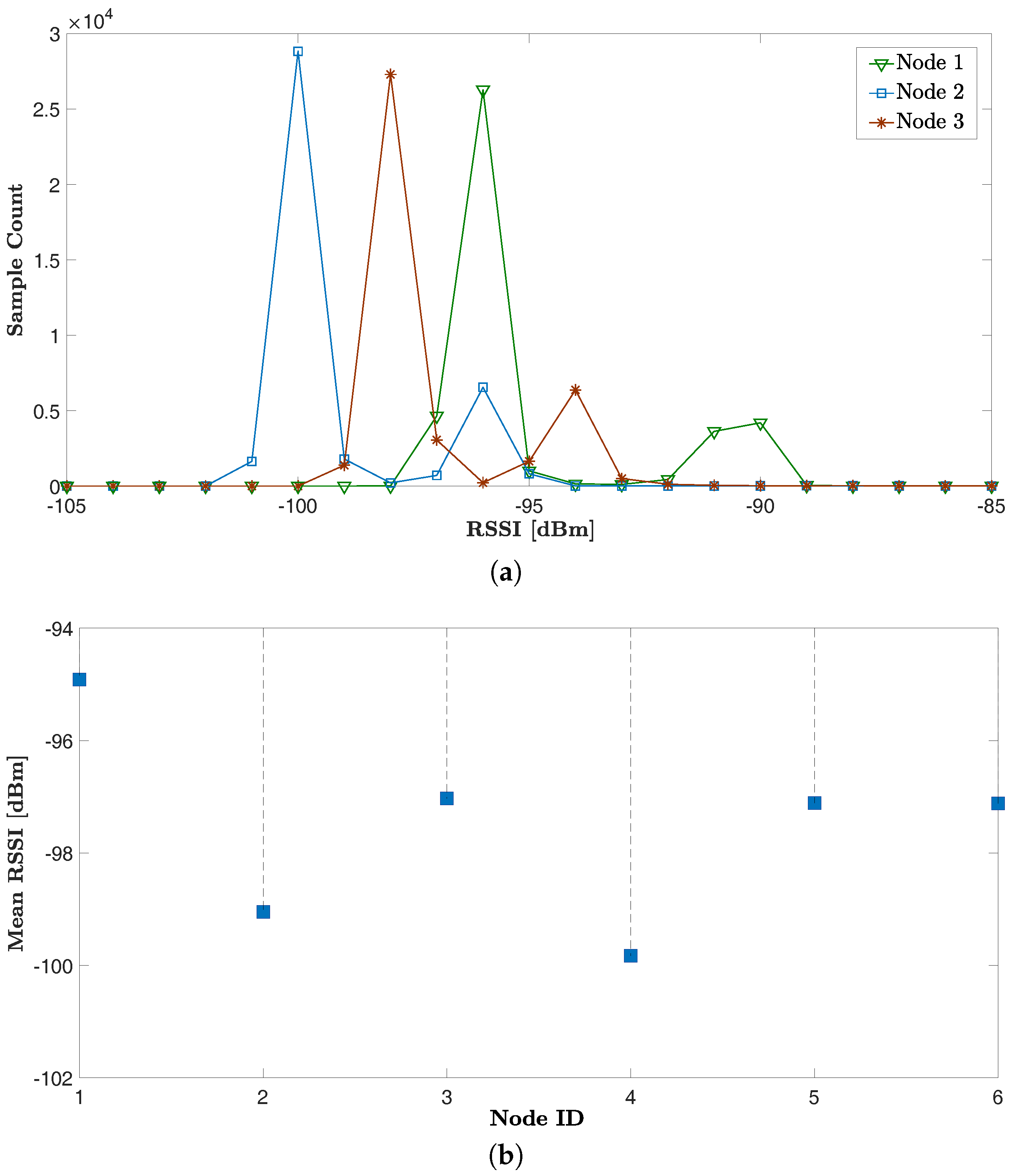
Figure 15.
Detection accuracy with respect to RSSI offset between the node used for collecting training data and the actual sensing node.
Figure 15.
Detection accuracy with respect to RSSI offset between the node used for collecting training data and the actual sensing node.
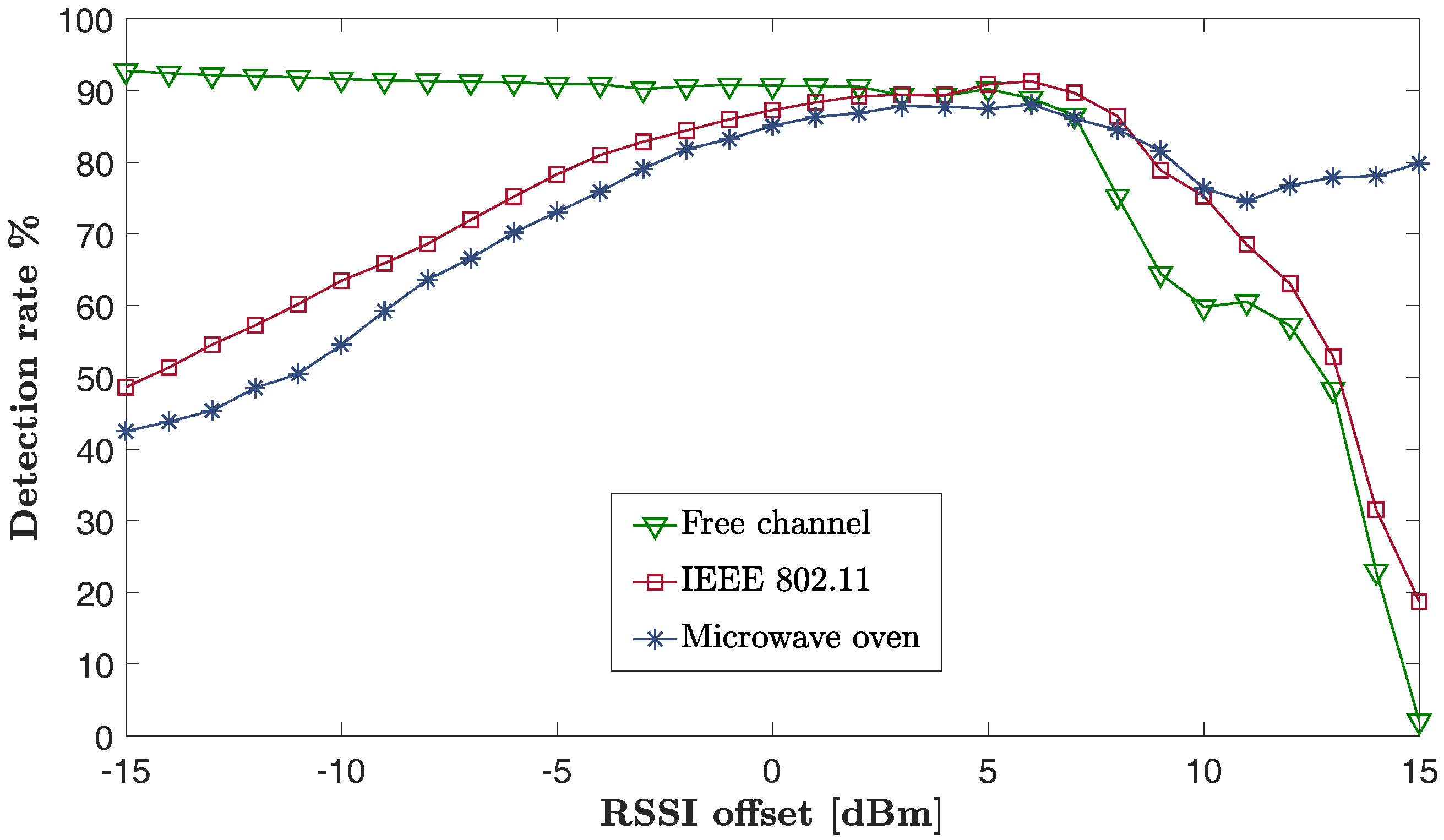
Figure 16.
Operation delays in s for the channel-sensing task implemented in TelosB motes.


Table 1.
The four interference classes in the analysis.
| Classification Outcome | |||
|---|---|---|---|
| 1 | 0 | 0 | The channel is free from the interference sources in the analysis. |
| 0 | 0 | 1 | A MWO was active during the sensing period. |
| 0 | 1 | 0 | An IEEE 802.11 network was overlapping the channel in the analysis. |
| 0 | 0 | 0 | The source of interference is unknown. |
Table 2.
Average classification accuracy for the 250 ms sampling window calculated over all of the scenarios. IFC, interference-free channel.
Table 2.
Average classification accuracy for the 250 ms sampling window calculated over all of the scenarios. IFC, interference-free channel.
| Channel Status | Detected Interference Source | |||
|---|---|---|---|---|
| IFC | IEEE 802.11 | Microwave Oven | Unknown | |
| IFC | 91.2% | 6.6% | 2.1% | 0.1% |
| IEEE 802.11 | 12.4% | 83.9% | 1.4% | 2.3% |
| Microwave Oven | 0.8% | 16.3% | 82.8% | 0.1% |
Table 3.
Average classification accuracy for the 250 ms sampling window for Location A.
| Channel Status | Detected Interference Source | |||
|---|---|---|---|---|
| IFC | IEEE 802.11 | Microwave Oven | Unknown | |
| IFC | 98.2% | 1.7% | 0.1% | 0.0% |
| IEEE 802.11 | 0.1% | 98.9% | 0.3% | 0.7% |
Table 4.
Average classification accuracy for the 250 ms sampling window for Location B.
| Channel Status | Detected Interference Source | |||
|---|---|---|---|---|
| IFC | IEEE 802.11 | Microwave Oven | Unknown | |
| IFC | 84.9% | 11.2% | 3.8% | 0.1% |
| IEEE 802.11 | 10.7% | 77.9% | 5.2% | 6.1% |
© 2017 by the authors. Licensee MDPI, Basel, Switzerland. This article is an open access article distributed under the terms and conditions of the Creative Commons Attribution (CC BY) license (http://creativecommons.org/licenses/by/4.0/).
Share and Cite
MDPI and ACS Style
Grimaldi, S.; Mahmood, A.; Gidlund, M. An SVM-Based Method for Classification of External Interference in Industrial Wireless Sensor and Actuator Networks. J. Sens. Actuator Netw. 2017, 6, 9. https://doi.org/10.3390/jsan6020009
AMA Style
Grimaldi S, Mahmood A, Gidlund M. An SVM-Based Method for Classification of External Interference in Industrial Wireless Sensor and Actuator Networks. Journal of Sensor and Actuator Networks. 2017; 6(2):9. https://doi.org/10.3390/jsan6020009
Chicago/Turabian StyleGrimaldi, Simone, Aamir Mahmood, and Mikael Gidlund. 2017. "An SVM-Based Method for Classification of External Interference in Industrial Wireless Sensor and Actuator Networks" Journal of Sensor and Actuator Networks 6, no. 2: 9. https://doi.org/10.3390/jsan6020009
Note that from the first issue of 2016, this journal uses article numbers instead of page numbers. See further details here.