Localization in Wireless Sensor Networks: A Survey on Algorithms, Measurement Techniques, Applications and Challenges

1
Department of Electronics and Communications Engineering, East West University, Dhaka 1212, Bangladesh
2
Waseda University, Tokyo 169-8050, Japan
*
Author to whom correspondence should be addressed.
J. Sens. Actuator Netw. 2017, 6(4), 24; https://doi.org/10.3390/jsan6040024
Submission received: 11 September 2017
/
Revised: 20 October 2017
/
Accepted: 24 October 2017
/
Published: 27 October 2017
Abstract
:Localization is an important aspect in the field of wireless sensor networks (WSNs) that has developed significant research interest among academia and research community. Wireless sensor network is formed by a large number of tiny, low energy, limited processing capability and low-cost sensors that communicate with each other in ad-hoc fashion. The task of determining physical coordinates of sensor nodes in WSNs is known as localization or positioning and is a key factor in today’s communication systems to estimate the place of origin of events. As the requirement of the positioning accuracy for different applications varies, different localization methods are used in different applications and there are several challenges in some special scenarios such as forest fire detection. In this paper, we survey different measurement techniques and strategies for range based and range free localization with an emphasis on the latter. Further, we discuss different localization-based applications, where the estimation of the location information is crucial. Finally, a comprehensive discussion of the challenges such as accuracy, cost, complexity, and scalability are given.
1. Introduction
In the future generation of communications networks, real-time localization and position-based services are required that are accurate, low cost, energy efficient and reliable [1,2]. Nowadays, Wireless Sensor Networks (WSNs) can be applied in many applications, such as natural resources investigation, targets tracking, unapproachable places monitoring and so forth. In these applications, the information is collected and transferred by the sensor nodes. Various applications request these sensor nodes’ location information. Moreover, the location information is also indispensable in geographic routing protocols and clustering [3,4]. All these mentioned above make localization algorithms become one of the most important issues in WSNs researches. Thus, locations of sensor nodes are important for operations in WSNs. Localization in WSNs has been intensively studied in recent years, with most of these studies relying on the condition that only a small proportion of sensor nodes, called anchor nodes, know their exact positions through GPS devices or manual configuration [5,6,7]. Other sensor nodes estimate their distances to anchor nodes and calculate positions with multi-lateration techniques. These methods provide satisfactory level of accuracy with a small proportion of anchor nodes in WSNs [8,9].
The sensor nodes are randomly deployed in inaccessible terrain by the vehicle robots or aircrafts to be used in many promising applications, such as health surveillance, battle field surveillance, environmental monitoring, coverage, routing, location service, target tracking, and rescue [10]. The Global Positioning System (GPS) or the standalone cellular systems are the most promising and accurate positioning technologies. Although they are widely accessible, the limitation of high cost and energy consuming of GPS system makes it impractical to install in every sensor node where the lifetime of a sensor node is very crucial. On the other hand, the cellular signals are interrupted in scenarios with deep shadowing effects [11]. In order to reduce the energy consumption and cost, only a few number of nodes which are called anchor or beacon nodes, contain the GPS modules. The other nodes could obtain their position information through localization method. Wireless sensor network is composed of a large number of inexpensive nodes that are densely deployed in a region of interests to measure certain phenomenon. The primary objective is to determine the location of the sensor node. Node self-localization can be classified into two categories: range based localization and range free localization. The former method uses the measured distance/angle to estimate the location. In addition, the latter method uses the connectivity or pattern matching method to estimate the location.
Various localization algorithms and methodologies have been proposed to deal with different problems in different applications. A combination of different range based techniques called hybrid positioning is a well known approach for localization that exhibits sufficient accuracy and coverage [12]. On the other hand, the localization algorithms based on hop distance and hop count based information between anchor nodes and sensor nodes are commonly known in the literature as connectivity-based or range-free algorithms. Depending on the process used to estimate the distances between the intermediate nodes, range-free algorithms may fall into two categories: heuristic, and analytical [13,14,15,16,17,18,19,20,21,22,23,24,25,26,27,28,29,30,31,32,33]. Also, range free localization algorithms are categorized based on the deployment scenarios. The categorization has been divided into four groups: (1) static sensor nodes and static anchor nodes [34,35]; (2) static sensor nodes and mobile anchor nodes [36,37]; (3) mobile sensor nodes and static anchor nodes [38,39]; and (4) mobile sensor nodes and mobile anchor nodes [40,41].
Although there are many localization techniques available to solve positioning problems in the WSNs, there are practical limits on the combination of these techniques as well as on the minimal number of anchor nodes that can be deployed in such scenarios. For example, in many situations, only one or two anchor nodes are able to communicate with the sensor nodes that need to be localized. Hence, new positioning techniques based on hybrid data fusion and/or heterogeneous access are proposed and analyzed [42].
In this paper, we present a detailed survey on recent localization techniques and concepts with their fundamental limits, challenges and applications. Although literature survey on localization techniques are available in [8,43,44,45,46,47,48], only a few papers exist that focus on range free localization techniques [49] without focusing on recent advanced techniques and applications. Thus, the survey in [45] is outdated, whereas [43] focuses only on ultrasonic positioning systems. The work in [8] describes relatively recent localization techniques but focuses only on the indoor localization techniques and briefly discusses about range free localization. The works of [46,47] review different technologies, such as Wireless Local Area Network (WLAN), used for indoor positioning. However, they do not discuss positioning neither from the perspective of energy efficiency nor from the requirement in recent applications, such as ambient assisted and health living applications. The survey in [48] provides notable categorization of various fingerprint-based outdoor positioning techniques, discussing how each method works. So, we intend to present a survey focused specially on range free techniques. Moreover, the rapid growth of various localization approaches in this field and the need for a complete and up-to-date survey of the techniques, applications and future trends, provide the motivation for this survey paper.
The remainder of this paper is organized as follows. Basic distance measurement techniques for localization in WSNs are described briefly in Section 2 with their common pitfalls and challenges. Different localization algorithms and their comparative analysis are discussed in Section 3. Section 4 describes various localization based applications. Section 5 presents various evaluation criteria for localization. Then we present perspective and challenges in range free localization algorithms in Section 6. Finally, Section 7 concludes the paper.
2. Basic Measurement Techniques for Localization in WSNs
The localization algorithms for WSNs depend on various measurement techniques. There are many factors that affect the accuracy of the localization algorithms and consequently, the choice of the localization algorithms to be used in various applications. For example, network architecture, sensor density in an area, number of anchor nodes, geometric shape of the measurement area, sensor time synchronization, and the signaling bandwidth among the sensors are the key factors to be taken into account while designing a localization algorithm. However, it is the type of measurement and the corresponding precision that fundamentally determines the accuracy of localization algorithm.
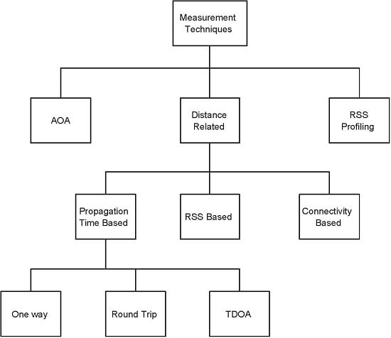
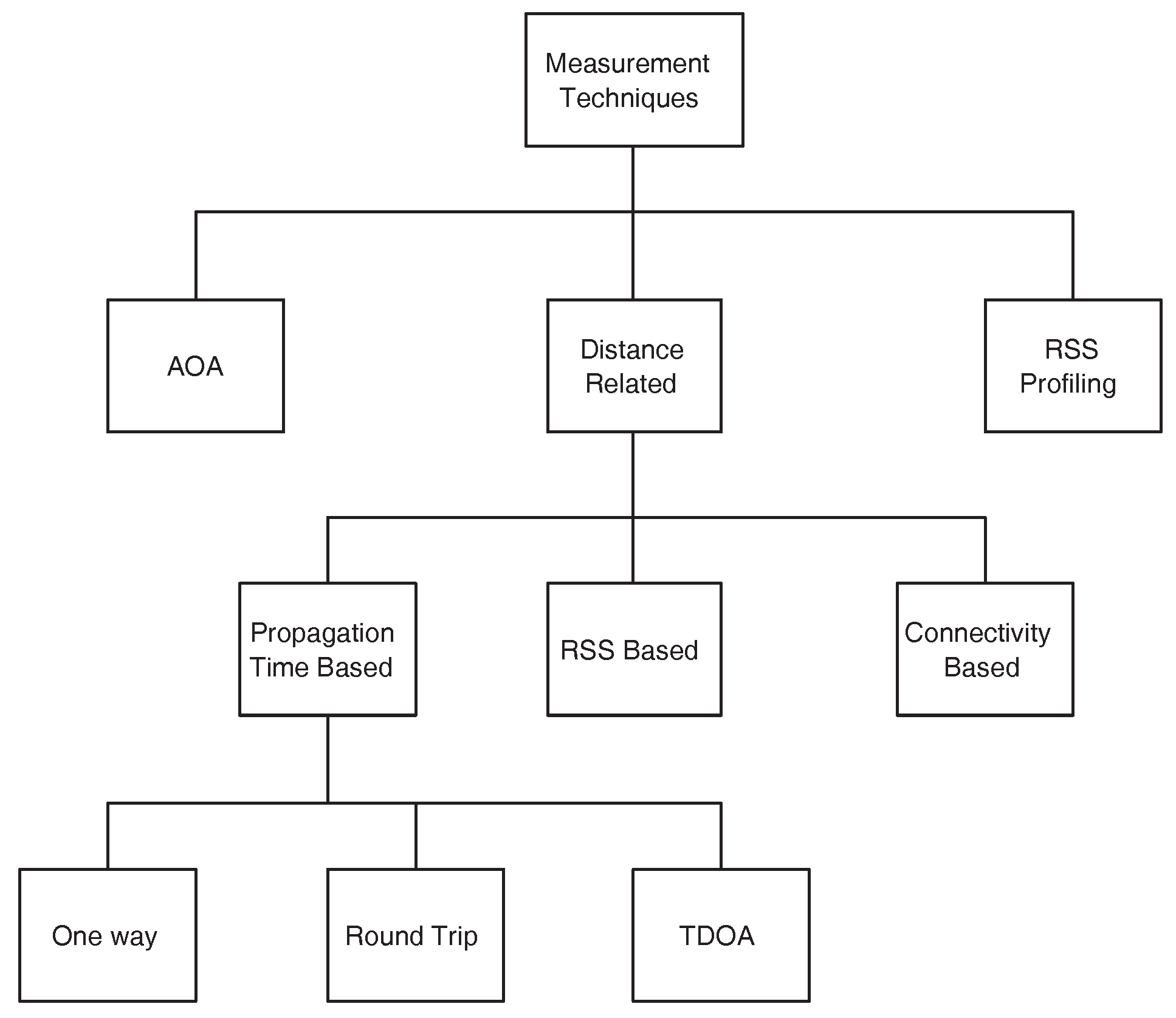
Measurement techniques in WSNs localization can be broadly classified into three categories [50]. Angle of Arrival (AOA) measurements, distance related measurements and the Radio Signal Strength (RSS) profiling techniques. Figure 1 shows the classification. In the subsequent discussion, we briefly discuss these techniques along with their limitations in different WSNs applications.
2.1. Angle of Arrival (AOA) Measurements
The AOA measurement techniques are also known as the bearing measurements or the direction of arrival measurements. The AOA measurements can be obtained from two categories of techniques: one from the receiver antenna’s amplitude response and another from the receiver antenna’s phase response. These techniques calculate the angle at which the signal arrives from the anchor node to the unknown sensor nodes. Then, the region where the unknown sensor is located, is a line having a certain angle from the anchor node. In AOA measurement techniques, at least two anchor nodes are needed to calculate the position. The localization error could be large if there is a small error in measurement. The accuracy is depended on the directionality of the antenna and measurements are further complicated by the presence of shadowing and multipath effect of the measurement environment. A multipath component from the transmitted signal may appear as a signal coming from entirely different direction and consequently causes a very large error in measurement accuracy [50]. Thus, AOA technique is of limited interest in localization unless it is used with large antenna arrays [8]. As a result, for WSNs with tiny sensor nodes, this option is not energy efficient at all.
2.2. Distance Related Measurement
Distance related measurements can be further classified as propagation time measurements (one way, round trip and time difference of arrival (TDOA)), RSS based and connectivity based measurements.
2.2.1. Propagation Time Measurement
In one way propagation time measurement, the principle approach is to measure the difference between the sending time of the transmitting signal and the receiving time of the signal at the receiver. The distance between the transmitter and the receiver is then computed using this time difference and the propagation speed of the signal in the media. Time delay measurement is a relatively mature field. However, a major limitation in implementing the one way propagation time measurement is that, it requires the synchronization between the local time at the transmitter and the local time at the receiver. Any difference between the local times at the transmitter and the receiver will cause large error in estimating distance and consequently the position estimation error will be large. At the speed of light, a very small synchronization error of 1 ns will translate into a distance measurement error of 0.3 m [50]. The accurate synchronization requirement may add extra cost to the sensor nodes, by demanding a highly accurate clock or may add complexity to the sensor network by demanding a sophisticated synchronization algorithm. This disadvantage makes this option less attractive for WSNs localization.
Round trip propagation time measurement measures the difference between the times when a signal sent by a sensor node is returned from the second sensor node to the first sensor node. In this technique, there is no need for time synchronization, since the time difference is measured at the transmitting sensor node using the same local clock. The major source of error in this technique is the delay required in the second sensor node to handle the signal, process it and send back again. This internal delay is either known via a priori calibration or measured at the second sensor node and send back to the first sensor node where it is subtracted. In addition to the synchronization problem, both one way and round trip propagation time measurements are affected by noise, signal bandwidth, non line-of-sight and multipath environment. To overcome some of the limitations, Ultra Wide Band (UWB) signals have been used for accurate propagation time measurements [51]. UWB can achieve very high accuracy because its bandwidth is very large and therefore its pulse has a very short duration. This feature makes fine time resolution of UWB signals and therefore the separation of multipath signals possible.
Time difference of arrival measurement measures the difference between the arrival times of a transmitting signal at two separate receivers respectively, assuming the locations of the two receivers are known and they are perfectly synchronized. This technique requires three receivers to uniquely locate the transmitter location. The accuracy is affected by synchronization error and multipath. The accuracy improves when the distance between receivers are increased because this increases the difference between the times of arrival.
2.2.2. Received Signal Strength (RSS) Based Measurement
Received signal strength measurement estimates the distance between two sensor nodes from the received signal strength of the signal [52,53]. Most sensors have the capability to measure the RSS. The distance estimated from the RSS is a monotonically decreasing function. The relation is modeled by the following log-normal model:
where is a reference power in dB milliwatts at a reference distance from the transmitter, is the path loss exponent that measures the rate at which the received signal strength decreases with the distance, is a zero mean Gaussian random variable with standard deviation and it accounts for the random effect caused by shadowing. Both and are environment dependent. Given the model and the model parameters, which are known via a priori measurements, the distance between two sensor nodes can be obtained from the RSS measurements. Localization algorithm can then be applied to use this distance and estimate the position using multilateration technique.
Another interesting technique to measure distance between an optical transmitter and an optical receiver is the lighthouse approach [54]. In this approach, the distance is measured by estimating the time duration that the receiver dwells in the optical beam. The advantage is that the optical receiver is of small size and low cost. However, it requires line of sight between the transmitter and the receiver.
2.2.3. Connectivity Based
Connectivity based measurement is the simplest form of all the measurement techniques we have discussed so far. In this technique, a sensor is connected to another sensor if it is within the radio transmission radius of each other. Such measurement technique is treated as the binary measurement. In this technique, a sensor node is connected to another sensor node (binary 1) or not connected directly if it is outside the radio transmission range (binary 0). From one sensor to anther sensor, the distance is thus represented as the hop count and various algorithms are applied to measure the average hop distance as accurately as possible [14]. This category of WSNs localization algorithm is popularly known as the range free localization algorithm.
2.3. RSS Profiling Measurement
RSS based measurement estimates the distance between sensor nodes as was discussed in the previous section. The localization algorithms then use this distance to calculate the position of the sensor nodes. However, the implementation of this kind of algorithm faces two major challenges: first, the wireless environments, especially the indoor wireless environments and the outdoor wireless environments with irregular objects inside the measurement area, make the distance estimation from RSS very difficult. In addition, second, the determination of model parameter is also a very difficult task. To overcome such difficulties, RSS profiling measurement techniques [55,56,57,58] that estimate sensor location from the map of RSS measurements are used to improve the accuracy.
The RSS profiling measurement works by first constructing a form of map of signal strength of anchor nodes at different locations of the measurement area. The map is obtained either offline via a priori measurements or online by deploying some sniffing devices [56] at some known locations. This kind of technique is mainly used for WLAN, but they would appear to be attractive for WSNs too [50].
In RSS profiling based localization systems, in addition to anchor nodes and unknown sensor nodes, a large number of sample points, e.g., sniffing devices [56] or reference points are distributed throughout the coverage area. At each sample point, the RSS signal strength is obtained from different anchor nodes, where entry corresponds to the anchor nodes. Obviously, different entries have different signal strength and many of them have zero values or near to zero values due to the large distance from the anchor nodes. The collection of all these points constitute the RSS map of the interested region and is a unique signature corresponding to the anchor locations and the wireless environment. The model is stored in a central location. The non anchor node estimates its position by referring to the RSS map. It calculates the signal strength of its current location and then match the position from the corresponding map whose signal strength is a closest match.
3. Localization Algorithms in WSNs
Based on the measurement of inter-sensor distance, localization algorithms in WSNs can be broadly classified into two categories: centralized and distributed [50]. In centralized localization technique, all the inter-sensor measured distances are sent to the central location where the positions of each and every sensor node are calculated. On the other hand, in distributed localization technique, the individual sensor nodes calculate their own position by utilizing the distance measurement from other anchor nodes. Major approaches for designing centralized algorithms are Multi Dimensional Scaling (MDS) [59], linear programming [60] and stochastic optimization algorithms [61,62]. Some well known distributed localization algorithms are DV-Hop [52], DV-Distance [14] and a number of other algorithms based on the above two algorithms [17,18,63]. Centralized and distributed localization algorithms are further subdivided into range based and range free algorithm. Moreover, fusing the information from different positioning systems with different physical principles can improve the accuracy and robustness of the overall system. This leads to the development of another category known as hybrid data fusion [8].
Range based localization technique utilizes the measurement techniques such as AOA, TOA, TDOA and RSSI as is discussed in the previous section to estimate the distance between sensor nodes and then calculates the position. Range based technique usually achieves high ranging accuracy but requires extra hardware and consumes more energy. In the following sub-section, we focus on range free localization and hybrid data fusion techniques.
3.1. Range Free Localization Algorithm
Range free localization technique, which is totally dependent on the contents of the received packet and is a much cheaper solution than many range based localization techniques [64] in WSNs. Range free schemes are simple, inexpensive and energy efficient where localization is performed using geometric interpretation, constraint minimization and resident area formation [65].
3.1.1. Hop Count Based
Almost all the range free localization techniques mainly use hop count based information to calculate the position. DV-Hop [52] and Centroid [36] are the pioneering approaches of this type. Centroid is designed for sensor nodes which have at least three neighbor anchor nodes. Assume that the sensor node N has three neighbor anchors , , , whose coordinates are , , and , and all nodes have equal communication range. The principle of Centroid is to regard the central point Ncentroid of anchors as the estimated position. The position of Ncentroid, denoted as (xcentroid, ycentroid) could be calculated as . Centroid has very low communication and computation cost, and can get relatively good accuracy when the distribution of anchors is regular. However, when the distribution of anchors is not even, the estimated position derived from the Centroid algorithm will be inaccurate. On the other hand, the hop count based method DV-Hop and hop-terrain [66] requires small number of anchors.
DV-Hop plays an essential role in many localization methods to give primal distance estimation from sensor nodes to anchor nodes. DV-Hop propagates distance estimation among anchor nodes represented by number of hops throughout a WSN. Anchor nodes can then estimate the average distance of each hop, with which each sensor node calculates its estimated distances to anchor nodes. By multilateration, the location is then calculated as follows:
Let be the unknown node location and be the known location of the anchor node receiver. Let’s say the anchor node distance to unknown nodes are and the total number of anchors deployed in the network is n. Then, here is the following formula for calculating location in range free localization [63].
where, .
However, DV-Hop requires not only uniformly deployed WSNs but also the same attenuation of signal strength in all directions. To modify the disadvantage of existing DV-Hop localization algorithm, the relevant literature proposed many improved algorithms based on the following metric:
Improvement based on average hop distance: In the randomly deployed node density and connectivity of the network, there are many works that modified the average hop distance between anchor nodes to improve the position estimation accuracy [67,68,69,70]. Such as [67], it improved the location accuracy by modifying the network average hop distance based on minimum mean square error criteria as . Where is the straight line distance between anchor nodes i and j, is the hop segment number between anchor nodes i and j. Another algorithm such as [68], it calculated the error as , where is the estimated distance between anchor nodes i and j, is the Euclidean distance between anchors i and j. Then finally adjusting the average hop distance by = HopSize, where m is the closest anchor node to anchor node i and is calculated as , where are the coordinates of anchor nodes i and j and is the number of hops between anchors i and j. The algorithms [67,68], made improvements on distance estimation and consequently the accuracy of the DV-Hop algorithm.
Improvement based on node information and nearest anchors: There are still some disadvantages in the improved algorithms that are based on the average hop distance, such as no obvious improvement on localization accuracy, especially when the transmission route is not straight but detoured. These approaches are accurate insofar only when the topology is isotropic, i.e., shortest paths between anchors and sensors approximate to their Euclidean distances. However, there may be large errors in the distance estimates if the topology is not isotropic or contains a hole (aka anisotropic environment) [71]. Therefore, some modified methods were proposed using the anchor node information and the relationship between anchor node and sensor node or topological structure information to improve the DV-Hop localization method. In order to alleviate the influence of holes (obstacle shape), Shang et al. [72] suggest using only four nearest anchors, assuming that the shortest paths to the nearest anchors may be less affected by irregularities, and this does produce good results in some cases but with a drawback of the possibility to falsely discard some good anchors which can improve the localization accuracy.
3.1.2. Analytical Geometry Based
Most popular alternatives suitable for range free localization algorithms are based on analytical algorithms [7,9,29,33] which evaluate theoretically the average hop distance of the network using the statistical characteristics of the network deployment. The obtained average hop distance is locally computable at each sensor node and likewise other range free method, it has to be broadcasted to other sensor nodes.
To cope with the problem of anisotropy in a network, pattern driven localization scheme [29] is proposed. For anisotropic environment, this paper devised two methods to calculate the estimated distance between anchors and sensors based on whether the anchor is slightly detoured or strongly detoured from normal sensor nodes. For slightly detoured anchors, it utilizes the information from the nearest anchors (namely reference station) and this reference station must be within three or four hops away from normal sensor nodes. Which means that, the anchors distribution density must be very high. It devised one method to discard the strongly detoured anchors. However, no indication of how many anchors fall in the strongly detoured category because it may be impossible to accurately determine which anchors are slightly detoured and which are moderately or strongly detoured. The author in [7,9] deals with this problem by calculating the angle of the detoured path between anchor and sensor nodes. Another analytical algorithm [33] argues that average hop distance and number of hops between anchor and sensor nodes are not sufficient to calculate accurate position of the sensor nodes. It also depends on number of forwarding nodes (which forward any data between two nodes). By utilizing this information along with other information, the author in [33] showed that further accuracy can be achieved.
3.1.3. Mobile Anchor Based
In this technique, a mobile anchor with GPS capability moves into a sensing area and periodically broadcast its current geometric coordinates. The other sensor nodes collect the location coordinates of the mobile anchor node. Later, the sensor nodes choose three non-collinear coordinate points of the mobile anchor node and apply different mechanisms to estimate position. Based on this principle, several localization algorithms are devised [30,73,74,75,76].
The author in [73] proposed a geometric conjecture (perpendicular bisector of the chord of a virtual circle) based range free localization algorithm, where a mobile anchor traverses a sensing area and periodically broadcasts its current location coordinates. The neighboring sensor nodes keep track of entering and departing anchor coordinate points to construct a chord on its communication range. The sensor node repeats this process until it gets at least three coordinate points from the moving anchor node on its communication range. The line segments between these three selected coordinate points create two chords on its communication range. Later, the perpendicular bisector of the two cords gives the position estimates of the sensor nodes. To further improve the localization accuracy, the author in [74] proposed a geometric constraint based localization scheme. In this scheme, the selection process of the three anchor coordinate points on the communication range of the sensor node remains the same as in [73]. Initially, the intersection of the selected two anchor coordinate points determine the constraint area of the sensor node. This process is repeated with another two intersected points to further narrow down the constraint area of the sensor node. Finally, the average of all the intersection points give the position estimates of the sensor node.
Another approach [75] proposed a constraint area based localization using mobile anchor. In this approach, the specific type of moving anchor’s trajectories create a specific type of constraint areas for the sensor node. To identify the potential location of the sensor node within different constraint areas, a number of intersections are created within different constraint areas until the final arrival of the coordinate points before the final departure of the anchor node. Each intersection further narrow downs the potential location of the sensor node within the overlapping constraint areas. However, the scheme shows high localization error when random waypoint mobility model is used for the moving anchor node. Also the scheme is computationally expensive due to multiple intersection computation. Another approach [76] proposed a curve fitting method along with a mobile anchor node to calculate the location of the sensor node. In this approach, the arrival and departed coordinate points of the moving anchor nodes are recorded and this is repeated as many times as the moving anchor re-enters the communication region of the sensor node. The localization begins through fitting a curve on the few selected coordinate points on communication range and iteratively refined through Gauss-Newton method. The center coordinates of the fitted curve define the position of the sensor node. Another mobile anchor based localization is proposed in [30], where the localization begins with approximation of the geometric arc parameters. The approximated arc parameters are used to generate the chord on the virtual circle. Later, the perpendicular bisector of the chords along with the approximated radius are used to estimate the position of the sensor node. The accuracy is improved for boundary nodes too.
Although several techniques are devised so far, a common pitfall to all mobile anchor based localization schemes arise when considering the longer periodic interval of the message send by the anchor node and the irregular radio propagation pattern.
3.2. Hybrid Data Fusion
Hybrid data fusion is based on the principle of fusing the information from different positioning systems with different physical measurement techniques in order to achieve higher accuracy as compared to other stand-alone localization techniques. Recently, research work has been focusing on two main approaches in hybrid data fusion: centralized and distributed. Iterative positioning [77,78,79] and cooperative link selection [80,81] are used with the distributed approach. In iterative multilateration, once the position is estimated for unknown nodes, this node is used as the anchor node for other unknown sensor nodes. Multiple iterations are needed to complete the localization process.
Another interesting work [82] utilizes the technique of combining angle based localization, map filtering, and pedestrian dead reckoning (PDR) where absolute position estimates are provided by the angle based localization techniques. Pedestrian dead reckoning provides accurate length and shape of the traversed route. Thus, the estimates obtained from angle based localization techniques and the PDR movement are merged together with a vector map built in a particle filter is used as the fusion filter. Hence, merging different information from different positioning techniques lead to higher positioning accuracy.
Hybrid data fusion is also used for the purpose of pedestrian tracking [83]. Usually, this hybrid technique merges inertial measurement and RSS information via a Kalman filter. Classic hybrid methods [84,85] were based on fingerprinting RSS method or map based method. On the other hand, another method [83] uses a channel modeling technique, where a propagation channel model gives a direct relation between the distance of two nodes and the RSS. Then, triangulation or multilateration is utilized to estimate the node position from a set of distances to some known anchor nodes. This approach has minimal calibration cost. Additionally, fusion between inertial measurements and channel based localization provides higher accuracy as compared to fingerprinting based methods.
Another hybrid data fusion system is achieved by merging the information from WLAN with the build-in camera on a smartphone for position estimation [86]. This approach utilizes visual markers pre-installed on the floor for the position correction. Visual information is combined also with the radio data to track a person wearing a tag using a mobile robot in indoor environments [87]. The author in [88] presented a method to integrate range-based sensors and ID sensors (i.e., infrared or ultrasound badge sensors) using a particle filter to track people in a networked sensor environment. As a result, their approach is able to track people and determine their identities owing to the advantages of both sensors.
Another method is based on the fusion of video and compass data acquired by the anchor node [89]. This method calculates the anchor node location by using a digital compass (magnetometer), an image taken by a video camera and the exact location data for some geographically-located referential objects (e.g., solitary trees, electricity transmission towers, furnace chimneys, etc.) situated in the deployment area. This method, due to the low price of digital compasses, is particularly suitable for video-based or multimedia-based WSNs, where the nodes already equipped with digital compasses may simply become anchor nodes or anytime the GPS receiver is not considered to be an appropriate solution. The author in [90] developed a hybrid localization system in WSNs, which is composed of coarse-grained localization system and fine-grained localization system. The coarse-grained localization system takes the wireless signal strength as the reference for distance and gets the rough region as the unknown node. The fine-grained localization system is in charge of location refinement that takes image to localize the unknown node with camera sensor nodes.
Hence, different kinds of information fusion lead to an improvement in the positioning accuracy, usually at the cost of additional complexity. For instance, data fusion occurs also with different types of RF sensors to improve the localization accuracy since different positioning systems may complement each other [91].
3.3. Comparative Performance of Centralized and Distributed Localization Algorithms
Centralized and distributed algorithms can be compared from several perspectives including, location estimation accuracy, implementation and computational complexity, and energy efficiency [50].
Distributed localization algorithms as compared to the centralized algorithms are considered to be more computationally efficient and can be easily implemented in a large scale WSN. However, in certain network types, where centralized information collection architecture already exists, such as health monitoring, precision agriculture monitoring, environment monitoring, road traffic control network etc., the measurement data from individual sensor node needs to be collected and processed centrally. In such a network, the individual sensor nodes have limited processing capability for saving energy; the localization related data can be piggybacked with other monitoring data and send back to the central processing node. Therefore, a centralized processing algorithm is more convenient in such situations than distributed algorithm with existing centralized architecture.
While considering the estimation accuracy of localization algorithms, centralized algorithms provide more accurate estimation results than distributed algorithms. One of the key reason behind this is that, centralized algorithms have global view of the network. However, centralized algorithms suffer from scalability problems and are not suitable at all for large scale sensor network. Other drawbacks of centralized algorithms as compared to distributed algorithms are their higher computational complexities, unreliability due to the inaccurate accumulated information (loss of information may occur over multihop) collected from multihop sensor nodes to the central node in WSNs.
On the other hand, while considering design complexity, distributed algorithms are more difficult to design than centralized algorithms, due to the complexity of local behavior and global behavior. That is, a distributed algorithm which works locally optimal may not behave equally optimal globally and is an open research problem. Error in distance estimation between sensor nodes propagated to other nodes which further deteriorate the estimation accuracy of the distributed algorithm. Moreover, distributed algorithms require a number of iterations to arrive at a stable solution. This may take longer time for a localization algorithm than the acceptable in some applications.
From the perspective of the energy consumption, the energy needed for specific type of operation (processing, transmitting, and receiving) in the specific hardware and the setting of the transmission range needs to be considered in centralized and distributed algorithms. Depending on the setting, it is seen that the energy required to transmit a single bit could be used to process 1000–2000 instructions [92]. Centralized algorithms require each sensor to send the localization related information over multihop to the central node whereas distributed algorithms require only local exchange of information within single hop (between neighboring nodes). However, in distributed algorithms, many such information exchanges (iterations) are required among sensor nodes to arrive at a stable solution. A comparative research about the energy efficiency of centralized and distributed algorithms are presented in [93], where the author concluded that in distributed algorithms, the number of iterations needed to arrive at a stable solution do not exceed the number of hops to the central processor, then distributed algorithms are more energy efficient as compared to the centralized algorithms.
It is worth noting that the differences between centralized and distributed algorithms are sometimes ambiguous. Any distributed algorithms can be applied to centralized manner. In addition, distributed versions of centralized algorithms can also be designed for certain applications. A typical way of designing distributed versions of centralized algorithms would be to divide the total network area into small areas, where in each area the centralized algorithms will be applied and then collecting the areas final result through the overlapping sensor nodes from each area and stitching these sensor nodes to obtain a global map [59,94,95]. Such algorithms may offer optimal tradeoff between the merits and demerits of centralized and distributed algorithms.
4. Localization Based Applications
Positioning and navigation for mobile devices is a booming market with expected size of 4 billion dollar in 2018 [8]. A reliable, user friendly, and accurate position information in navigation for mobile user might open the door for many promising applications and the creation of new business opportunities. It is thus considered to be a cornerstone in realization of Internet of Things (IoT) vision.
Location based services: Location based services provide spatial information to the end users through wireless networks and/or the Internet. Applications that provide location based services can offer the context and the connectivity needed to dynamically associate the position of a user to context sensitive information about current environments. Location based services send data by knowing the geographical location accessed by a mobile user. Thus, this service is very essential both in indoor and outdoor environment. For example, indoor applications with location based services can provide safety information, up to date cinemas, events or concerts in the vicinity. Moreover, application of this type include navigation application to direct the user to the place of interest. Location based services are also used for advertisement, billing, and for personal navigation to guide guests of trade-shows to the targeted booth. Also, it can be used in the bus or train stations to guide the passengers to the desired platform.
Ambient assisted living (AAL) and health applications: Indoor localization is one of the most important constituent for the AAL tools. AAL tools are advanced tools performing human-machine interactions. AAL tools aim to enhance the health status of the older adults by making them able to control their health conditions [96]. Such applications are used to track and monitor the elderly people. Some of the indoor localization systems based on the AAL applications are “Smart Floor Technology” to detect the presence of people and the “Passive Infrared Sensors” to notice the motion of people [97].
Other applications are based on ultra wide band (UWB) technology [98]. For example, orthopedic computer-aided surgery as well as its integration with smart surgical tools such as wireless probe for real-time bone morphing is implemented. UWB positioning system is proven to achieve a real time 3D dynamic accuracy of 5.24 mm–6.37 mm. Hence, this dynamic accuracy implies the potential for millimeter accuracy. This accuracy satisfies the requirement of 1 mm–2 mm 3D accuracy for orthopedic surgical navigation systems.
Robotics: Robotics is one of the main applications of localizations. Many researches and developments are conducted for implementing multi-robot system applications. The movement of robots in large indoor environments, where cooperation between them is required is a critical application of localization. For example, cooperation between robot teams enhances the mission outcomes in applications such as surveillance, unknown zone explorations, guiding or connectivity maintenance [8]. Ubiquitous Networking Robotics in Urban Settings (URUS) project [99] is an excellent example of using localization for evacuation in case of emergency, where the robots lead the people to the evacuation area. Moreover, obstacle avoidance and dynamic and kinematic constraints are considered in robotics to achieve complete navigation system [100].
Cellular Networks: Location information can be used to address many challenges in cellular networks [101]. The accuracy of location estimation is gradually improved in several generations of cellular networks. For example, the accuracy is improved from hundreds to tens of meters using cell-ID localization technique in second generation cellular networks. In third generation, the accuracy is improved based on timing via synchronization signal and in fourth generation, a reference signal dedicated for localization purpose is used. As well, localization technologies can be used by numerous devices in the future fifth generation cellular system to attain an accuracy of location estimation in the range of centimeter. Basically, in fifth generation cellular networks, it is expected to use precise localization information through all layers of the communication protocol stack [102]. This is due to the prediction of most of the fifth generation cellular user terminals in their mobility patterns knowing that these terminals will be either associated with fixed or controllable units or people [8]. Last but not least, localization is also required for several jobs in cyber-physical systems, like smart transportation systems and robotics in fifth generation cellular system [103,104].
5. Evaluation Criteria for Localization
Evaluating the performance of the localization algorithm is important for researchers, either to validate a new algorithm against the previous state of the art or choosing a localization algorithm that best fit the requirements of the corresponding application scenario. Since different applications will have different needs, it is important for the researcher to decide what performance criteria or evaluation metrics the localization algorithm are to be compared against other algorithms that fits different applications need. A broader set of evaluation criteria are useful both for the developers and the users of the localization algorithms in order to deeply understand the application needs. Examples of the evaluation metrics are localization accuracy, cost, coverage, robustness, scalability, topology etc. These criteria reflect the constraints such as computational complexity and limitations, power consumption, unit cost and network scalability. Some evaluation criteria are binary in nature, such as some algorithms either have some property or they dont have, e.g., anchor based or anchor free; range based or range free; self configuring or not; etc. Binary criteria can be used by researchers to narrow down the comparative evaluation of an algorithm against others. For example, one can narrow down the comparative evaluation by designing self configuring and range free localization algorithm by immediately limiting the number of comparison against range based solutions.
5.1. Accuracy
Accuracy is defined as how well the position estimated by the localization algorithm matches the known, ground truth positions. A good localization algorithm should provide the match as closely as possible. However, positional accuracy is not the only over-riding goal of a good localization algorithm. This is largely application dependent. Different applications will have different requirements on the resolution of the positional accuracy. The granularity of the required positional accuracy depends on the inter-node spacing. If the inter-node spacing is of the order of 100 m, then positional error of 1 m can be tolerable. However, if the inter-node spacing is of the order of 0.5 m, then 1 m error is highly unacceptable. It is also important to measure, how well a localization algorithm achieves good accuracies without a full set of input data. For example, some algorithms such as [105] assume measurements from every node to every other node for the localization algorithm to arrive at a stable estimation. This assumption is totally unrealistic given the realities of deployment environments.
Evaluation should show how the algorithms performance is affected by measurement noise, bias or uncorrelated error in the input data. It should also determine the number of sensor nodes that can actually be localized. Errors in measurement data is important for those algorithms that is designed to work for 2D and assume to work for 3D also. Because in 3D environment, measurement noise can result in flips and reflections of the estimated coordinates of the sensor nodes [106].
The simplest way to calculate accuracy is to determine the residual error between estimated positions and the actual positions for every sensor nodes in the network, sum them and average the result. This is known as mean absolute error [107] and is defined as
where, () are actual coordinates and () are estimated coordinates of the sensor node. The total number of sensor nodes in the network is n.
The mean average error has the similarity to the root mean square (rms) error, which is defined as
It is also important for the accuracy metric to reflect not only the positional error in terms of the distance, but also in terms of the geometry of the network. If only average node position error is used, then there is a huge difference in the correctness of the relative geometry of the network estimated by the localization algorithm and the relative geometry of the actual network. This problem was identified by [108] and is addressed by defining the following metric known as global energy ratio.
The distance error between the estimated distance () and the known distance () is normalized by the known distance (), making the error a percentage of the known distance.
The GER metric does not reflect the rms error [109] and is addressed by defining an accuracy metric that better reflects the rms error called global distance error (GDE).
where, R represents the average radio range of a sensor node. The GDE calculates the localization error represented as a percentage of the average distance nodes can communicate over.
5.2. Cost
Cost is defined as how expensive the algorithm is in terms of power consumption, communication overhead, pre-deployment setup (i.e., how many anchor nodes are needed), time taken to localize a sensor node, etc. An algorithm which can minimize several cost constraints is likely to be desirable if maximizing network lifetime is the primary goal. However, cost is an important tradeoff against accuracy and is often motivated by realistic applications requirement. For example, an algorithm may focuses on minimizing communication overhead and complex processing to save power, quick convergence etc., but at the cost of the overall accuracy. Some of the common metrics are described below:
Anchor to Node Ratio: Minimizing the number of anchors is desirable from the equipment cost or deployment point of view. For example, using too many anchor nodes in the network that estimate their positions by global positioning system must be equipped with a GPS device, which is both power hungry and expensive; thus limiting the overall network lifetime. Similarly, predefined anchor positions are difficult to implement if placement of the nodes (including the anchor nodes) are carried out by a vehicle (e.g., from airplane). The anchor to node ratio is defined as the total number of anchor nodes divided by the total number of nodes in the network. This ratio is very important for the design of a localization algorithm. This metric is useful to calculate the trade-off between localization accuracy, the percentage of the nodes that can be localized against the deployment cost. For example, increasing the number of anchor nodes will lead to high accuracy as well as the percentage of the nodes that can be localized. On the other hand, the deployment cost will increase. A good localization algorithm must investigate the minimum number of anchor nodes that is needed for desired accuracy of the application.
Communication Overhead: Since radio communication is considered to be the most power consuming process relative to the overall power consumption of a wireless sensor node, minimizing communication overhead is a paramount in increasing the overall network lifetime. This metric is evaluated with respect to the scaling of the network, i.e., how much do the communication overhead increase as the network increases in size?
Algorithm Complexity: Algorithmic complexity can be described as the standard notions (big O notation) of computational complexity in time and space. That is how long a localization algorithm runs before estimating the positions of all the nodes in the network and how much memory (storage) is needed for such calculations. For example, as a network increase in size, the localization algorithm with O() complexity is going to take longer time to converge than an algorithm whose complexity is O(). The same is true for space complexity.
Convergence Time: Convergence time is defined as the time taken from gathering localization related data to calculating the position estimates of all the nodes in the network. This metric is evaluated against the network size. That is, how long it takes for a localization algorithm to converge as the network increases in size. This metric is also important for some applications with fixed number of nodes in the network. For example, tracking of a moving target requires fast convergence. So, even if any particular localization algorithm that gives very accurate position estimates but takes long time is useless in this scenario. Similarly, if one or more nodes are mobile in a network, the time taken to update positions may not reflect the current physical state of the network if the algorithm is slow.
5.3. Coverage
Coverage is simply a measure of the percentage of the nodes deployed in the network that can be localized, regardless of the localization accuracy. Some localization algorithms may not be able to localize all the nodes in the network. This depends on the density of the nodes as well as the placement of the anchor nodes in the network. In evaluating coverage performance of localization algorithms, one must try various scenarios/strategies of anchor placements as well as various node densities. One can evaluate how the localization accuracy varies as the number of anchor nodes, placement of anchor nodes or neighbor per nodes varies. There is a saturation point, after which no additional gains in accuracy can be achieved. However, in attempting to minimize the number of anchor nodes or remove them entirely, a localization algorithm may compromise its accuracy and simplicity. Anchor free localization algorithms are frequently centralized and framed as non-linear optimization problem [110]. These approaches may not be feasible to implement in a resource constraint nodes due to computational complexity.
Density: If the density of the node deployment is low, it may be impossible to localize many nodes for a localization algorithm with random topology due to the connectivity problem [111]. Localization algorithm focusing on denser network should also take care of radio traffic, number of packet collisions, and energy consumption of the nodes as these factors will also increase as the number of nodes increase in the network.
Anchor Placement: Position of anchor nodes may have a significant impact on the calculation of the localization accuracy. Localization algorithms assumption of uniform grid or predefined placement of anchor nodes gives them high accuracy but failed to reflect the real world situation. Thus, this assumption is unrealistic for any localization algorithms since they do not take into account the environmental factors such as obstacles (that affect the anchor placement), terrain, signal propagation conditions etc. The geometry of the anchor nodes with respect to the unlocalized sensor nodes can have a varying effect on the calculation of the position estimates [9].
5.4. Topologies
Defining real node deployment topologies in simulations can play an important role when comparing the performance of localization algorithms. Different topologies such as uniform grid, C-shape, S-shape, O-shape topologies have significant effect on localization accuracy. Sensor network topologies can be divided mainly into two categories: even and random. In even topologies, sensor and anchor nodes are placed over the network area in an exact grid. On the other hand, in random topologies, sensor and anchor nodes are placed uniformly and randomly over the network area. Figure 2 shows node deployment in a random topology in an area of 10 m × 10 m with sensor density 8. Between these two topologies, random topology better reflects the real world deployment scenarios. This is because, in reality, sensor nodes are placed in areas where manual placement is restricted (in forest) or totally impossible (inside volcano). In such cases, sensor nodes are usually scattered in the deployment area from an airplane. So uniform deployment is not guaranteed. For these reasons, random topologies are popular among researchers for evaluating the localization algorithm in simulation and comparison with other state of the arts.
Topologies can be further subdivided into regular and irregular topologies according to the placement strategies of sensor nodes as well as the shape of the obstacles inside the network area.
Regular Topology: In regular topology, nodes are placed uniformly over an area as a grid or randomly. In such deployment strategy, the average node density becomes consistent over each part of the distributed area. Many well known multihop localization algorithms [14] estimate the shortest path distance (number of hops multiplied by the average hop distance) between sensor nodes by utilizing this advantage of deployment strategy and derive the actual Euclidean distance from this to estimate the position of the sensor nodes. This gives very accurate position estimates or at least a bounded value. However, this assumption of regular topologies does not reflect the real world condition due to various factors that restrict the deployment of sensor nodes and thus is not effective at all.
Irregular Topology: In irregular topology, the estimated distance between nodes greatly deviates from the actual Euclidean distance due to the presence of obstacles or other objects inside the network area. Node density in an individual region may greatly deviate from the average node density of the whole region. Depending on obstacle size and shape inside the network area, the shape of the irregular topologies can be C-shaped, S-shaped, L-shaped, O-shaped etc. as can be seen from the Figure 3 and Figure 4 and represent irregular deployment configurations that many applications may find themselves constraint by. Therefore, such topologies are generally useful to compare and stress the various attributes of localization algorithms to prove themselves robust. Note that, in Figure 3 and Figure 4, two nodes can be connected via a detoured path around the obstacles and because of this the difference between the estimated hop distance and the actual Euclidean distance is large. Therefore, individual error in localization algorithms may accumulate, resulting in large localization error in the overall network. Obviously, a localization algorithm that generates accurate results in such topologies are considered to be more robust and useful in many real world applications.
6. Open Challenges for Future Study
In this section, we summarize different perspectives and challenges in localization that need to be addressed. The challenges may be quite different in different potential applications. The scale of the network in these applications may be small or large and the environment may be different. Traditional localization methods are not suitable for different applications with different environmental challenges. Following are some challenges that need to be solved:
Combining different non-radio frequency techniques: Use of different non-radio technologies such as visual sensors can compensate for the errors that exist in current localization algorithms. The improved accuracy can be achieved by the additional installation of the costly equipment. Therefore, investigating the cost-effective solution will be a promising future direction for research.
Integration of different solution: Different wireless sensors can be used for the purpose of localization. Different sensor’s physical measurement principles are different. Therefore, integrating measurement techniques from different sensors can improve the overall system positioning accuracy.
Scalability: A scalable localization system means, it performs equally well when its scope gets larger. A localization system may usually require scaling on two dimensions: geographical scaling and sensor density scaling. Geographical scaling means increasing the network area size. On the other hand sensor density scaling means increasing the number of sensors in unit area. Increasing the sensor density posses several challenges in localization. One such challenge is the loss of information due to wireless signal collision. Thus, locating sensors in dense environment should consider such collision while computing position information. A third metric in scaling is system dimension. Most of the localization algorithm is designed for 2D system. However, recent recommendations (e.g., FCC recommendations) require localization in 3D environment. Because in 3D environment, measurement noise can result in flips and reflections of the estimated coordinates of the sensor nodes. Thus a localization algorithm works well in 2D may not work perfectly in 3D.
Computational complexity: Localization algorithms have complexity in terms of software and hardware. Computational complexity means software complexity. That is, how fast a localization algorithm can compute the position information of a sensor node. This is a very critical factor when the computation is done in a distributed way. Because, the energy is spent for computation and for a short battery life sensors, it is highly desirable to have less computational complexity localization algorithm. Additionally, representing various localization algorithms computational complexity analytically is a really difficult task for the researcher to be addressed in future.
Accuracy vs. cost effectiveness: Different localization system has different positioning accuracy and is dependent on which measurement techniques are used for distance estimation. In range free localization techniques, the accuracy depends on the number of anchor nodes (preinstalled with GPS device) in the network area. Obviously increasing the number of anchor node will increase the accuracy as well as the cost of the overall system. Thus, how to achieve high accuracy with minimum number of anchor nodes is an open research problem.
7. Conclusions
Localization in WSNs is a fundamental task, where location information can be used for target tracking, location based application, data tagging etc. Traditional range free localization algorithms and protocols in WSNs do not meet the requirement of many applications, where adverse environment and channel conditions call for novel techniques. Recently, a large number of localization techniques have been proposed to meet the requirements to a certain extent. Therefore, in this paper, we have provided a comprehensive survey of various range free localization algorithms, measurement techniques, and evaluation criteria for localization.
We first group the localization algorithms based on the measurement techniques. Then, we further classified the localization techniques into two broad categories: centralized and distributed. Most of the applications in WSNs demand distributed localization method as they are more convenient for online monitoring than centralized system. Centralized and distributed localization system is further subdivided into range based and range free method. Range based methods are more accurate than range free methods. However, accuracy in range based methods are obtained with the cost of additional hardware, which in turn consumes more energy and in many applications is not suitable at all. Thus, range free methods are more desirable in many applications in WSNs. However, obtaining higher accuracy in adverse channel conditions and environments with different obstacles remains a future challenge for range free localization methods. Moreover, to improve the accuracy and robustness of the overall system, fusing the information from different positioning systems with different physical principles lead to the development of hybrid data fusion category.
Furthermore, we have provided a key inside of the challenges for future study. We have highlighted the metric in localization that needs to be addressed to meet the various requirements of various applications in order to get optimal localization accuracy.
Author Contributions
Anup Kumar Paul conducted the survey and wrote the paper. Anup Kumar Paul and Takuro Sato have revised the paper.
Conflicts of Interest
The authors declare no conflict of interest.
References
- Vossiek, M.; Wiebking, L.; Gulden, P.; Wieghardt, J.; Hoffmann, C.; Heide, P. Wireless local positioning. IEEE Microw. Mag. 2003, 4, 77–86. [Google Scholar] [CrossRef]
- Flora, C.D.; Ficco, M.; Russo, S.; Vecchio, V. Indoor and outdoor location based services for portable wireless devices. In Proceedings of the 25th IEEE International Conference on Distributed Computing Systems Workshops, Columbus, OH, USA, 6–10 June 2005; pp. 244–250. [Google Scholar]
- Paul, A.K.; Sato, T. Effective Data Gathering and Energy Efficient Communication Protocol in Wireless Sensor Network. In Proceedings of the Wireless Personal Multimedia Communication (WPMC’11), Brest, France, 3–7 October 2011; pp. 1–5. [Google Scholar]
- Al-Karaki, J.N.; Kamal, A.E. Routing techniques in wireless sensor networks: A survey. IEEE Wirel. Commun. 2004, 11, 6–28. [Google Scholar] [CrossRef]
- Chowdhury, T.; Elkin, C.; Devabhaktuni, V.; Rawat, D.B.; Oluoch, J. Advances on Localization Techniques for Wireless Sensor Networks. Comput. Netw. 2016, 110, 284–305. [Google Scholar] [CrossRef]
- Halder, S.; Ghosal, A. A survey on mobile anchor assisted localization techniques in wireless sensor networks. Wirel. Netw. 2016, 22, 2317–2336. [Google Scholar] [CrossRef]
- Paul, A.K.; Sato, T. Detour Path Angular Information Based Range Free Localization in Wireless Sensor Network. J. Sens. Actuator Netw. 2013, 2, 25–45. [Google Scholar] [CrossRef]
- Yassin, A.; Nasser, Y.; Awad, M.; Al-Dubai, A.; Liu, R.; Yuen, C.; Raulefs, R.; Aboutanios, E. Recent Advances in Indoor Localization: A Survey on Theoretical Approaches and Applications. IEEE Commun. Surv. Tutor. 2017, 19, 1327–1346. [Google Scholar] [CrossRef]
- Paul, A.K.; Li, Y.; Sato, T. A Distributed Range Free Sensor Localization with Friendly Anchor Selection Strategy in Anisotropic Wireless Sensor Network. Trans. Jpn. Soc. Simul. Technol. 2013, 4, 96–106. [Google Scholar]
- Wang, C.; Xiao, L. Sensor Localization in Concave Environments. ACM Trans. Sens. Netw. 2008, 4. [Google Scholar] [CrossRef]
- Piccolo, F.L. A New Cooperative Localization Method for UMTS Cellular Networks. In Proceedings of the IEEE Global Telecommunications Conference (IEEE GLOBECOM), New Orleans, LA, USA, 30 November–4 December 2008; pp. 1–5. [Google Scholar]
- Mensing, C.; Sand, S.; Dammann, A. Hybrid data fusion and tracking for positioning with GNSS and 3GPP-LTE. Int. J. Navig. Observ. 2010, 2010, 1–12. [Google Scholar] [CrossRef]
- Rezazadeh, J.; Moradi, M.; Ismail, A.S.; Dutkiewicz, E. Superior Path Planning Mechanism for Mobile Beacon-Assisted Localization in Wireless Sensor Networks. IEEE Sens. J. 2014, 14, 3052–3064. [Google Scholar] [CrossRef]
- Niculescu, D.; Nath, B. Ad hoc positioning system (APS). In Proceedings of the IEEE Global Telecommunications Conference (GLOBECOM ’01), San Antonio, TX, USA, 25–29 November 2001; Volume 5, pp. 2926–2931. [Google Scholar]
- Zhong, Z.; He, T. RSD: A Metric for Achieving Range-Free Localization beyond Connectivity. IEEE Trans. Parallel Distrib. Syst. 2011, 22, 1943–1951. [Google Scholar] [CrossRef]
- He, T.; Huang, C.; Blum, B.M.; Stankovic, J.A.; Abdelzaher, T. Range-free Localization Schemes for Large Scale Sensor Networks. In Proceedings of the 9th Annual International Conference on Mobile Computing and Networking (MobiCom ’03), New York, NY, USA, 14–19 September 2003; pp. 81–95. [Google Scholar]
- Boukerche, A.; Oliveira, H.A.B.F.; Nakamura, E.F.; Loureiro, A.A.F. DV-Loc: A scalable localization protocol using Voronoi diagrams for wireless sensor networks. IEEE Wirel. Commun. 2009, 16, 50–55. [Google Scholar] [CrossRef]
- Gui, L.; Val, T.; Wei, A. Improving Localization Accuracy Using Selective 3-Anchor DV-Hop Algorithm. In Proceedings of the IEEE Vehicular Technology Conference (VTC Fall), San Francisco, CA, USA, 5–8 September 2011; pp. 1–5. [Google Scholar]
- Ta, X.; Mao, G.; Anderson, B.D.O. On the Probability of K-hop Connection in Wireless Sensor Networks. IEEE Commun. Lett. 2007, 11, 662–664. [Google Scholar] [CrossRef]
- Ta, X.; Mao, G.; Anderson, B.D.O. Evaluation of the Probability of K-Hop Connection in Homogeneous Wireless Sensor Networks. In Proceedings of the IEEE GLOBECOM 2007—IEEE Global Telecommunications Conference, Washington, DC, USA, 26–30 November 2007; pp. 1279–1284. [Google Scholar]
- Kleinrock, L.; Silvester, J. Optimum Transmission Raddi for Packet Radio Networks or Why Six Is a Magic Number. In Proceedings of the IEEE National Telecommunications Conference, Birmingham, AL, USA, 4–6 December 1978; pp. 431–435. [Google Scholar]
- Chen, Y.S.; Lo, T.T.; Ma, W.C. Efficient localization scheme based on coverage overlapping in wireless sensor networks. In Proceedings of the 5th International ICST Conference on Communications and Networking in China, Beijing, China, 25–27 August 2010; pp. 1–5. [Google Scholar]
- Assaf, A.E.; Zaidi, S.; Affes, S.; Kandil, N. Range-free localization algorithm for heterogeneous Wireless Sensor Networks. In Proceedings of the IEEE Wireless Communications and Networking Conference (WCNC), Istanbul, Turkey, 6–9 April 2014; pp. 2805–2810. [Google Scholar]
- Vural, S.; Ekici, E. On Multihop Distances in Wireless Sensor Networks with Random Node Locations. IEEE Trans. Mob. Comput. 2010, 9, 540–552. [Google Scholar] [CrossRef]
- Kuo, J.C.; Liao, W. Hop Count Distribution of Multihop Paths in Wireless Networks With Arbitrary Node Density: Modeling and Its Applications. IEEE Trans. Veh. Technol. 2007, 56, 2321–2331. [Google Scholar]
- Li, M.; Liu, Y. Rendered Path: Range-Free Localization in Anisotropic Sensor Networks With Holes. IEEE/ACM Trans. Netw. 2010, 18, 320–332. [Google Scholar]
- Zhang, S.; Cao, J.; Li-Jun, C.; Chen, D. Accurate and Energy-Efficient Range-Free Localization for Mobile Sensor Networks. IEEE Trans. Mob. Comput. 2010, 9, 897–910. [Google Scholar] [CrossRef]
- Xiao, B.; Chen, L.; Xiao, Q.; Li, M. Reliable Anchor-Based Sensor Localization in Irregular Areas. IEEE Trans. Mob. Comput. 2010, 9, 60–72. [Google Scholar] [CrossRef]
- Xiao, Q.; Xiao, B.; Cao, J.; Wang, J. Multihop Range-Free Localization in Anisotropic Wireless Sensor Networks: A Pattern-Driven Scheme. IEEE Trans. Mob. Comput. 2010, 9, 1592–1607. [Google Scholar] [CrossRef]
- Singh, M.; Bhoi, S.K.; Khilar, P.M. Geometric Constraint Based Range Free Localization Scheme for Wireless Sensor Networks. IEEE Sens. J. 2017, 17, 5350–5366. [Google Scholar] [CrossRef]
- Zaidi Assaf, A.E.; Affes, S.; Kandil, N. Range-free node localization in multi-hop wireless sensor networks. In Proceedings of the IEEE Wireless Communications and Networking Conference, Doha, Qatar, 3–6 April 2016; pp. 1–7. [Google Scholar]
- Ahmadi, Y.; Neda, N.; Ghazizadeh, R. Range Free Localization in Wireless Sensor Networks for Homogeneous and Non-Homogeneous Environment. IEEE Sens. J. 2016, 16, 8018–8026. [Google Scholar] [CrossRef]
- Zaidi, S.; El Assaf, A.; Affes, S.; Kandil, N. Accurate Range-Free Localization in Multi-Hop Wireless Sensor Networks. IEEE Trans. Commun. 2016, 64, 3886–3900. [Google Scholar] [CrossRef]
- Han, S.; Lee, S.; Lee, S.; Park, J.; Park, S. Node distribution-based localization for large-scale wireless sensor networks. Wirel. Netw. 2010, 16, 1389–1406. [Google Scholar] [CrossRef]
- Patwari, N.; Hero, A., III; Perkins, M.; Correal, N.; O’Dea, R. Relative Location Estimation in Wireless Sensor Networks. Trans. Signal Proc. 2003, 51, 2137–2148. [Google Scholar] [CrossRef]
- Bulusu, N.; Heidemann, J.; Estrin, D. GPS-less low-cost outdoor localization for very small devices. IEEE Pers. Commun. 2000, 7, 28–34. [Google Scholar] [CrossRef]
- Singh, M.; Khilar, P.M. An Analytical Geometric Range Free Localization Scheme Based on Mobile Beacon Points in Wireless Sensor Network. Wirel. Netw. 2016, 22, 2537–2550. [Google Scholar] [CrossRef]
- Chen, H.; Shi, Q.; Tan, R.; Poor, H.V.; Sezaki, K. Mobile element assisted cooperative localization for wireless sensor networks with obstacles. IEEE Trans.Wirel. Commun. 2010, 9, 956–963. [Google Scholar] [CrossRef]
- Galstyan, A.; Krishnamachari, B.; Lerman, K.; Pattem, S. Distributed Online Localization in Sensor Networks Using a Moving Target. In Proceedings of the 3rd International Symposium on Information Processing in Sensor Networks (IPSN ’04), New York, NY, USA, 27–27 April 2004; pp. 61–70. [Google Scholar]
- Mei, J.; Chen, D.; Gao, J.; Gao, Y.; Yang, L. Range-Free Monte Carlo Localization for Mobile Wireless Sensor Networks. In Proceedings of the International Conference on Computer Science and Service System, Nanjing, China, 11–13 August 2012; pp. 1066–1069. [Google Scholar]
- Hu, L.; Evans, D. Localization for Mobile Sensor Networks. In Proceedings of the 10th Annual International Conference on Mobile Computing and Networking (MobiCom ’04), New York, NY, USA, 26 September–1 October 2004; pp. 45–57. [Google Scholar]
- He, Z.; Ma, Y.; Tafazolli, R. A hybrid data fusion based cooperative localization approach for cellular networks. In Proceedings of the 7th International Wireless Communications and Mobile Computing Conference, Istanbul, Turkey, 4–8 July 2011; pp. 162–166. [Google Scholar]
- Ijaz, F.; Yang, H.K.; Ahmad, A.W.; Lee, C. Indoor positioning: A review of indoor ultrasonic positioning systems. In Proceedings of the 15th International Conference on Advanced Communications Technology (ICACT), PyeongChang, Korea, 27–30 January 2013; pp. 1146–1150. [Google Scholar]
- Deak, G.; Curran, K.; Condell, J. Review: A Survey of Active and Passive Indoor Localisation Systems. Comput. Commun. 2012, 35, 1939–1954. [Google Scholar] [CrossRef]
- Gu, Y.; Lo, A.; Niemegeers, I. A survey of indoor positioning systems for wireless personal networks. IEEE Commun. Surv. Tutor. 2009, 11, 13–32. [Google Scholar] [CrossRef]
- Adalja, D.M. A comparative analysis on indoor positioning techniques and systems. Int. J. Eng. Res. Appl. 2013, 3, 1790–1796. [Google Scholar]
- Al-Ammar, M.A.; Alhadhrami, S.; Al-Salman, A.; Alarifi, A.; Al-Khalifa, H.S.; Alnafessah, A.; Alsaleh, M. Comparative Survey of Indoor Positioning Technologies, Techniques, and Algorithms. In Proceedings of the International Conference on Cyberworlds, Santander, Spain, 6–8 October 2014; pp. 245–252. [Google Scholar]
- Vo, Q.D.; De, P. A Survey of Fingerprint-Based Outdoor Localization. IEEE Commun. Surv. Tutor. 2016, 18, 491–506. [Google Scholar] [CrossRef]
- Khan, H.; Hayat, M.N.; Rehman, Z.U. Wireless sensor networks free-range base localization schemes: A comprehensive survey. In Proceedings of the International Conference on Communication, Computing and Digital Systems (C-CODE), Islamabad, Pakistan, 8–9 March 2017; pp. 144–147. [Google Scholar]
- Mao, G.; Fidan, B. Localization Algorithms and Strategies for Wireless Sensor Networks; Information Science Reference-Imprint of IGI Publishing: Hershey, PA, USA, 2009. [Google Scholar]
- Gezici, S.; Tian, Z.; Giannakis, G.B.; Kobayashi, H.; Molisch, A.F.; Poor, H.V.; Sahinoglu, Z. Localization via ultra-wideband radios: A look at positioning aspects for future sensor networks. IEEE Signal Process. Mag. 2005, 22, 70–84. [Google Scholar] [CrossRef]
- Niculescu, D.; Nath, B. DV based positioning in ad hoc networks. J. Telecommun. Syst. 2003, 22, 267–280. [Google Scholar] [CrossRef]
- Patwari, N.; Ash, J.N.; Kyperountas, S.; Hero, A.O.; Moses, R.L.; Correal, N.S. Locating the nodes: Cooperative localization in wireless sensor networks. IEEE Signal Process. Mag. 2005, 22, 54–69. [Google Scholar] [CrossRef]
- Römer, K. The Lighthouse Location System for Smart Dust. In Proceedings of the 1st International Conference on Mobile Systems, Applications and Services (MobiSys ’03), New York, NY, USA, 5–8 May 2003; pp. 15–30. [Google Scholar]
- Bahl, P.; Padmanabhan, V.N. RADAR: An in-building RF-based user location and tracking system. In Proceedings of the IEEE INFOCOM 2000 Conference on Computer Communications. Nineteenth Annual Joint Conference of the IEEE Computer and Communications Societies (Cat. No.00CH37064), Tel Aviv, Israel, 26–30 March 2000; Volume 2, pp. 775–784. [Google Scholar]
- Krishnan, P.; Krishnakumar, A.S.; Ju, W.H.; Mallows, C.; Gamt, S.N. A system for LEASE: Location estimation assisted by stationary emitters for indoor RF wireless networks. In Proceedings of the Twenty-third AnnualJoint Conference of the IEEE Computer and Communications Societies (IEEE INFOCOM), Hong Kong, China, 7–11 March 2004; Volume 2, pp. 1001–1011. [Google Scholar]
- Prasithsangaree, P.; Krishnamurthy, P.; Chrysanthis, P. On indoor position location with wireless LANs. In Proceedings of the 13th IEEE International Symposium on Personal, Indoor and Mobile Radio Communications, Pavilhao Altantico, Lisboa, Portugal, 18 September 2002; Volume 2, pp. 720–724. [Google Scholar]
- Ray, S.; Lai, W.; Paschalidis, I.C. Deployment optimization of sensornet-based stochastic location-detection systems. In Proceedings of the IEEE 24th Annual Joint Conference of the IEEE Computer and Communications Societies, Miami, FL, USA, 13–17 March 2005; Volume 4, pp. 2279–2289. [Google Scholar]
- Ji, X.; Zha, H. Sensor positioning in wireless ad-hoc sensor networks using multidimensional scaling. In Proceedings of the Twenty-third AnnualJoint Conference of the IEEE Computer and Communications Societies IEEE INFOCOM, Hong Kong, China, 7–11 March 2004; Volume 4, pp. 2652–2661. [Google Scholar]
- Doherty, L.; Pister, K.S.; Ghaoui, L.E. Convex position estimation in wireless sensor networks. In Proceedings of the IEEE Conference on Computer Communications, Anchorage, AK, USA, 22–26 April 2001; Volume 3, pp. 1655–1663. [Google Scholar]
- Kannan, A.A.; Mao, G.; Vucetic, B. Simulated annealing based localization in wireless sensor network. In Proceedings of the IEEE Conference on Local Computer Networks 30th Anniversary (LCN’05), Sydney, Australia, 17 November 2005. [Google Scholar]
- Kannan, A.A.; Mao, G.; Vucetic, B. Simulated Annealing based Wireless Sensor Network Localization with Flip Ambiguity Mitigation. In Proceedings of the IEEE 63rd Vehicular Technology Conference, Melbourne, Victoria, Australia, 7–10 May 2006; Volume 2, pp. 1022–1026. [Google Scholar]
- Chen, H.; Sezaki, K.; Deng, P.; So, H.C. An Improved DV-Hop Localization Algorithm for Wireless Sensor Networks. In Proceedings of the 3rd IEEE Conference on Industrial Electronics and Applications, Weihai, China, 20–23 August 2008; pp. 1557–1561. [Google Scholar]
- Stoleru, R.; He, T.; Stankovic, J.A. Range-Free Localization, Secure Localization and Time Synchronization for Wireless Sensor and Ad Hoc Networks; Springer: Berlin, Germany, 2007; Volume 30, pp. 3–31. [Google Scholar]
- Singh, M.; Khilar, P.M. Mobile Beacon Based Range Free Localization Method for Wireless Sensor Networks. Wirel. Netw. 2017, 23, 1285–1300. [Google Scholar] [CrossRef]
- Savarese, C.; Rabaey, J.; Langendoen, K. Robust Positioning Algorithm for Distributed Ad Hoc Wireless Sensor Networks. In Proceedings of the USENIX 2002 Annual Technical Conference, Berkeley, CA, USA, 10–15 June 2002; pp. 317–327. [Google Scholar]
- Gang, P.; Yuanda, C.; Limin, C. Study of Localization Schemes for Wireless Sensor Networks. J. Comput. Eng. Appl. 2004, 40, 27–29. [Google Scholar]
- Chen, H.; Sezaki, K.; Deng, P.; So, H.C. An Improved DV-Hop Localization Algorithm with Reduced Node Location Error for Wireless Sensor Networks. IEICE Trans. Fundam. 2008, 91, 2232–2236. [Google Scholar] [CrossRef]
- Liu, M.; Bao, Y.; Liu, H. An Improvement of DV-Hop Algorithm in Wireless Sensor Networks. J. Microcomput. Inf. 2009, 25, 128–129. [Google Scholar]
- Liu, K.; Yan, X.; Hu, F. A modified DV-Hop localization algorithm for wireless sensor networks. In Proceedings of the IEEE International Conference on Intelligent Computing and Intelligent Systems, Shanghai, China, 20–22 November 2009; Vulume 3, pp. 511–514. [Google Scholar]
- Langendoen, K.; Reijers, N. Distributed Localization in Wireless Sensor Networks: A Quantitative Comparison. Comput. Netw. 2003, 43, 499–518. [Google Scholar] [CrossRef]
- Shang, Y.; Shi, H.; Ahmed, A. Performance Study of Localization Methods for Ad Hoc Sensor Networks. In Proceedings of the IEEE International Conference on Mobile Ad-hoc and Sensor Systems, Fort Lauderdale, FL, USA, 25–27 October 2004; pp. 184–193. [Google Scholar]
- Ssu, K.F.; Ou, C.H.; Jiau, H.C. Localization with mobile anchor points in wireless sensor networks. IEEE Trans. Veh. Technol. 2005, 54, 1187–1197. [Google Scholar] [CrossRef]
- Lee, S.; Kim, E.; Kim, C.; Kim, K. Localization with a mobile beacon based on geometric constraints in wireless sensor networks. IEEE Trans. Wirel. Commun. 2009, 8, 5801–5805. [Google Scholar] [CrossRef]
- Xiao, B.; Chen, H.; Zhou, S. Distributed Localization Using a Moving Beacon in Wireless Sensor Networks. IEEE Trans. Parallel Distrib. Syst. 2008, 19, 587–600. [Google Scholar] [CrossRef]
- Dong, L.; Severance, F.L. Position estimation with moving beacons in wireless sensor networks. In Proceedings of the IEEE Wireless Communications and Networking Conference (WCNC), Kowloon, China, 11–15 March 2007; pp. 2319–2323. [Google Scholar]
- Pedersen, C.; Pedersen, T.; Fleury, B.H. A variational message passing algorithm for sensor self-localization in wireless networks. In Proceedings of the IEEE International Symposium on Information Theory Proceedings, St. Petersburg, Russia, 31 July–5 August 2011; pp. 2158–2162. [Google Scholar]
- Savic, V.; Wymeersch, H.; Penna, F.; Zazo, S. Optimized edge appearance probability for cooperative localization based on tree-reweighted nonparametric belief propagation. In Proceedings of the IEEE International Conference on Acoustics, Speech and Signal Processing (ICASSP), Prague, Czech Republic, 22–27 May 2011; pp. 3028–3031. [Google Scholar]
- Noureddine, H.; Gresset, N.; Castelain, D.; Pyndiah, R. A new variant of Nonparametric Belief Propagation for self-localization. In Proceedings of the 17th International Conference on Telecommunications, Doha, Qatar, 4–7 April 2010; pp. 822–827. [Google Scholar]
- Hadzic, S.; Bastos, J.; Rodriguez, J. Reference node selection for cooperative positioning using coalition formation games. In Proceedings of the 9th Workshop on Positioning, Navigation and Communication, Dresden, Germany, 15–16 March 2012; pp. 105–108. [Google Scholar]
- Zirari, S.; Denis, B. Comparison of links selection criteria for mobile terminal positioning in cooperative heterogeneous networks. In Proceedings of the 20th International Conference on Software, Telecommunications and Computer Networks, Split, Croatia, 11–13 September 2012; pp. 1–6. [Google Scholar]
- Kemppi, P.; Rautiainen, T.; Ranki, V.; Belloni, F.; Pajunen, J. Hybrid positioning system combining angle-based localization, pedestrian dead reckoning and map filtering. In Proceedings of the International Conference on Indoor Positioning and Indoor Navigation, Zurich, Switzerland, 15–17 September 2010; pp. 1–7. [Google Scholar]
- Tarrío, P.; Besada, J.A.; Casar, J.R. Fusion of RSS and inertial measurements for calibration-free indoor pedestrian tracking. In Proceedings of the 16th International Conference on Information Fusion, Istanbul, Turkey, 9–12 July 2013; pp. 1458–1464. [Google Scholar]
- Wang, H.; Lenz, H.; Szabo, A.; Bamberger, J.; Hanebeck, U.D. WLAN-Based Pedestrian Tracking Using Particle Filters and Low-Cost MEMS Sensors. In Proceedings of the 4th Workshop on Positioning, Navigation and Communication, Hannover, Germany, 22 March 2007; pp. 1–7. [Google Scholar]
- Woodman, O.; Harle, R. Pedestrian Localisation for Indoor Environments. In Proceedings of the International Conference on Ubiquitous Computing (UbiComp ’08), New York, NY, USA, 21–24 September 2008; pp. 114–123. [Google Scholar]
- Hattori, K.; Kimura, R.; Nakajima, N.; Fujii, T.; Kado, Y.; Zhang, B.; Hazugawa, T.; Takadama, K. Hybrid Indoor Location Estimation System Using Image Processing and WiFi Strength. In Proceedings of the International Conference on Wireless Networks and Information Systems, Shanghai, China, 28–29 December 2009; pp. 406–411. [Google Scholar]
- Germa, T.; Lerasle, F.; Ouadah, N.; Cadenat, V.; Devy, M. Vision and RFID-based person tracking in crowds from a mobile robot. In Proceedings of the IEEE/RSJ International Conference on Intelligent Robots and Systems, St. Louis, MO, USA, 10–15 October 2009; pp. 5591–5596. [Google Scholar]
- Schulz, D.; Fox, D.; Hightower, J. People Tracking with Anonymous and ID-sensors Using Rao-Blackwellised Particle Filters. In Proceedings of the 18th International Joint Conference on Artificial Intelligence (IJCAI’03), Acapulco, Mexico, 9–15 August 2003; Morgan Kaufmann Publishers Inc.: San Francisco, CA, USA; pp. 921–926. [Google Scholar]
- Pescaru, D.; Curiac, D. Anchor Node Localization for Wireless Sensor Networks Using Video and Compass Information Fusion. Sensors 2014, 14, 4211–4224. [Google Scholar] [CrossRef] [PubMed]
- Gao, D.; Zhu, W.; Xu, X.; Chao, H. A hybrid localization and tracking system in camera sensor networks. Int. J. Commun. Syst. 2014, 27, 606–622. [Google Scholar] [CrossRef]
- Khan, M.I.; Syrjarinne, J. Investigating effective methods for integration of building’s map with low cost inertial sensors and wifi-based positioning. In Proceedings of the International Conference on Indoor Positioning and Indoor Navigation, Montbeliard-Belfort, France, 28–31 October 2013; pp. 1–8. [Google Scholar]
- Chen, J.C.; Yao, K.; Hudson, R.E. Source localization and beamforming. IEEE Signal Process. Mag. 2002, 19, 30–39. [Google Scholar] [CrossRef]
- Rabbat, M.; Nowak, R. Distributed optimization in sensor networks. In Proceedings of the Third International Symposium on Information Processing in Sensor Networks, Berkeley, CA, USA, 26–27 April 2004; pp. 20–27. [Google Scholar]
- Capkun, S.; Hamdi, M.; Hubaux, J.P. GPS-free positioning in mobile ad-hoc networks. In Proceedings of the 34th Annual Hawaii International Conference on System Sciences, Maui, Hawaii, 3–6 January 2001; pp. 3481–3490. [Google Scholar]
- Kwon, O.H.; Song, H.J. Localization through Map Stitching in Wireless Sensor Networks. IEEE Trans. Parallel Distrib. Syst. 2008, 19, 93–105. [Google Scholar] [CrossRef]
- Qudah, I.; Leijdekkers, P.; Gay, V. Using mobile phones to improve medication compliance and awareness for cardiac patients. In Proceedings of the 13rd International Conference on PErvasive Technologies Related to Assistive Environments, Samos, Greece, 23–25 June 2010; pp. 1–7. [Google Scholar]
- Ye, H.; Gu, T.; Tao, X.; Lu, J. F-Loc: Floor localization via crowdsourcing. In Proceedings of the 20th IEEE International Conference on Parallel and Distributed Systems (ICPADS), Hsinchu, Taiwan, 16–19 December 2014; pp. 47–54. [Google Scholar]
- Mahfouz, M.R.; Zhang, C.; Merkl, B.C.; Kuhn, M.J.; Fathy, A.E. Investigation of High-Accuracy Indoor 3-D Positioning Using UWB Technology. IEEE Trans. Microw. Theory Tech. 2008, 56, 1316–1330. [Google Scholar] [CrossRef]
- URUS: Ubiquitous Networking Robots in Urban Settings. Available online: http://www.iri.upc.edu/files/scidoc/949-URUS:-Ubiquitous-Networking-Robotics-for-Urban-Settings.pdf (accessed on 10 August 2017).
- Fazenda, P.V.; Lima, P.U. Non-holonomic robot formations with obstacle compliant geometry. IFAC Proc. Vol. 2007, 40, 439–444. [Google Scholar] [CrossRef]
- Taranto, R.D.; Muppirisetty, S.; Raulefs, R.; Slock, D.; Svensson, T.; Wymeersch, H. Location-Aware Communications for 5G Networks: How location information can improve scalability, latency, and robustness of 5G. IEEE Signal Process. Mag. 2014, 31, 102–112. [Google Scholar] [CrossRef]
- Slock, D. Location aided wireless communications. In Proceedings of the 5th International Symposium on Communications, Control and Signal Processing, Rome, Italy, 2–4 May 2012; pp. 1–6. [Google Scholar]
- Dammann, A.; Agapiou, G.; Bastos, J.; Brunelk, L.; Garcia, M.; Guillet, J.; Ma, Y.; Ma, J.; Nielsen, J.J.; Ping, L.; et al. WHERE2 Location Aided Communications. In Proceedings of the 19th European Wireless Conference, Guildford, UK, 16–18 April 2013; pp. 1–8. [Google Scholar]
- Daniels, R.C.; Heath, R.W. Link Adaptation with Position/Motion Information in Vehicle-to-Vehicle Networks. IEEE Trans. Wirel. Commun. 2012, 11, 505–509. [Google Scholar] [CrossRef]
- Shang, Y.; Ruml, W.; Zhang, Y.; Fromherz, M.P.J. Localization from Mere Connectivity. In Proceedings of the 4th ACM International Symposium on Mobile Ad Hoc Networking & Computing (MobiHoc ’03), Annapolis, MD, USA, 1–3 June 2003; ACM: New York, NY, USA; pp. 201–212. [Google Scholar]
- Allen, M.; Gaura, E.; Newman, R.; Mount, S. Experimental Localization with MICA2 Motes. In Proceedings of the Technical Proceedings of the 2006 NSTI Nanotechnology Conference and Trade Show, Boston, MA, USA, 1–11 May 2006; pp. 435–440. [Google Scholar]
- Broxton, M.; Lifton, J.; Paradiso, J.A. Localization on the Pushpin Computing Sensor Network Using Spectral Graph Drawing and Mesh Relaxation. SIGMOBILE Mob. Comput. Commun. Rev. 2006, 10, 1–12. [Google Scholar] [CrossRef]
- Priyantha, N.B.; Balakrishnan, H.; Demaine, E.D.; Teller, S.J. Anchor-Free Distributed Localization in Sensor Networks. In Proceedings of the 1st International Conference on Embedded Networked Sensor Systems (SenSys ’03), Los Angeles, CA, USA, 5–7 November 2003; Akyildiz, I.F., Estrin, D., Culler, D.E., Srivastava, M.B., Eds.; ACM: New York, NY, USA; pp. 340–341. [Google Scholar]
- Ahmed, A.A.; Shi, H.; Shang, Y. SHARP: A new approach to relative localization in wireless sensor networks. In Proceedings of the IEEE International Conference on Distributed Computing Systems Workshops, Columbus, OH, USA, 6–10 June 2005; pp. 892–898. [Google Scholar]
- Girod, L.; Lukac, M.; Trifa, V.; Estrin, D. The Design and Implementation of a Self-calibrating Distributed Acoustic Sensing Platform. In Proceedings of the 4th International Conference on Embedded Networked Sensor Systems (SenSys ’06), Boulder, CO, USA, 31 October–3 November 2006; ACM: New York, NY, USA; pp. 71–84. [Google Scholar]
- Basaran, C.; Baydere, S.; Kucuk, G. RH+: A Hybrid Localization Algorithm for Wireless Sensor Networks. IEICE Trans. Commun. 2008, E91.B, 1852–1861. [Google Scholar] [CrossRef]
Figure 1.
Classification of measurement techniques for localization algorithm.

Figure 2.
Random uniform topology.
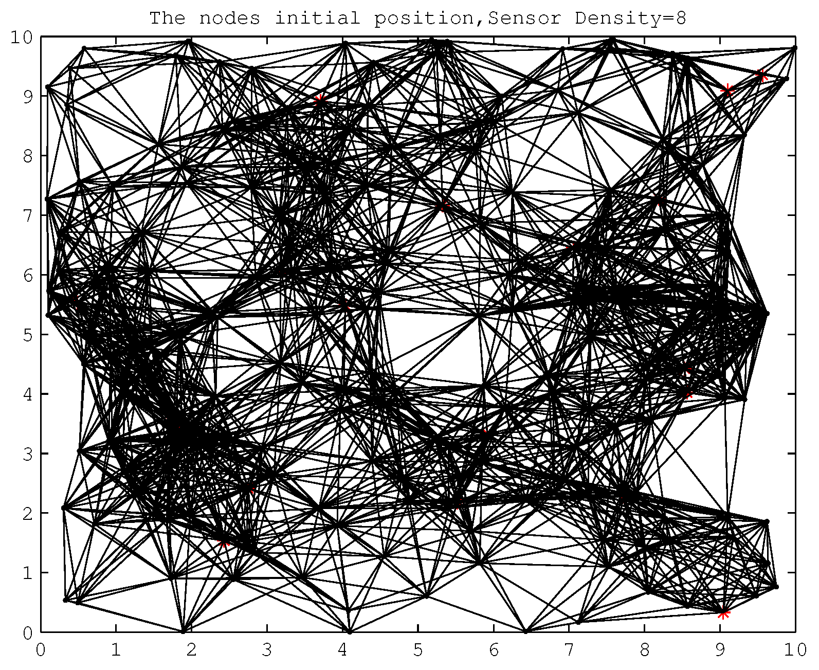
Figure 3.
Irregular Topology: O-shape.
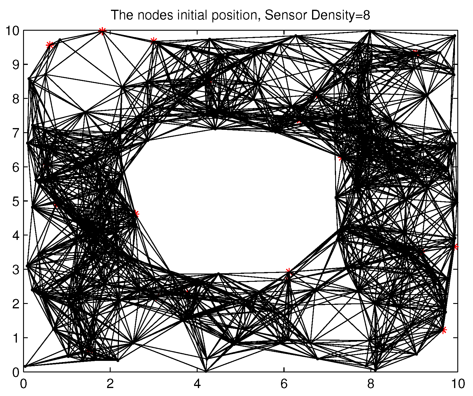
Figure 4.
Irregular Topology: C-shape.
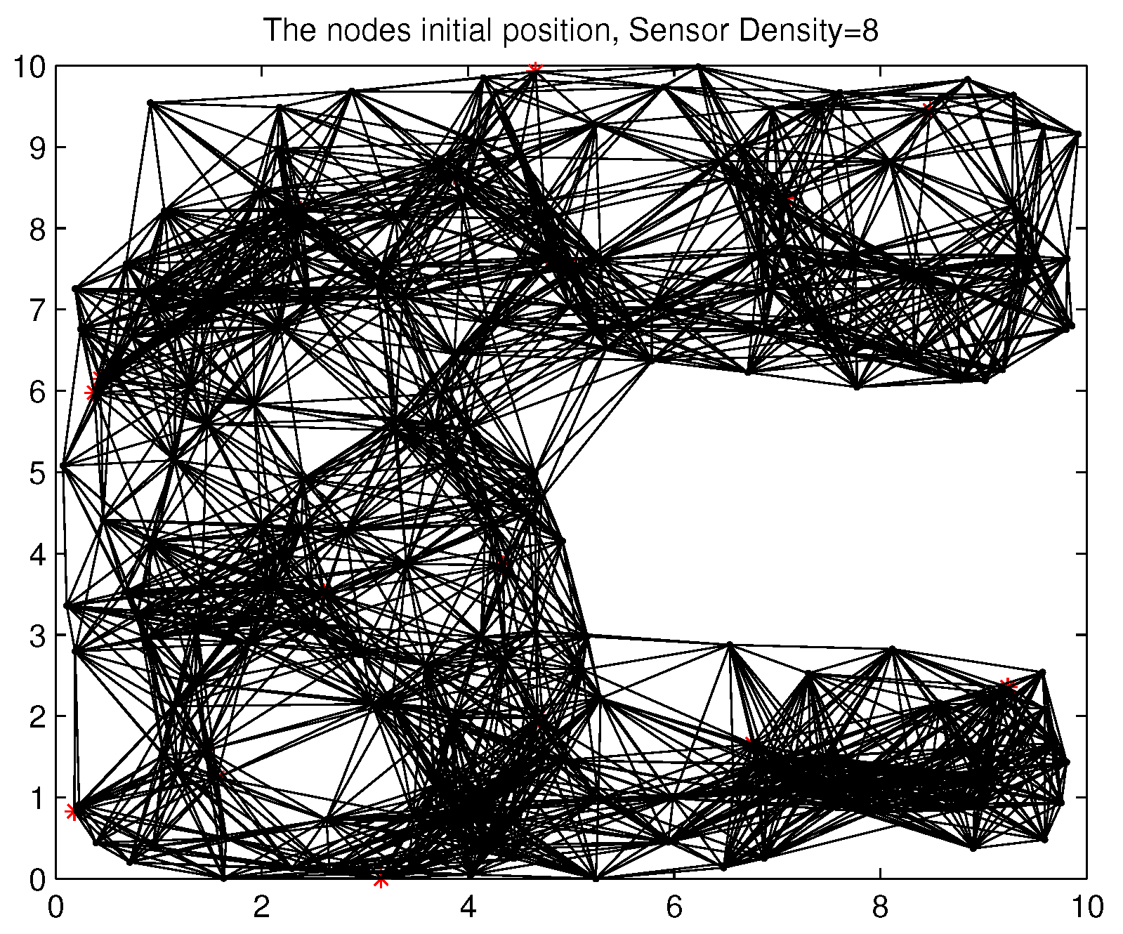
© 2017 by the authors. Licensee MDPI, Basel, Switzerland. This article is an open access article distributed under the terms and conditions of the Creative Commons Attribution (CC BY) license (http://creativecommons.org/licenses/by/4.0/).
Share and Cite
MDPI and ACS Style
Paul, A.K.; Sato, T. Localization in Wireless Sensor Networks: A Survey on Algorithms, Measurement Techniques, Applications and Challenges. J. Sens. Actuator Netw. 2017, 6, 24. https://doi.org/10.3390/jsan6040024
AMA Style
Paul AK, Sato T. Localization in Wireless Sensor Networks: A Survey on Algorithms, Measurement Techniques, Applications and Challenges. Journal of Sensor and Actuator Networks. 2017; 6(4):24. https://doi.org/10.3390/jsan6040024
Chicago/Turabian StylePaul, Anup Kumar, and Takuro Sato. 2017. "Localization in Wireless Sensor Networks: A Survey on Algorithms, Measurement Techniques, Applications and Challenges" Journal of Sensor and Actuator Networks 6, no. 4: 24. https://doi.org/10.3390/jsan6040024
Note that from the first issue of 2016, this journal uses article numbers instead of page numbers. See further details here.