Bayesian-Optimization-Based Peak Searching Algorithm for Clustering in Wireless Sensor Networks

Graduate School of Applied Informatics, University of Hyogo, Computational Science Center Building 5-7F 7-1-28 Minatojima-minamimachi, Chuo-ku Kobe, Hyogo 6570047, Japan
*
Author to whom correspondence should be addressed.
J. Sens. Actuator Netw. 2018, 7(1), 2; https://doi.org/10.3390/jsan7010002
Submission received: 31 October 2017
/
Revised: 25 December 2017
/
Accepted: 29 December 2017
/
Published: 2 January 2018
(This article belongs to the Special Issue Sensors and Actuators in Smart Cities)
Abstract
:We propose a new peak searching algorithm (PSA) that uses Bayesian optimization to find probability peaks in a dataset, thereby increasing the speed and accuracy of clustering algorithms. Wireless sensor networks (WSNs) are becoming increasingly common in a wide variety of applications that analyze and use collected sensing data. Typically, the collected data cannot be directly used in modern data analysis problems that adopt machine learning techniques because such data lacks additional information (such as data labels) specifying its purpose of users. Clustering algorithms that divide the data in a dataset into clusters are often used when additional information is not provided. However, traditional clustering algorithms such as expectation–maximization (EM) and algorithms require massive numbers of iterations to form clusters. Processing speeds are therefore slow, and clustering results become less accurate because of the way such algorithms form clusters. The PSA addresses these problems, and we adapt it for use with the EM and algorithms, creating the modified and algorithms. Our simulation results show that our proposed and algorithms significantly decrease the required number of clustering iterations (by 1.99 to 6.3 times), and produce clustering that, for a synthetic dataset, is 1.69 to 1.71 times more accurate than it is for traditional EM and enhanced (++) algorithms. Moreover, in a simulation of WSN applications aimed at detecting outliers, correctly identified the outliers in a real dataset, decreasing iterations by approximately 1.88 times, and was 1.29 times more accurate than EM at a maximum.
1. Introduction
Over the past decade, wireless sensor networks (WSNs) have been widely applied in applications that involve analyzing collected data to improve quality of life or secure property. For example, sensor nodes are present in homes, vehicle systems, natural environments, and even satellites and outer space. These sensors collect data for many different purposes, such as health monitoring, industrial safety and control, environmental monitoring, and disaster prediction [1,2,3,4]. In such WSN applications, sensing data can be manually or automatically analyzed for specific purposes. However, in the age of big data, an increasing amount of sensing data is required for precise analysis in the WSN applications. Consequently, it is difficult or, in some cases, even impossible to manually analyze all of the collected data.
There are several conventional ways to automatically manage the collected data. The most typical and the easiest method is to set threshold values that correspond to sensing events. Events are triggered once the data exceed these thresholds. However, the thresholds in large-scale WSNs vary, and change due to environment changes. Moreover, precise analysis results cannot be obtained through the use of thresholds alone.
A complementary approach uses supervised machine learning. In this approach, a model is trained that can categorize sensing data into the different states required by an application. However, because sensing data labels are required in the training phase, extra work is required to manage the data. This process is particularly difficult when the dataset is large. Moreover, if the sensing environment changes, certain labels must also change. It is difficult to maintain a functional model under conditions where labels change frequently; this affects the analysis results.
Unsupervised machine learning methods are feasible and well-studied, and are not associated with the data labeling problems described above. Clustering is an important and common method in such approaches. In clustering, the overall features of the dataset are extracted. Then, the data are divided into clusters according to their features. As a result, data labeling is not required, and the data-labeling difficulties that occur in supervised approaches can be avoided. However, in state-of-the-art clustering methods such as the () [5] and k-means [6] algorithms, a massive number of iterations must be performed in order to form clusters, and a significant amount of computation time is required. Furthermore, because these algorithms use random starting data points as initial center points to form clusters, and because the number of clusters is not precisely determined, the clustering results become less accurate. To address these problems, in this paper, we propose a peak searching algorithm () for improving clustering algorithm capabilities.
Our approach should be applicable to different dataset distributions. Therefore, the collected sensing dataset is considered to be generated by a Gaussian mixture model composed of several different Gaussian distributions. If the number of Gaussian distributions and appropriate initial center points are known, clustering algorithms can appropriately divide the dataset into different clusters because each Gaussian distribution corresponds to a cluster. The proposed employs a Bayesian optimization (BO) strategy that uses a Gaussian process [7]. Bayesian optimization is typically used for hyper-parameter optimizations; to the best of our knowledge, our approach is the first to use BO to improve clustering. Moreover, other Bayesian theorem based algorithms, such as [8,9,10,11], are also appropriate optimization strategies for training online and offline machine learning algorithms.
Given a collected dataset, the searches for the data points with the highest probability values (i.e., peaks in the dataset). A Gaussian distribution peak is a point that corresponds to the mean. By searching the peaks, we can obtain appropriate initial center points of Gaussian distributions, hence, the corresponding clusters. This method overcomes the difficulties associated with the hard determination of starting data points in traditional cluster algorithms, thereby reducing the number of iterations. By using the , cluster algorithms can form clusters using peak points instead of random starting points, which improves the clustering accuracy.
We used simulations to investigate the potential of the proposed for improving algorithm performance. To measure performance improvements, we applied the to the and algorithms. We refer to these modified algorithms as and , respectively. The simulation results showed that, for and , the required numbers of clustering iterations were significantly reduced by to times. Additionally, for synthetic datasets, clustering accuracy was improved by to times relative to the traditional and enhanced version of , i.e., ++ [12].
The proposed method can accurately group data into clusters. Therefore, any outliers in a dataset can be clustered together, making them possible to identify. Because outliers obviously reduce the capabilities of the WSN applications, we also conducted a simulation using a real WSN dataset from the Intel Berkeley Research lab (Berkeley, CA , USA). This allowed us to compare the outlier-detection capabilities of and . Our simulation results showed that correctly identified outliers, decreased iterations by approximately times, and improved accuracy by times at a maximum.
The remainder of this paper is organized as follows. Section 2 outlines related works, while Section 3 introduces BO. Section 4 describes the proposed and Section 5 presents the simulation results. Section 6 presents a discussion of this work. Section 7 summarizes key findings, presents conclusions, and describes potential future work.
2. Related Works
This section describes the techniques used in the clustering algorithms, which are used to automatically divide a collected dataset into different clusters. There are two main types of clustering approaches. The first is based on parametric techniques. To cluster a dataset, the parameters of the statistical model for a dataset must be calculated. The algorithm is a parametric technique. The second type of clustering approach uses non-parametric techniques, in which the calculated parameters of a statistical model are not required for clustering a dataset. and ++ are non-parametric techniques.
We describe the two clustering approaches in the following subsections. Moreover, because outlier detection is critical in the WSN applications, we describe some relevant outlier detection approaches.
2.1. Parametric Techniques
Parametric techniques assume that a dataset is generated from several parametric models, such as Gaussian mixture models. The clustering process is conducted by calculating the parameters of each Gaussian model, and assuming that data points in the same cluster can be represented by the same Gaussian model. Usually, a Gaussian model is chosen as the default model because it conforms to the central limit theorem [13,14] parametric techniques used. From the collected dataset, they calculated detailed a priori estimates of statistical parameters for the assumed statistical model (for example, the mean, median, and variance). This allowed them to fit statistical models.
EM [5] is a famous and widely used algorithm for clustering datasets using parametric techniques. The algorithm first calculates responsibilities with respect to given parameters (means and variances). This is referred to as the E-step. Then, the algorithm uses the responsibilities to update the given parameters. This is referred to as the M-step. These two steps are iteratively executed until the parameters approach the true parameters of the dataset. When those parameters are determined, the Gaussian models in the Gaussian mixture model are fixed. Therefore, clustering can be accomplished using the Gaussian models.
There are many benefits associated with parametric techniques: (i) such techniques assign a probability criterion to every data point to determine whether or not it belongs to a cluster; and (ii) such techniques do not require additional information (for example, labels on data points that indicate their statuses). On the other hand, parametric techniques cannot be deployed in a distributed way because a significant number of data points are required to estimate the mean and variance. Thus, methods that use parametric techniques are deployed in a centralized way.
2.2. Non-Parametric Techniques
Some algorithms use non-parametric techniques, which cluster datasets without using statistical models. Non-parametric techniques make certain assumptions, such as density smoothness. Typical methods use histograms, as in [15,16,17]. Histogram-based approaches are appropriate for datasets in low-dimensional spaces because the calculations in histogram-based techniques have an exponential relationship with the dimensions of a dataset. Therefore, this type of approach has low scalability to problems with larger numbers of data points and higher-dimensional spaces.
One typical non-parametric cluster algorithm is k-means [6]. In k-means, when candidate cluster centers are first provided to the algorithm, the number of centers is equal to the number of clusters. Then, is used to calculate the sum of the distances from the center of each cluster to every data point. These two steps are iteratively executed, and updates the given cluster centers by minimizing the calculated sum. When cluster centers are determined, clusters are formed. However, cannot guarantee that the candidate centers will be close to the true cluster centers. The iterations and clustering accuracy of the algorithm are not satisfying.
To overcome the disadvantages of , Arthur and Vassilvitskii [12] proposed ++, which is based on the algorithm. ++ and are different because ++ uses the number of k values to execute a calculation that identifies the appropriate data points to use as the initial centers. In contrast, in the algorithm, the initial centers are randomly selected, which increases the number of clustering iterations. Therefore, ++ requires fewer iterations than .
In conclusion, there are disadvantages associated with the use of both parametric and non-parametric techniques in the WSNs. Parametric techniques can only estimate a model when sufficient data is available, and they are therefore difficult to use in a distributed way. While non-parametric techniques can be executed in a distributed way in the WSNs, they cannot provide a probability criterion for detection. Moreover, both techniques require a massive number of iterations to form clusters and use random starting data points. These require significant computing power and have low accuracy.
2.3. Outlier Detection in WSN Applications
Outliers are very common in collected datasets for two reasons. First, sensor nodes are vulnerable to failure because the WSNs are often deployed in harsh environments [18,19,20,21]. Outliers are commonly found in datasets collected by the WSNs installed in harsh environments [22,23]. Second, noise in wireless signals and malicious attacks both create outliers [24,25], which obviously reduce the WSN capabilities.
The clustering methods are also used for outlier detection in the WSN applications. For instance, to robustly estimate the positions of sensor nodes, Reference [26] used the algorithm to iteratively detect outlier measurements. The algorithm was used to calculate variables that could indicate whether or not a particular measurement was an outlier. Reference [27] conducted similar work using algorithms to detect outliers. Additionally, Reference [28] proposed a novel flow-based outlier detection scheme based on the clustering algorithm. This method separated a dataset containing unlabeled flow records into normal and anomalous clusters. Similar research by [29] used to detect heart disease. However, approaches using and to detect outliers suffer from the previously mentioned problems of clustering iteration and accuracy. The approach that we introduce later in this paper can solve such problems.
3. Bayesian Optimization
Before a dataset can be divided into clusters, the starting data points of clusters in the dataset must be determined. In particular, the number of peak points (a peak point is a data point corresponding to the maximum probability) in a dataset corresponds to the number of clusters. In this study, we use BO to identify peak points. Typically, we do not know the form of the probability density function . Nevertheless, we can obtain the approximate value of at data point , with some noise. For example, we can approximately compute the density of a certain volume. This density is an approximate value of the probability density (see Section 4). However, obtaining the maximum density can be computationally expensive because of the large number of data points. To reduce computation costs, we used BO [30,31], a very powerful strategy that fully utilizes prior experience to obtain the maximum posterior experience at each step. This allows the maximum density to be approached. Thus, fewer data points are required to obtain the maximum density. In the following subsection, we introduce the Gaussian process used in BO.
3.1. Gaussian Process
In BO, a Gaussian process (GP) is used to build a Gaussian model from the provided information. The model is then updated with each new data point. Assume that a set of data points contains t elements: . We use the notation to represent the set of data points. Each of these points exists in a space. An example data point is .
There is an intuitive analogy between a Gaussian distribution and a GP. A Gaussian distribution is a distribution over a random variable. In contrast, the random variables of a GP are functions. The mean and covariance are both functions. Hence, function follows a GP and is defined as follows:
where is the mean function, and is the kernel function of the covariance function.
Suppose that we have a set of data points and their corresponding approximate probability density . We assume that function can map a data point to its probability density with some noise. For concision, we will use to represent the set of functions for each data point . For the collected dataset, is the given information. For convenience, we assume that follows the GP model, which is given by an isotropic Gaussian whose initial mean function is zero and covariance function is calculated using , as follows: ( consists of the kernel functions)
Once, we have calculated , we build a GP model from the information provided.
A new data point also follows . According to the GP properties, and are jointly Gaussian:
where
Moreover, we want to predict the approximate probability density of the new data point . Using Bayes’ theorem and , we can obtain an expression for the prediction:
where
We can observe that and are independent of and that we can calculate using the given information.
3.2. Acquisition Functions for Bayesian Optimization
Above, we briefly describe how to use the given information to fit a GP and update the GP by incorporating a new data point. At this point, we must select an appropriate new data point to use to update the GP, so that we can obtain the maximum value of . To achieve this, we could use BO to realize exploitation and exploration. Here, exploitation means that we should use the data point with the maximum mean in the GP because that point fully uses the given information. However, this point cannot provide additional information about the unknown space. Exploration means that a point with a larger variance in the GP can provide additional information about the unknown area. The acquisition functions used to find an appropriate data point are designed on the basis of exploitation and exploration. There are three popular acquisition functions: probability of improvement, expectation of improvement, and upper confidence bound criterion.
The probability of improvement (PI) function is designed to maximize the probability of improvement over , where . The resulting cumulated distribution function is:
where is the exploration strength, which is provided by the user.
The expectation of improvement (EI) is designed to account for not only the probability of improvement, but also the potential magnitude of improvement that could be yielded by a point. The EI is expressed as
The upper confidence bound (UCB) criterion uses the confidence bound, which is the area representing the uncertainty between the mean function and variance function in Equation (3). The UCB is compared with the other two acquisition functions, and is relatively simple and intuitive. In detail, it directly uses the mean and variance functions obtained from the given information. A potential new data point is presented by the sum of (i) the mean function, and () a constant times the variance function. That is, given several potential new data points, the data point with the largest UCB will be selected as the next new data point. Moreover, , which is greater than 0, indicates how many explorations are expected. The UCB formula is
These three acquisition functions are suited to different datasets, and allow us to obtain an appropriate new data point. The BO algorithm (Algorithm 1) is shown below.
| Algorithm 1: BO |
 |
4. Peak Searching Algorithm
In this section, we first introduce some preliminary information related to our proposed algorithm. Then, we explain the algorithm.
4.1. Preliminary Investigations
In most cases, the environment can be represented as a collection of statuses that indicate whether or not certain events have occurred. Such events include fires, earthquakes, and invasions. The data points collected by the sensor nodes contain measurements that describe the statuses of these events. One can assume that the collected dataset is generated by a Gaussian mixture model (GMM) because the data points contained in the dataset are collected from the normal environment, or from natural events. Thus, before fitting a GMM, it is necessary to clarify the peaks of the GMM because each peak is a point that has the largest probability corresponding to a Gaussian distribution. Therefore, we need to know the probability of each data point when we search for the dataset peaks. Although the probability density function is unknown, it can be approximated using alternative methods, which are shown as follows.
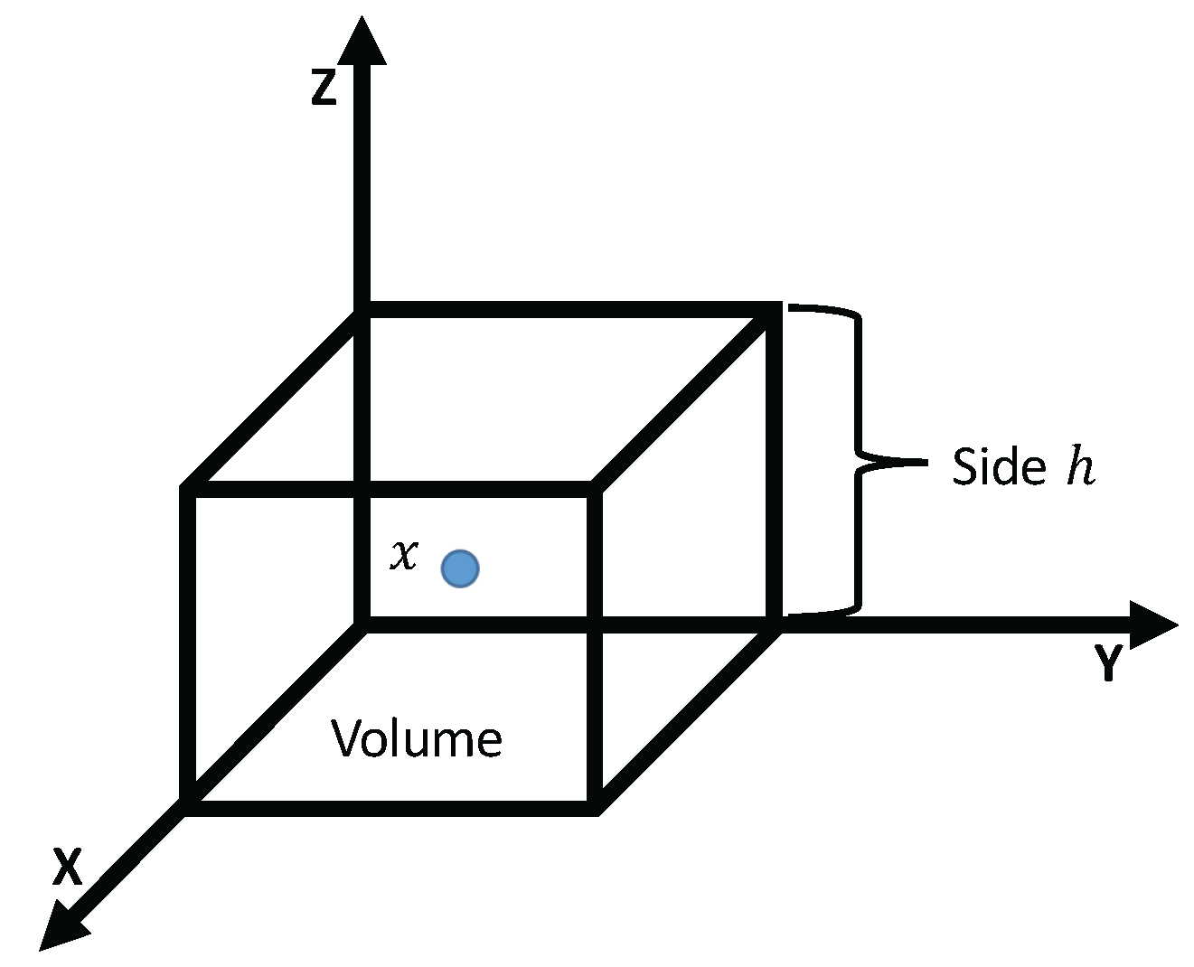
One type of method assumes that the set of data points exists in a space. The probability of data point can then be approximated as follows: set as the center of a volume with side h. Figure 1 shows an example of a volume in 3D space, where the length of each side is h; and the density of the volume with center , calculated using Equation (8) [31], is approximately equal to the probability at data point . The density in this formula depends on the length of side h in the volume and the number T (that is, the number of neighbors of data point in the volume). N is the total number of data points in the dataset and is the size of the volume. Thus, to search for the peaks, we must calculate the densities of all of the different data points using Equation (8). However, this is computationally expensive:
Another method fixes h and applies a kernel density estimator [31]. In this case, the probability of data point can be calculated as
where is the kernel function and T is the number of data points in a volume with side h. Then, the largest value of occurs along the gradient of Equation (9), which is
By setting Equation (10) equal to zero, we can calculate the point along the gradient that has the largest . With this method, we do not need to search through the unimportant data points, which reduces the time required to identify peaks. However, Equations (9) and (10) are difficult to solve. Moreover, the length of side h affects the peak search results. Firstly, it supposes that all of the volumes have the same size because they have the same h. Secondly, an inappropriate h value will lead to an incorrect result. In particular, h values that are too large cause over-smoothing in high-density areas, while h values that are too small cause significant noise in low-density areas. To overcome these shortcomings, we introduce the , which we describe in the following subsection.
4.2. The Algorithm
We propose a peak searching algorithm () that does not consider parameter h. We will use simulations to investigate the details of the , which can be used to improve the speed and accuracy of clustering algorithms such as and .
In Equation (10), is a vector that starts at point and ends at neighboring point . Because a kernel function is used to calculate the inner product of the vector, in this case, the inner product is equal to the vector mode. Moreover, it calculates the largest and the location of data point where on the vector at times the mode of the vector. Therefore, the largest probability for finding the peak lays on this vector. This allows us to concentrate only on the vector, without considering constants and h. Hence, we propose using to represent the vector in the as
In Equation (11), only is searched. A significant amount of non-important space is not searched. However, many probabilities must be calculated along . Moreover, because there are too many data points on the vector , it becomes impossible to search for the best data point with the largest probability in a limited amount of time. Hence, we apply BO when searching for the largest probability along . BO optimizes the method for searching the maximum probability value mentioned in Algorithm 1. However, as we mentioned in Section 3, the form of probability function is not known, and it can instead be represented by an approximate probability function, which is in Algorithm 1 line 4. Therefore, in this paper, we use Equation (8) to calculate the approximate probability function, which we use in the proposed algorithm. Equation (8) is simpler and more practical for finding dataset peaks. The following describes the details of the proposed .
Next, we will explain how the works in accordance with Algorithm 2. The initializing step requires a number of starting data points from which to begin the search for peaksbecause the dataset may contain multiple peaks. Therefore, the randomly selects M starting points, . For convenience, we will use starting point to describe the details of the method. Vector is calculated using Equation (11) in line 1. The peak searching process shown in Figure 2 contains four steps. In Step 1, the uses Algorithm 1 to search for the peak. That is, data point , which has a maximum probability along . The probability denoted by is calculated using Equation (8) as shown in line 4. In Step 2 in line 5, a new vector is calculated on the basis of and its T neighboring data points. In Step 3, the method searches for the peak along in line 6. Notice that data points and are possible dataset peaks. Step 4 starts from line 7 to 14, and the method repeats these steps until the difference between and gets close enough to zero. At this point, data point is selected as a dataset peak. The same four steps are used with the other starting data points to identify all peaks in the dataset.
| Algorithm 2: PSA |
 |
5. Simulation and Analysis
In this section, we investigate the efficiency of the proposed . Because the is a method for improving clustering algorithms, we must use it in state-of-the-art clustering algorithms to evaluate the extent to which the can improve those algorithms. As mentioned in Section 2, and are common clustering algorithms. Here, variations of those algorithms using the are referred to as and , respectively. In and , the first searches the peaks of the collected dataset. Then, and use the obtained peaks as the initial starting points to start clustering. In the simulations, we assume that the collected datasets follow GMMs, and that the number of peaks found by the is equal to the number of Gaussian distributions.
We conducted simulations using synthetic datasets and a real dataset. In simulations with synthetic datasets, we compared the accuracies and iterations of and with those of the original (), , and ++ algorithms. Moreover, because recall and precision are important evaluation indicators, we also used the simulations to compare recalls and precisions. In the simulation using a real dataset, we simulated our methods in order to detect outliers. Because a real dataset could be either isotropic or anisotropic, and because has a weak effect on anisotropic datasets, we only compared to for the real dataset.
5.1. Simulation on Synthetic Datasets
5.1.1. Synthetic Dataset
We generated two synthetic datasets, whose data points contained two features. Each dataset was generated using a GMM that contained two different Gaussian distributions. The Gaussian distributions in the first dataset were isotopically distributed; their true peaks (means) were and and their variances were and , respectively. The Gaussian distributions in the second synthetic dataset were transformed using the following matrix to create anisotropically distributed datasets:
The two synthetic datasets are shown in Figure 3. The two synthetic datasets are appropriate for these types of simulations because they can represent both easy and difficult clustering situations. This allows us to evaluate the effects of our algorithm.
5.1.2. Simulations and Results
To estimate the extent to which the can improve clustering capabilities, we compared with the original () algorithm. Both and use to fit a GMM, and have a time complexity of , where N is the number of data points. Hence, we cannot use time complexity to compare and . Computational efficiency can also be measured from the number of iterations. The algorithm contains two steps: the E-step and the M-step. These two steps are iteratively executed to fit a GMM, and are the core calculations of this algorithm. Hence, we compared the number of iterations in (i.e., how many E-steps and M-steps were executed) with the number of iterations in . Note that the algorithm does not use , so its calculations start at randomly selected initial starting points.
and were executed 200 times for the two different datasets. Figure 3 shows 200 peak searching results for . The dark crosses indicate the peaks identified by . We can see that, in the isotropically distributed dataset, the identified peaks are very close to the true peaks. In the anisotropically distributed dataset, the identified peaks are also close to the true peaks. Figure 4 illustrates the number of iterations (y-axis) for each size of dataset (x-axis). In the peak searching step, three different acquisition functions are used (, , and ), and their calculation efficiencies are compared. According to the results shown in Figure 4, there were to times fewer iterations for than . In other words, the improved the calculation efficiency of by to . Moreover, we can see that there is no obvious difference between the three acquisition functions.
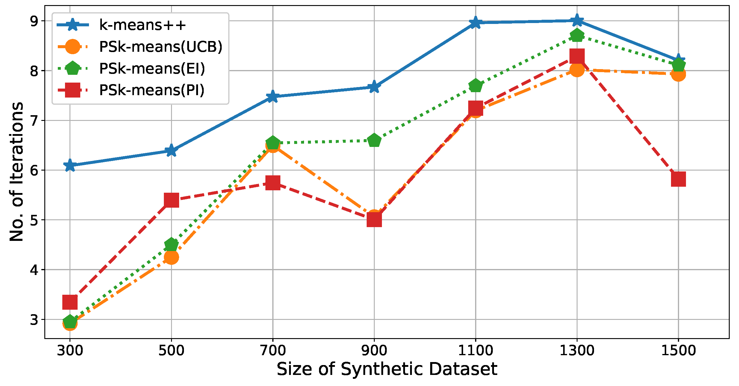
Because we wanted to fairly estimate the extent to which the proposed improves clustering capabilities, we compared the to ++ in another simulation. ++ uses a special method to calculate its initial points, and its clustering method increases the speed of convergence. Note that both and ++ are based on , which has a time complexity , where N is the number of data points and T is the number of iterations. Similarly, we cannot use time complexity to compare calculation efficiencies. However, we can compare the number of iterations required for to that required for ++. Both of these algorithms were executed 200 times with the two different datasets, and the results are shown in Figure 5.
The simulation results are shown in Figure 5. The average number of iterations for is reduced by to times compared with the number of iterations for ++. In other words, the improved the calculation efficiency of by to . Additionally, there was no obvious difference between the three acquisition functions.
5.1.3. Performance Estimation of Clustering
, , and are three commonly used measurements for estimating machine learning algorithm performance. Therefore, we adopt these measurements to quantify the performances of our proposed algorithm. In simulations, a dataset containing two clusters is generated by GMM. To explain these measurements, we assume that the two clusters are cluster A and cluster B. Data points belonging to cluster A are considered to be positive instances, while those that belong to cluster B are considered to be negative instances. If a data point from cluster A is correctly clustered into cluster A, it is a true positive (TP) result. Otherwise, it is a false positive result (FP). Similarly, if a data point from cluster B is correctly clustered into cluster B, that is a true negative (TN); otherwise, it is a false negative (FN). Overall can be calculated as follows:
is equal to the ratio of TP to the total number of positive instances. It is based on the total positive instances, and shows how many positive instances can be detected by the algorithm. It is calculated as
From a prediction standpoint, indicates how many TPs occur in the detected positive instances. It presents the proportion of TP to the total number of data points that are detected as positive, which is equal to TP + FP. is calculated as
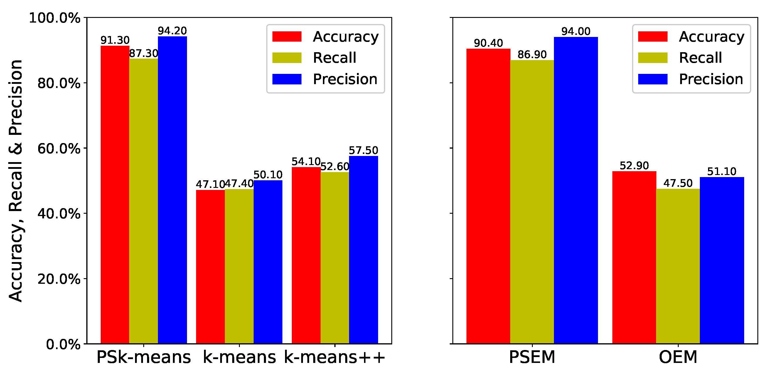
We estimated the , , and of the and clustering algorithms, and compared the values with those for , ++, and . We repeated this estimation 200 times for each dataset; the average accuracy of each algorithm is shown in Figure 6 and Figure 7. The isotropic datasets shown in Figure 3 are difficult to cluster because the two clusters partially overlap and their centers are very close together. We can see from the simulation results shown in Figure 6 that the estimations of , ++, and are similar. However, and show a great improvement over their original algorithms. The accuracy of is times higher than that of ++, while that of is times higher than that of . The recall of is times higher than that of ++, and the recall of is times higher than that of . Moreover, the precision of is times higher than that of ++’s. The precision of is times higher than that of .
The results for the anisotropic datasets are shown in Figure 7. Because the anisotropic datasets are elliptical, as shown in Figure 3, and the two datasets are very close together, the datasets are very difficult to cluster. As a result, and ++ exhibit low estimation performance, and yields little improvement. However, the accuracy of was times higher than that of , and its recall and precision were and times higher, respectively, than they were for . Accordingly, we can see that the can improve clustering accuracy.
5.2. Simulation on a Real Dataset from Intel Berkeley Research Laboratory
We used a real sensor dataset from the Intel Berkeley Research Laboratory [32] to assess outlier detection performance. In the simulation, we only considered two features for each data point: temperature and humidity. Each sensor node contained 5000 data points, which are shown in Figure 8.
Because the original dataset did not provide any outlier information or labels, we manually cleaned the data by removing values that fell outside a normal data range. All of the remaining data points were considered to be normal. Table 1 lists the normal data ranges.
After completing this step, a uniform distribution was used to generate artificial outliers. Temperature outliers were generated within a range of (27–30) C, and humidity outliers were generated within a range of (42–46)%. Thus, some outliers can fall inside the normal range with the same probability. Outliers were then inserted into the normal dataset. We produced four different cases, in which the outliers accounted for , , , and of the total normal data points.
5.2.1. Setting of WSNs
and were run for a real dataset from the Intel Berkeley Research Laboratory. The deployment of the WSNs is shown in Figure 9. There were 54 sensor nodes, each of which had a sensor for collecting humidity, temperature, light, and voltage values. Temperatures were provided in degrees Celsius. Humidity was provided as temperature-corrected relative humidity, and ranged from . Light was expressed in Lux (1 Lux corresponds to moonlight, 400 Lux to a bright office, and Lux to full sunlight), and voltage was expressed in volts, ranging from . The batteries were lithium ion cells, which maintain a fairly constant voltage over their lifetime; note that variations in voltage are highly correlated with temperature. We selected data from 10 sensor nodes (nodes 1 to 10) to test our method, and used only humidity and temperature values.
In this simulation, we assumed that the WSN was hierarchical and consisted of classes. (“Cluster” is used in the WSNs to describe a group of sensor nodes. However, “cluster” can also refer to a group of similar data points in data mining. In this paper, we use “class” instead of cluster to describe a group of sensor nodes). Each class contained one class head (CH) and other member sensor nodes (MSNs). The MSNs sent the data points collected over a certain time period to the CH, which used the proposed method to monitor whether the dataset collected from its members contained outliers. The configuration of the WSNs is shown in Figure 10.
5.2.2. Results
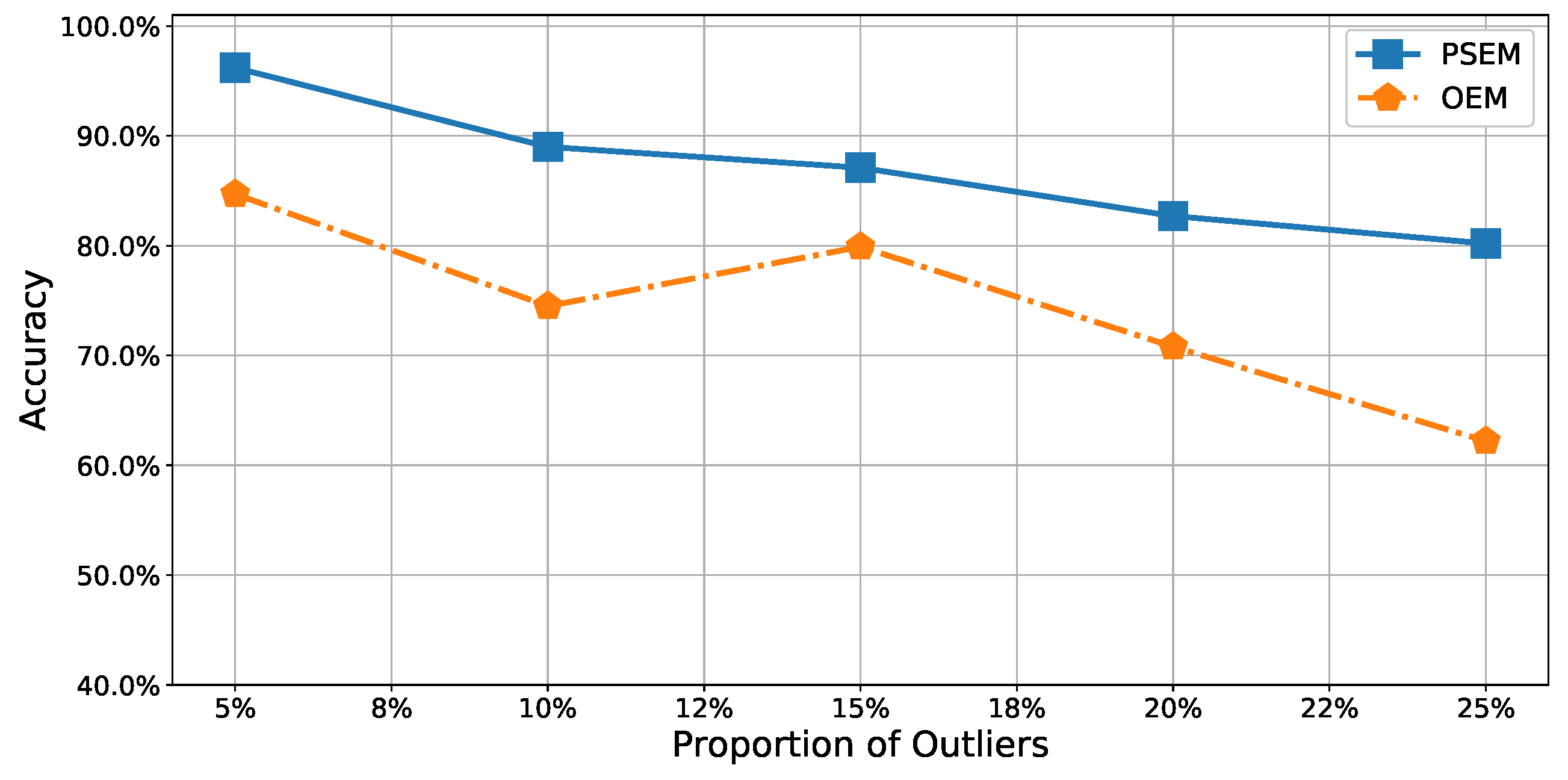
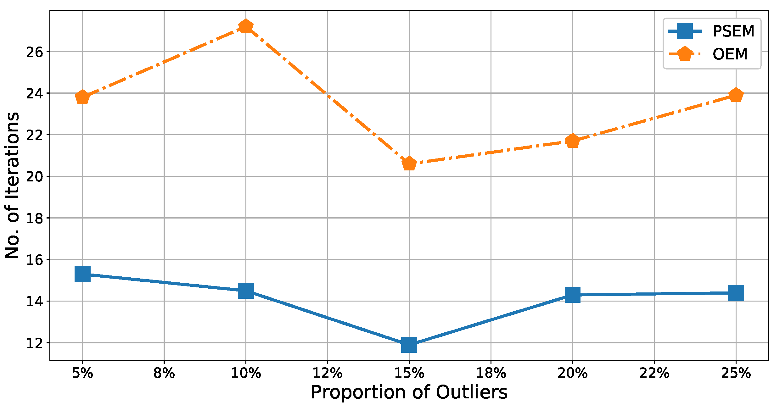
Using the real dataset, we tested the proposed and compared it with the . The CH executed the or to detect outliers, and sent outlier reports to the base station. We generated four different datasets, containing , , , and outliers. (Figure 11 and Figure 12).
It was relatively easy to detect outliers in the test dataset containing only outliers because the proportion of outliers was so low. Thus, the accuracy of our method approached for outliers. In contrast, the accuracy of the was only approximately . In the other datasets, more outliers fell within the normal dataset. In such cases, it was difficult to detect the outliers; the accuracies of both methods decreased as the proportion of outliers increased. However, remained more accurate than . In the worst case, with outliers in the test dataset, its accuracy of was approximately , while the accuracy of was only approximately . That is, was about to times more accurate than . Moreover, Figure 12 shows the number of iterations was to times lower for , meaning that improved the calculation efficiency of by to . Because accuracy and iteration numbers are very important metrics for assessing the clustering algorithm efficiency, this simulation result demonstrated the practical significance of , and, therefore, of the .
6. Discussion
In this section, we describe other important aspects of the WSNs, such as WSN power consumptions and lifetime. We also discuss the advantages and disadvantages of the proposed method.
Because most sensor nodes in the WSNs are powered by batteries, sensor node power consumptions, WSN lifetime, and energy efficiency are also important problems affecting the quality of a WSN. Mostafaei et al. [33] proposed an algorithm PCLA to schedule sensors into active or sleep states, utilizing learning automata to extend network lifetime. Our previous work attempted to extend battery life by reducing peak power consumption. We scheduled sensor execution times [34], and used optimized wireless communication routes to reduce energy consumption, with the goal of prolonging network lifetimes [35,36]. If the proposed can be applied in such approaches to analyze data using clustering methods, then energy consumption can be further reduced. Because the can reduce clustering iterations, the required computational power decreases, leading to energy savings.
The proposed algorithm has advantages and disadvantages. In conventional clustering methods such as and , cluster-forming procedures are started at random data points. There are two disadvantages associated with this. First, correct clusters may not be able to form from random starting points. Second, because random staring points may not occur near cluster centers, massive iterations may be needed to update random points to approach the cluster centers. However, because the can identify the peak points near cluster centers, it is a better approach for forming clusters than an algorithm starting from a random point. Therefore, clustering algorithms using the can form clusters more accurately. Moreover, using peak points as the starting points to form clusters can significantly reduce clustering iterations because peak points are the desired points.
There are some disadvantages associated with the . The use BO and are, therefore, affected by the problems associated with BO. A particular issue is that a priori design is critical to efficient BO. As mentioned in Section 3, BO uses GPs to build Gaussian models with Gaussian distributions, making the resulting datasets transcendental. If a dataset does not have a Gaussian distribution, the may be less efficient. Another weak point of the is that it is centralized. It is not suited for highly distributed WSNs where data analyses are conducted at each sensor node.
7. Conclusions
In this paper, we proposed a new for improving the performance of clustering algorithms (i.e., for improving accuracy and reducing clustering iterations). BO is used to search for the peaks of a collected dataset in the . To investigate the efficiency of the , we used the to modify and algorithms. The new algorithms were named and , respectively.
Using simulations, we investigated the performance of and relative to that of and ++. We conducted simulations using both synthetic datasets and a real dataset. For synthetic datasets, and reduced iterations by approximately and times, respectively, at a maximum. Moreover, they improved clustering accuracy by times and times, respectively, at a maximum. On a real dataset for outliers’ detection purpose, reduced iterations about times, and improved clustering accuracy by times at a maximum. These results show that our proposed algorithm significantly improves performance. We obtained the same conclusions by illustrating the recall and precision improvements for and .
In the future, we will improve this method so that it can be used with high-dimensional data, such as images collected by a camera. Moreover, we would like to deploy the peak searching algorithm with sensor nodes, in order to allow CHs to obtain peak searching results from their neighbors; this will reduce the calculation time required for the peak search. Thus, clustering can be implemented in the sensor node and communication costs can be reduced.
Acknowledgments
This work was supported by the Japan Society for the Promotion of Science (JSPS KAKENHI Grant Numbers 16H02800, 17K00105, and 17H00762).
Author Contributions
Tianyu Zhang, Qian Zhao, and Kilho Shin conceived and designed the algorithm and experiments. Tianyu Zhang performed the experiments, analyzed the data, and was the primary author of this paper. Yukikazu Nakamoto gave advice on this work and helped revise the paper. Additionally, Qian Zhao and Kilho Shin helped revise the paper.
Conflicts of Interest
The authors declare no conflict of interest.
References
- Sung, W.T. Multi-sensors data fusion system for wireless sensors networks of factory monitoring via BPN technology. Expert Syst. Appl. 2010, 37, 2124–2131. [Google Scholar] [CrossRef]
- Hackmann, G.; Guo, W.; Yan, G.; Sun, Z.; Lu, C.; Dyke, S. Cyber-physical codesign of distributed structural health monitoring with wireless sensor networks. IEEE Trans. Parallel Distrib. Syst. 2014, 25, 63–72. [Google Scholar] [CrossRef]
- Oliveira, L.M.; Rodrigues, J.J. Wireless Sensor Networks: A Survey on Environmental Monitoring. J. Clin. Microbiol. 2011, 6, 143–151. [Google Scholar] [CrossRef]
- Wu, C.I.; Kung, H.Y.; Chen, C.H.; Kuo, L.C. An intelligent slope disaster prediction and monitoring system based on WSN and ANP. Expert Syst. Appl. 2014, 41, 4554–4562. [Google Scholar] [CrossRef]
- Dempster, A.P.; Laird, N.M.; Rubin, D.B. Maximum likelihood from incomplete data via the EM algorithm. J. R. Stat. Soc. Ser. B 1977, 39, 1–38. [Google Scholar]
- Huang, Z. Extensions to the k-means algorithm for clustering large data sets with categorical values. Data Min. Knowl. Discov. 1998, 2, 283–304. [Google Scholar] [CrossRef]
- Rasmussen, C.E.; Williams, C.K. Gaussian Processes for Machine Learning; MIT Press: Cambridge, MA, USA, 2006; Volume 1. [Google Scholar]
- Papaioannou, I.; Papadimitriou, C.; Straub, D. Sequential importance sampling for structural reliability analysis. Struct. Saf. 2016, 62, 66–75. [Google Scholar] [CrossRef]
- Behmanesh, I.; Moaveni, B.; Lombaert, G.; Papadimitriou, C. Hierarchical Bayesian model updating for structural identification. Mech. Syst. Signal Proc. 2015, 64, 360–376. [Google Scholar] [CrossRef]
- Azam, S.E.; Bagherinia, M.; Mariani, S. Stochastic system identification via particle and sigma-point Kalman filtering. Sci. Iran. 2012, 19, 982–991. [Google Scholar] [CrossRef]
- Azam, S.E.; Mariani, S. Dual estimation of partially observed nonlinear structural systems: A particle filter approach. Mech. Res. Commun. 2012, 46, 54–61. [Google Scholar] [CrossRef]
- Arthur, D.; Vassilvitskii, S. k-means++: The advantages of careful seeding. In Proceedings of the Eighteenth Annual ACM-SIAM Symposium on Discrete Algorithms, Society for Industrial and Applied Mathematics, Orleans, LA, USA, 7–9 January 2007; pp. 1027–1035. [Google Scholar]
- Wu, W.; Cheng, X.; Ding, M.; Xing, K.; Liu, F.; Deng, P. Localized outlying and boundary data detection in sensor networks. IEEE Trans. Knowl. Data Eng. 2007, 19, 1145–1157. [Google Scholar] [CrossRef]
- Breunig, M.M.; Kriegel, H.P.; Ng, R.T.; Sander, J. LOF: Identifying density-based local outliers. In Proceedings of the 2000 ACM SIGMOD International Conference on Management of Data, Dallas, TX, USA, 15–18 May 2000; Volume 29, pp. 93–104. [Google Scholar]
- Sheela, B.V.; Dasarathy, B.V. OPAL: A new algorithm for optimal partitioning and learning in non parametric unsupervised environments. Int. J. Parallel Program. 1979, 8, 239–253. [Google Scholar] [CrossRef]
- Eskin, E. Anomaly detection over noisy data using learned probability distributions. In Proceedings of the International Conference on Machine Learning, Citeseer, Stanford, CA, USA, 29 June–2 July 2000. [Google Scholar]
- Eskinand, E.; Stolfo, S. Modeling system call for intrusion detection using dynamic window sizes. In Proceedings of the DARPA Information Survivability Conference and Exposition, Anaheim, CA, USA, 12–14 June 2001. [Google Scholar]
- Dereszynski, E.W.; Dietterich, T.G. Spatiotemporal models for data-anomaly detection in dynamic environmental monitoring campaigns. ACM Trans. Sens. Netw. (TOSN) 2011, 8, 3. [Google Scholar] [CrossRef]
- Bahrepour, M.; van der Zwaag, B.J.; Meratnia, N.; Havinga, P. Fire data analysis and feature reduction using computational intelligence methods. In Advances in Intelligent Decision Technologies; Springer: Berlin/Heidelberg, Germany, 2010; pp. 289–298. [Google Scholar]
- Phua, C.; Lee, V.; Smith, K.; Gayler, R. A comprehensive survey of data mining-based fraud detection research. arXiv. 2010. Available online: https://arxiv.org/ftp/arxiv/papers/1009/1009.6119.pdf (accessed on 29 July 2017).
- Aqeel-ur-Rehman; Abbasi, A.Z.; Islam, N.; Shaikh, Z.A. A review of wireless sensors and networks’ applications in agriculture. Comput. Stand. Interfaces 2014, 36, 263–270. [Google Scholar] [CrossRef]
- Misra, P.; Kanhere, S.; Ostry, D. Safety assurance and rescue communication systems in high-stress environments: A mining case study. IEEE Commun. Mag. 2010, 48, 11206229. [Google Scholar] [CrossRef]
- García-Hernández, C.F.; Ibarguengoytia-Gonzalez, P.H.; García-Hernández, J.; Pérez-Díaz, J.A. Wireless sensor networks and applications: A survey. Int. J. Comput. Sci. Netw. Secur. 2007, 7, 264–273. [Google Scholar]
- John, G.H. Robust Decision Trees: Removing Outliers from Databases. In Proceedings of the First International Conference on Knowledge Discovery and Data Mining (KDD’95), Montreal, QC, Canada, 20–21 August 1995; pp. 174–179. [Google Scholar]
- Han, J.; Pei, J.; Kamber, M. Data Mining: Concepts and Techniques; Elsevier: Amsterdam, The Netherlands, 2011. [Google Scholar]
- Ash, J.N.; Moses, R.L. Outlier compensation in sensor network self-localization via the EM algorithm. In Proceedings of the IEEE International Conference on Acoustics, Speech, and Signal Processing, Philadelphia, PA, USA, 23–23 March 2005; Volume 4, pp. iv–749. [Google Scholar]
- Yin, F.; Zoubir, A.M.; Fritsche, C.; Gustafsson, F. Robust cooperative sensor network localization via the EM criterion in LOS/NLOS environments. In Proceedings of the 2013 IEEE 14th Workshop on Signal Processing Advances in Wireless Communications (SPAWC), Darmstadt, Germany, 16–19 June 2013; pp. 505–509. [Google Scholar]
- Münz, G.; Li, S.; Carle, G. Traffic anomaly detection using k-means clustering. In Proceedings of the GI/ITG Workshop MMBnet, Hamburg, Germany, September 2007. [Google Scholar]
- Devi, T.; Saravanan, N. Development of a data clustering algorithm for predicting heart. Int. J. Comput. Appl. 2012, 48. [Google Scholar] [CrossRef]
- Brochu, E.; Cora, V.M.; De Freitas, N. A tutorial on Bayesian optimization of expensive cost functions, with application to active user modeling and hierarchical reinforcement learning. arXiv. 2010. Available online: https://arxiv.org/pdf/1012.2599.pdf (accessed on 30 June 2017).
- Bishop, C.M. Pattern Recognition and Machine Learning; Springer: Berlin/Heidelberg, Germany, 2006. [Google Scholar]
- Intel Lab Data. Available online: http://db.csail.mit.edu/labdata/labdata.html (accessed on 30 August 2017).
- Mostafaei, H.; Montieri, A.; Persico, V.; Pescapé, A. A sleep scheduling approach based on learning automata for WSN partial coverage. J. Netw. Comput. Appl. 2017, 80, 67–78. [Google Scholar] [CrossRef]
- Zhao, Q.; Nakamoto, Y.; Yamada, S.; Yamamura, K.; Iwata, M.; Kai, M. Sensor Scheduling Algorithms for Extending Battery Life in a Sensor Node. IEICE Trans. Fundam. Electron. Commun. Comput. Sci. 2013, E96-A, 1236–1244. [Google Scholar] [CrossRef]
- Zhao, Q.; Nakamoto, Y. Algorithms for Reducing Communication Energy and Avoiding Energy Holes to Extend Lifetime of WSNs. IEICE Trans. Inf. Syst. 2014, E97-D, 2995–3006. [Google Scholar] [CrossRef]
- Zhao, Q.; Nakamoto, Y. Topology Management for Reducing Energy Consumption and Tolerating Failures in Wireless Sensor Networks. Int. J. Netw. Comput. 2016, 6, 107–123. [Google Scholar] [CrossRef]
Figure 1.
A volume in three-dimensional space.

Figure 2.
Peak searching.
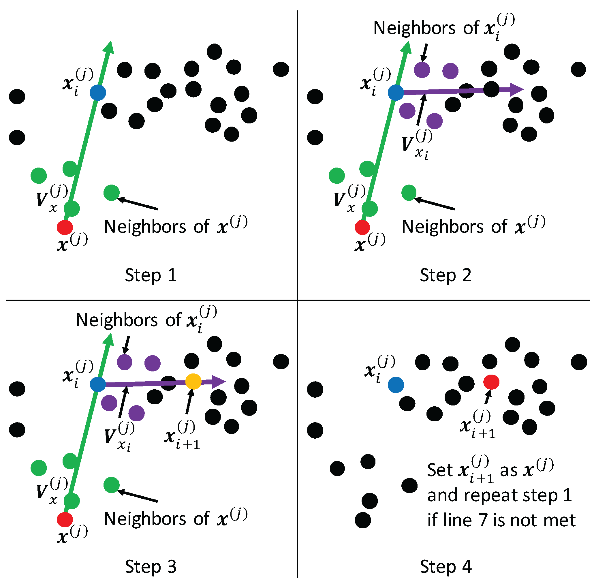
Figure 3.
Synthetic dataset.
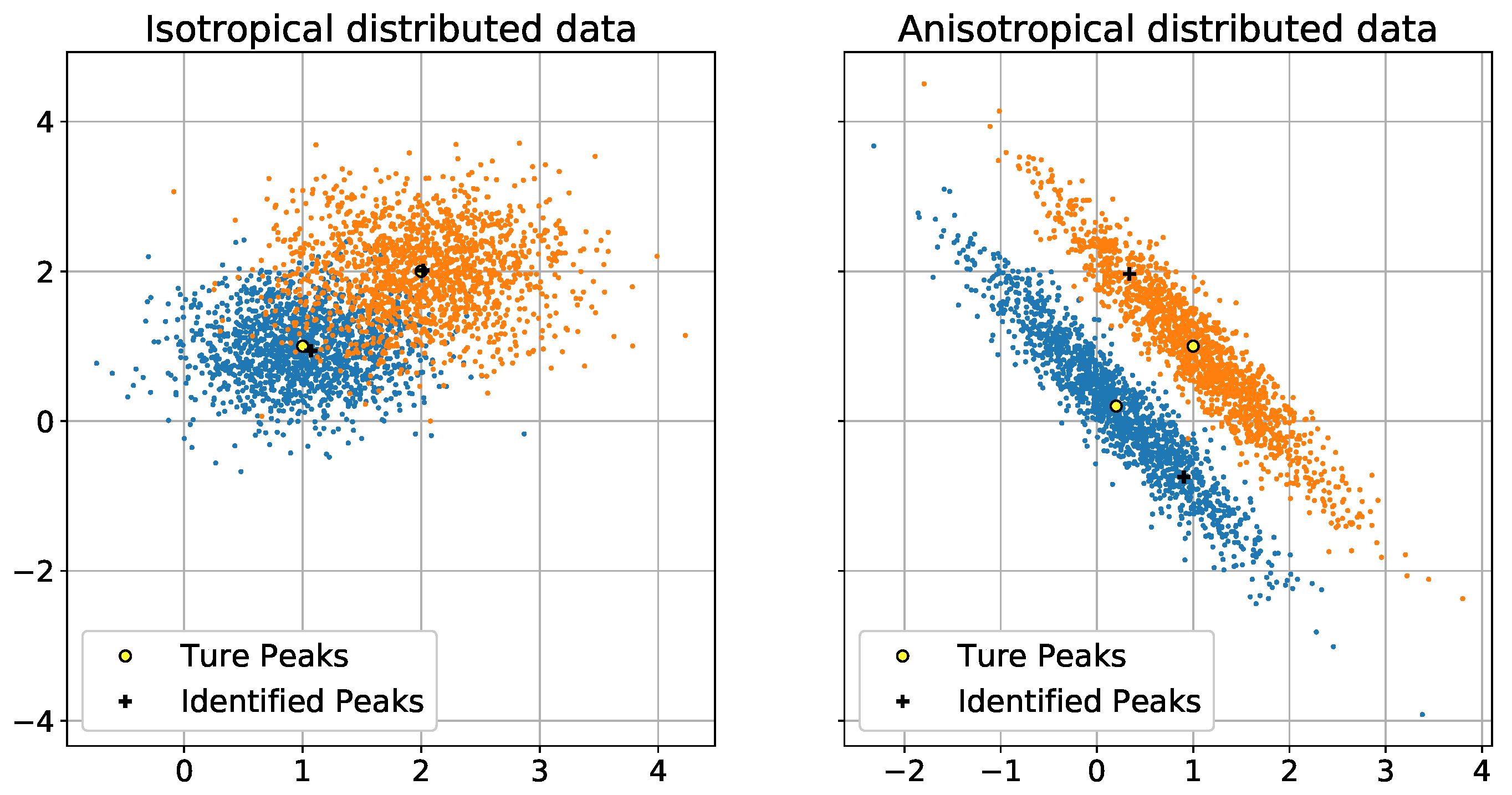
Figure 4.
Comparison of iterations: OEM.
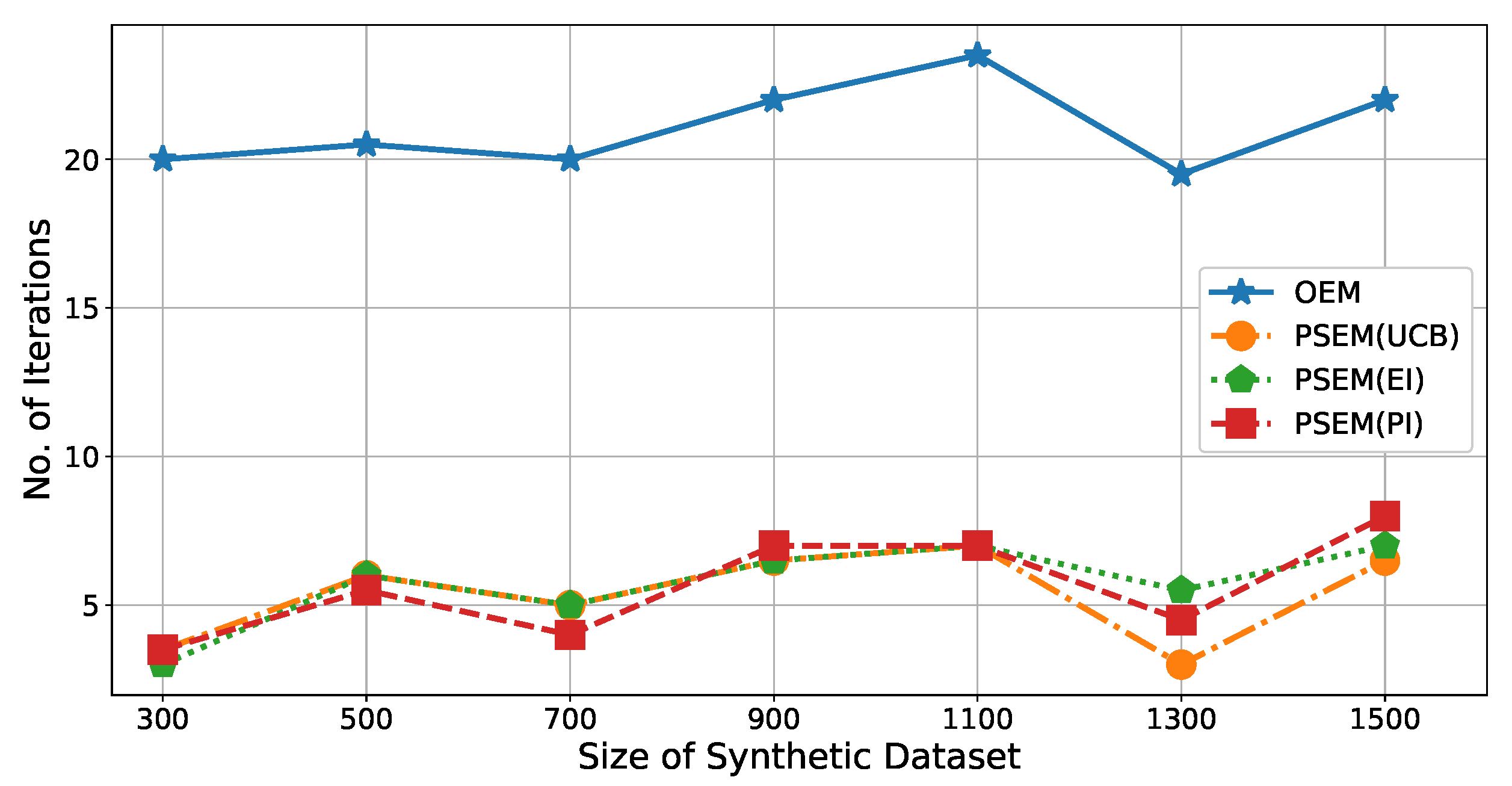
Figure 5.
Comparison of iterations: k-means++.

Figure 6.
Measurements for isotropic dataset.

Figure 7.
Measurements for anisotropic dataset.
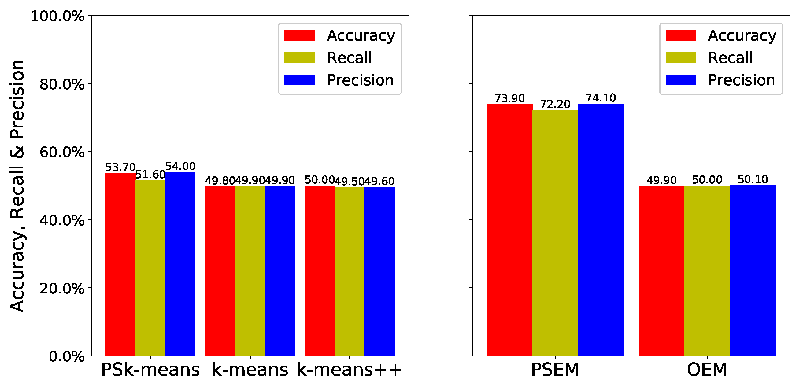
Figure 8.
Dataset from Intel Berkeley Research Laboratory.
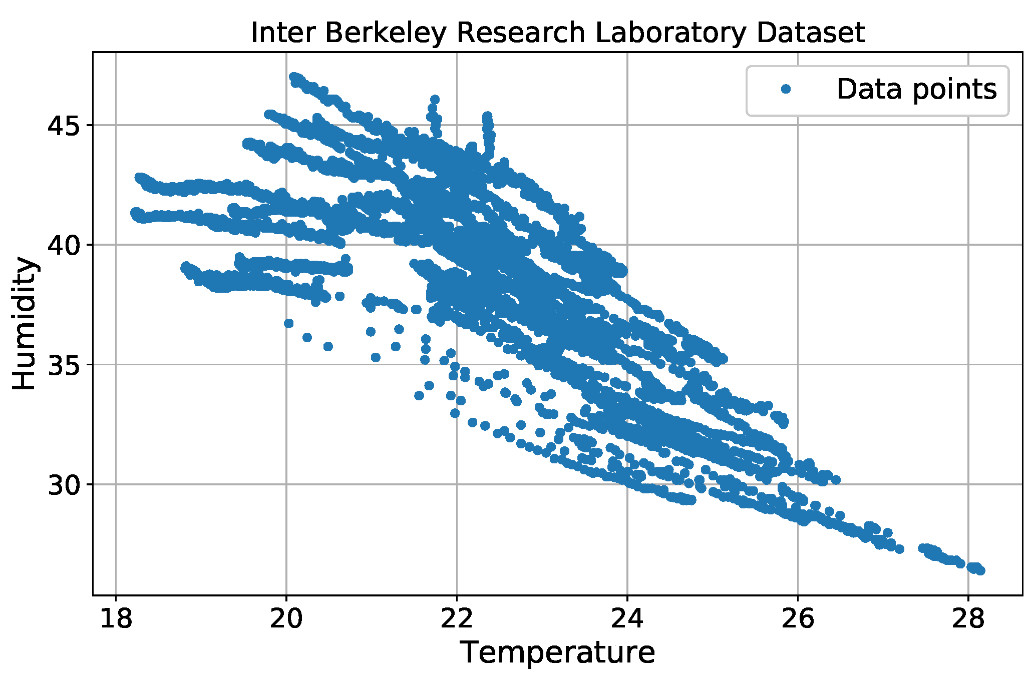
Figure 9.
Floor plan of Intel Berkeley Research Laboratory.
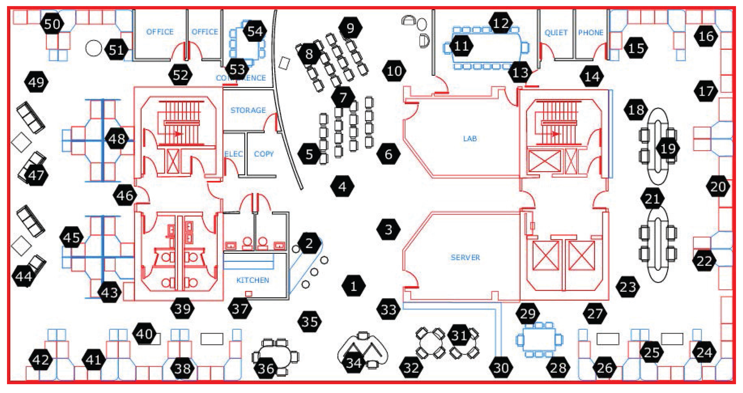
Figure 10.
WSN configuration.
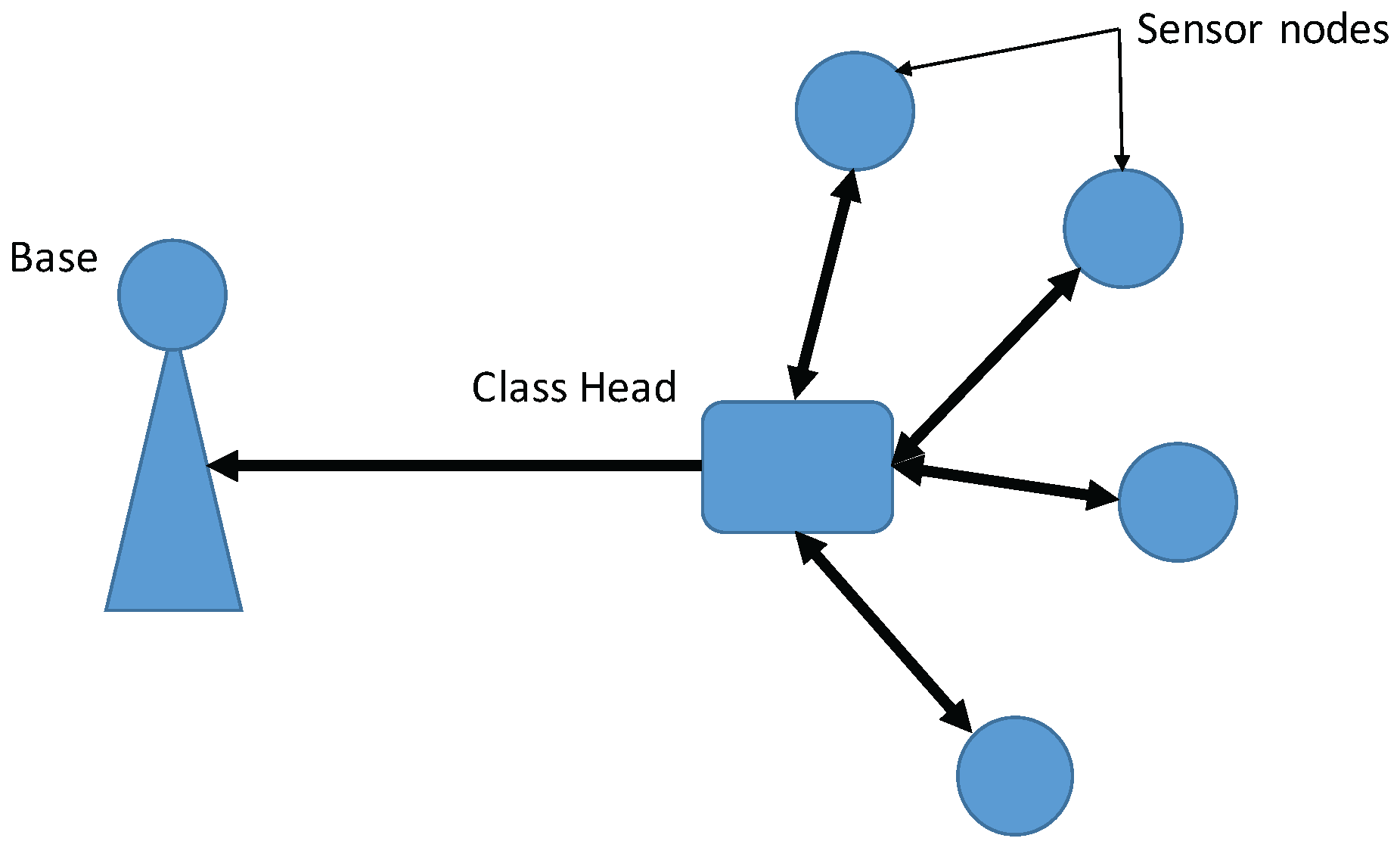
Figure 11.
Accuracy of real dataset.

Figure 12.
No. of iterations for dataset.


Table 1.
Normal data ranges.
| Range | Average | |
|---|---|---|
| Temperature (C) | – | 23.14 |
| Humidity (%) | – | 37.69 |
© 2018 by the authors. Licensee MDPI, Basel, Switzerland. This article is an open access article distributed under the terms and conditions of the Creative Commons Attribution (CC BY) license (http://creativecommons.org/licenses/by/4.0/).
Share and Cite
MDPI and ACS Style
Zhang, T.; Zhao, Q.; Shin, K.; Nakamoto, Y. Bayesian-Optimization-Based Peak Searching Algorithm for Clustering in Wireless Sensor Networks. J. Sens. Actuator Netw. 2018, 7, 2. https://doi.org/10.3390/jsan7010002
AMA Style
Zhang T, Zhao Q, Shin K, Nakamoto Y. Bayesian-Optimization-Based Peak Searching Algorithm for Clustering in Wireless Sensor Networks. Journal of Sensor and Actuator Networks. 2018; 7(1):2. https://doi.org/10.3390/jsan7010002
Chicago/Turabian StyleZhang, Tianyu, Qian Zhao, Kilho Shin, and Yukikazu Nakamoto. 2018. "Bayesian-Optimization-Based Peak Searching Algorithm for Clustering in Wireless Sensor Networks" Journal of Sensor and Actuator Networks 7, no. 1: 2. https://doi.org/10.3390/jsan7010002
Note that from the first issue of 2016, this journal uses article numbers instead of page numbers. See further details here.