
The Realized Hierarchical Archimedean Copula in Risk Modelling

1
Chair of Econometrics and Statistics esp. Transportation, Institute of Economics and Transport, Faculty of Transportation, Dresden University of Technology, Helmholtzstraße 10, 01069 Dresden, Germany
2
Chair of Mathematics and Statistics, University of St Gallen, Bodanstrasse 6, 9000 St Gallen, Switzerland
*
Author to whom correspondence should be addressed.
Econometrics 2017, 5(2), 26; https://doi.org/10.3390/econometrics5020026
Submission received: 31 December 2016
/
Revised: 2 June 2017
/
Accepted: 6 June 2017
/
Published: 15 June 2017
(This article belongs to the Special Issue Recent Developments in Copula Models)
Abstract
:This paper introduces the concept of the realized hierarchical Archimedean copula (rHAC). The proposed approach inherits the ability of the copula to capture the dependencies among financial time series, and combines it with additional information contained in high-frequency data. The considered model does not suffer from the curse of dimensionality, and is able to accurately predict high-dimensional distributions. This flexibility is obtained by using a hierarchical structure in the copula. The time variability of the model is provided by daily forecasts of the realized correlation matrix, which is used to estimate the structure and the parameters of the rHAC. Extensive simulation studies show the validity of the estimator based on this realized correlation matrix, and its performance, in comparison to the benchmark models. The application of the estimator to one-day-ahead Value at Risk (VaR) prediction using high-frequency data exhibits good forecasting properties for a multivariate portfolio.
JEL Classification:
C13; C51; C53; C55; C581. Introduction
One of the main objectives of quantitative research is the modelling and approximation of multivariate distributions. A multivariate model should be flexible enough to capture the stylized facts of empirical finance. Moreover, increasing interest in short-term quantitative risk management requires the time-variability of such models. The current paper builds on two actively developing areas of financial econometrics: copulae and high-frequency data. On the one hand, copulae appear to be a helpful tool to analyse complex dependence structures, evaluate the risk, and are therefore widely used to price financial derivatives, see Embrechts et al. (2003), Rodriguez (2007), Hofert and Scherer (2011), Krämer et al. (2013). On the other hand, models based on high-frequency data yield superior predictions in comparison to approaches based on daily data. Among others, Andersen et al. (2002), Barndorff-Nielsen and Shephard (2004) and Zhang et al. (2005) made it possible to compute the daily realized covariances from high-frequency data. Many researchers have implemented the obtained realized measures to model financial time series. Most of those studies, however, employ models where the realized correlation matrix directly characterizes the multivariate distribution, see, for example, Bauer and Vorkink (2011), Chiriac and Voev (2011), Jin and Maheu (2012), or address GARCH type models, for example, Hansen et al. (2014), Bauwens et al. (2012), Noureldin et al. (2012), Bollerslev et al. (2016). There are only a limited number of studies which discuss the implementation of high-frequency data in copula models. Breymann et al. (2003) and Dias and Embrechts (2004) employ copulae to study the properties of intraday log-returns. Creal et al. (2013) consider an autoregressive updating equation and improve the predictive power in Salvatierra and Patton (2015) by including the lagged realized volatility in the equation.
To the best of our knowledge, the only model that parameterizes the whole Archimedean copula (AC) by the realized variance-covariance matrix is in Fengler and Okhrin (2016), who introduced the realized copula parameter. The authors suggested capturing time-varying dependence by using high-frequency intraday data to estimate the parameter of an AC daily. It has been demonstrated empirically that the realized copula model outperforms the list of benchmark models in one-day-ahead out-of-sample VaR prediction. The realized copula model of Fengler and Okhrin (2016) has, however, several limitations. First, their realized copula is driven by one single parameter, which limits the flexibility of the model. Second, the estimation procedure is performed by applying a method of moments kind of estimator, which suffers from the curse of dimensionality.
We propose to extend the work of Fengler and Okhrin (2016) by introducing the realized hierarchical Archimedean copula (rHAC), which allows more flexibility and is applicable to managing high-dimensional portfolios. We adapt the estimation procedures described in Segers and Uyttendaele (2014) and Górecki et al. (2016a) to high-frequency data, which allows estimating the structure and the parameters of a copula based only on a realized covariance matrix. As a result, the estimate does not suffer from microstructure noise or jumps. Moreover, it can be applied to high-dimensional portfolios since the computationally expensive optimization procedure proposed in Fengler and Okhrin (2016) is reduced to a set of simple tasks. This result is of particular importance in many financial applications, especially in risk management.
This paper is structured as follows. Section 2 contains a literature review of the theory of the copula and introduces the concept of a realized copula. An estimator of the structure and the parameters of an rHAC is presented in Section 3. Simulation studies and a comparison with the benchmark models are provided in Section 4. Section 5 discusses the construction of the rHAC, and gives a short summary of competing models. Section 6 describes an application of the proposed models to one-day-ahead VaR prediction for a multidimensional portfolio. Finally, we summarize the main contribution of the paper.
2. The Concept of the Realized Copula
The concept of the copula was introduced to the statistical literature by Sklar (1959) and further popularized in the world of finance by Embrechts et al. (1999) in the context of risk management. Sklar’s theorem, see Sklar (1959), states that a d-dimensional distribution function with marginals can be represented as
where is a d-dimensional copula. In addition, it states that the continuity of the marginal distributions ensures the uniqueness of the copula.
Having a huge number of classes of bivariate copulae, see Nelsen (2007), there is still a lack of multivariate ones. The most popular classes of multivariate copulae currently are elliptical, factor, pair-copula constructions, and HAC. The first class is often used in practice due to its simplicity and intuitive interpretation. However, elliptical copulae are not able to capture the stylized facts observed in financial data. The factor approach overcomes this limitation and has attracted attention in the copula literature over the last decade, see, for example, Andersen and Sidenius (2004), Van der Voort (2007), Krupskii and Joe (2013), Oh and Patton (2017). The limitation of the factor copula models is that the likelihood function is often not known in closed form, which complicates the estimation of the parameters. Pair-copula constructions are discussed in more detail by Joe (1996), Bedford and Cooke (2001), Czado (2010), and Kurowicka (2011), and are increasing in popularity. Another popular copula class is AC, which contains, among others, the Clayton, Gumbel and Frank copulae. The AC parametrized by the parameter is defined as , with being non-decreasing and convex on for , where . , and the pseudo inverse is defined as for and 0 otherwise. The generators and the densities of some AC are given in Appendix A.
Due to the lack of flexibility of AC, caused by the fact that the whole copula is driven by just one parameter , generalizations such as nested copulae have been introduced. This paper employs a flexible multivariate copula family, HAC, a special case of which may be defined recursively in the following way:
where is the parameter vector of the HAC and s is the structure of the HAC. As is evident from (2), the current study assumes that all generators of the HAC belong to the same parametric family and each of them depends on one single parameter. For simplicity, we compress the notation of (2) and denote the d-dimensional HAC with k generators which is parametrized by the structure s and the parameter vector as . The structure s is the merging ordering , where , is a reordering of the indices of the variables , . The structure of a d-dimensional HAC s can be seen as a tree with non-leaf nodes that correspond to the generators and d leaves representing the variables . The leaves correspond to the lowest level of the tree. The root corresponding to the variable is assumed to be the highest level of the tree. The nodes, which are not the leaves are called internal nodes, each corresponds to the generator. A node which is directly connected to another node when moving away from the root is called the child node. A node which is directly connected to another node when moving from the leaves to the root is called the parent node. Descendants are the children nodes of the node, children of these children, etc. The set of ancestors includes the parent node of the node, parents of the parents, etc. The structure of the HAC is called binary if it corresponds to the binary tree, i.e., if each internal node has exactly two children. Further on, we denote the nodes associated with the generators by , where is the set of leaves (variables) that are descendant nodes of the node , . Assuming this notation, the node is an ancestor of the node (the leave associated with the variable ) if (), , . Another concept that will be used later on is the concept of the lowest common ancestor (lca). The lca of the nodes (the leave ) and (the leave ) is the node that is the lowest node satisfying () and (), , .
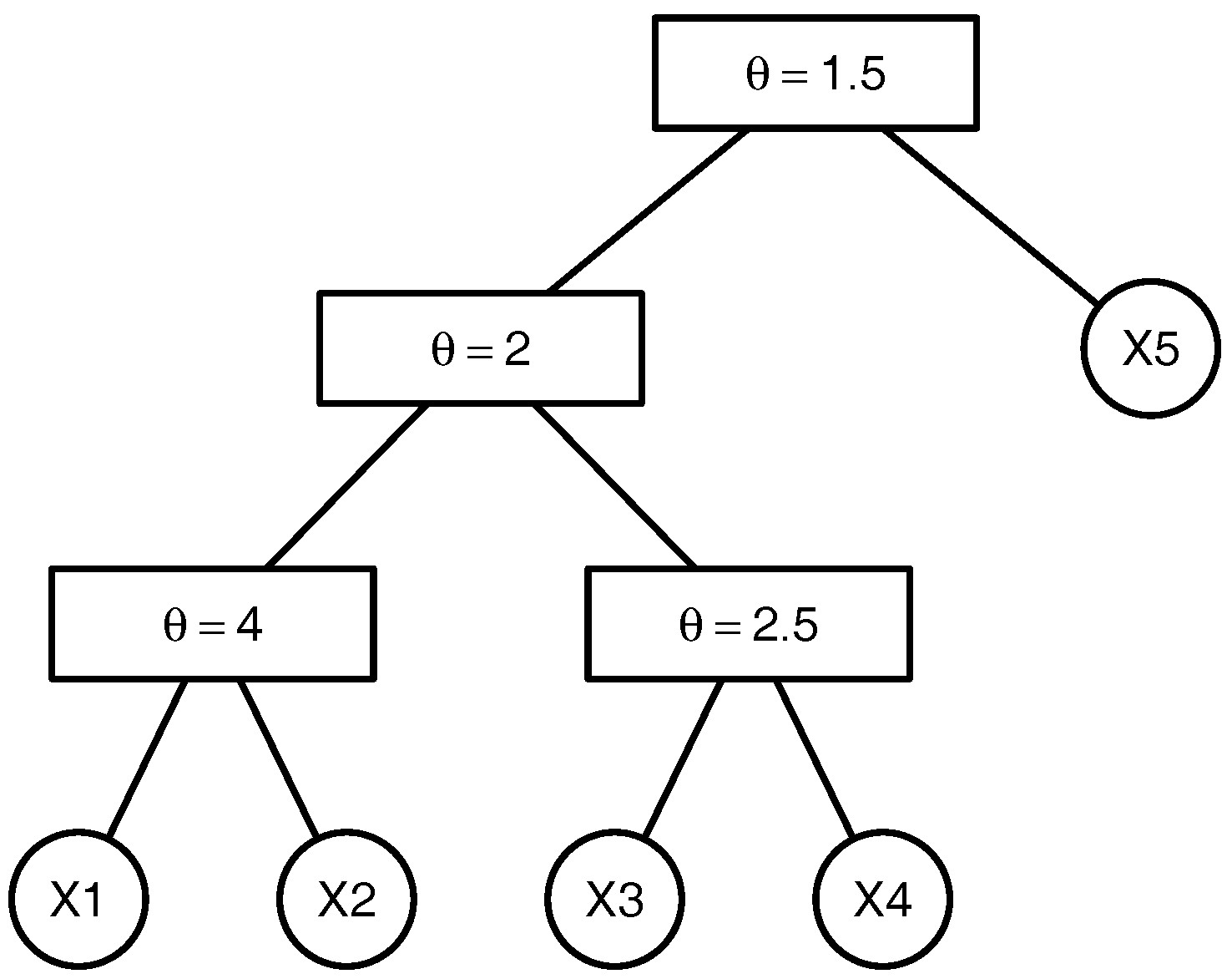
To clarify the above-mentioned definitions and avoid introducing the comprehensive notation of the graph theory, we illustrate the above-named concepts by an example. Consider the 5-dimensional copula
that can be written as , where with being the parameters of the marginal distributions , . The tree corresponding to this copula is presented in the Figure 1. This copula has the binary structure . There are non-leaf (internal) nodes. The leaves which correspond to the lowest level of the copula tree are given by the variables , , , and . The root which represents the highest level of the copula tree corresponds to the variable , where . The root node is the parent node for the node corresponding to the variable and the node associated with the variable generated by , where . The root node is the ancestor for all other nodes of the given copula tree. The lca of the nodes associated with the variables and is the node that corresponds to the variable , where . The lca of the nodes corresponding to the variables and is the root node as it is the lowest node satisfying and , .
Although copula models are flexible enough to capture nonlinear dependencies, many empirical applications require the time variability of the parameters (and the structure) of the whole copula. For example, the empirical evidence makes it reasonable to assume that the dependence between asset log-returns gets stronger during periods of financial turbulence. A vast amount of literature is devoted to dynamic copula models, including the parsimonious rolling window approach and more sophisticated models, such as, for example, the local change point procedure of Härdle et al. (2013). Recent developments in time-varying copula models take advantage of the rapidly growing availability of high-frequency observations and include the realized measures (volatility and correlations) in the copula models to improve their predictive power, see, for example, Salvatierra and Patton (2015). The improvement is obtained due to the fact that the actual realizations of the volatility of log-returns which are not directly observable can be estimated by the sum of finely-sampled squared realizations of log-return over a fixed time interval when the high-frequency observations are available. Such a nonparametric ex-post measurement of the log-return variation is called the realized volatility. In an analog manner, the realized covariances are defined by summing all the cross products of intraday log-returns. The formal definition of the realized measures is given in Appendix B. Despite the constantly growing research on incorporating the realized measures into multivariate Gaussian models, discussed in Chiriac and Voev (2011) and Bauer and Vorkink (2011), and into GARCH type models, for example, Hansen et al. (2014) and Bollerslev et al. (2016), there is still a gap in the literature on how the parameters of non-Gaussian copula can be estimated daily based on high-frequency observations. It is important to note here that such standard copula estimation techniques as the Maximum Likelihood (ML) method or the inversion of Kendall’s can not be directly applied to tick-by-tick observations. Estimating the copula by applying these approaches to high-frequency data would estimate the multivariate distribution of high-frequency log-returns, which in general does not coincide with the multivariate distribution of daily log-returns. Such a model would estimate the intraday dependence and produce the forecast of the multivariate distribution of log-returns in the next second and could not be used for one-day-ahead VaR forecasts. For further details on the standard estimation procedures, refer to Nelsen (2007), Trivedi and Zimmer (2007), Jaworski et al. (2013), Cherubini et al. (2011), Joe (2014) and Durante and Sempi (2015). In contrast to the direct application of the ML approach to tick-by-tick data or high-frequency estimator of Kendall’s , there is a considerable literature discussing how to estimate the correlation matrix of daily log-returns via a realized correlation matrix or similar methods, see Barndorff-Nielsen et al. (2004), Barndorff-Nielsen and Shephard (2004), Zhang et al. (2005), Hayashi and Yoshida (2005), De Pooter et al. (2008). The idea of using the information concentrated in the realized covariance matrix to estimate the parameters of a copula daily has been employed by Fengler and Okhrin (2016), who used a combination of the results from a lemma of Hoeffding (1940) and Sklar’s theorem (1) to express the covariance between two random variables and in terms of the marginal distributions and and the copula
where is the parameter of the copula and , are the parameters of the marginal distributions and . In the high-frequency framework, the covariance in (3) is replaced by the element of the realized covariance matrix computed at day t. From now on, we denote the diagonal elements of matrix by instead of , . As has been shown in Breymann et al. (2003) and discussed in more detail in Hautsch (2011), with an increasing sampling frequency, the marginal distributions of log-returns can be assumed to be Gaussian with zero mean and the standard deviation equal to , , this leads us to assume throughout this study that margins are . Thus, if the realized covariance matrix can be computed, according to Fengler and Okhrin (2016), it can be assumed that for the Archimedean copula driven by one single parameter the integral in (3) depends on just the parameter of the copula which belongs to some parametric family . Therefore, after replacing the covariances in (3) by their realized counterparts and standardizing the variables, the expression (3) can be rewritten for the realized correlations as
where is the cdf of the standard normal distribution and is the element of the realized correlation matrix calculated at day t, . According to (4), the realized correlations depend solely on the copula parameter, under the assumption of some parametric family. Based on (4), the parameter of the copula can be estimated based on just the realized correlation matrix:
where is a vector of length where all the are stacked together and W is a -dimensional positive definite weighting matrix. When the copula parameter is estimated from (5) and the diagonal elements of the realized covariance matrix are calculated, the multivariate distribution of is fully specified. It is important to note that Fengler and Okhrin (2016) consider the restrictive setting of AC. Therefore, all bivariate copulae in (4) coincide and are driven by one single parameter .
In practice, one is usually interested in predicting a multivariate distribution, rather than just estimating it. This can be done in two ways. The parameter of the realized copula can be estimated daily and predicted using some time-series model. Alternatively, the realized correlation matrix can be predicted and the parameter of the copula can be estimated from , which is one-day-ahead prediction of the realized correlation matrix obtained by applying the specific time series model in the spirit of Bauer and Vorkink (2011) or Chiriac and Voev (2011). The limitation of both approaches comes from the estimation procedure (5), which suffers from the curse of dimensionality and enables the estimation of the realized copula only in moderate dimensions. Moreover, as was mentioned earlier, the whole realized copula in Fengler and Okhrin (2016) is driven by just one parameter , which might be too restrictive for multivariate portfolios.
We propose to overcome these limitations by using the HAC instead of the simple AC. This extension is not straightforward, as in addition to the parameter vector of , the structure of the copula s needs to be estimated. The estimation of the parameter vector of a d-dimensional copula should be addressed as well. The procedure of Fengler and Okhrin (2016) allows the estimation of the parameters at the bottom level of the copula. The estimation of the parameters of the higher levels is not trivial, as the realized correlation among the original variables and the variables determined by the copulae of the bottom levels can not be specified. This motivates the estimation of the structure and the parameters of the hierarchical copula based just on the realized correlation matrix. Recent studies in the copula literature address the question of how the structure (or the structure and the parameters) of a hierarchical copula can be estimated based on Kendall’s correlation matrix, see, for example, Segers and Uyttendaele (2014), Górecki et al. (2016a, 2016b), Uyttendaele (2016). We propose to combine the methods discussed in Segers and Uyttendaele (2014) and Górecki et al. (2016a) and adapt them to the realized correlation matrix with the final goal of improving one-day-ahead VaR prediction for multivariate portfolios.
3. Estimating the Realized Hierarchical Archimedean Copula
This section discusses how the structure and the parameters of an HAC can be estimated based on the realized correlation matrix only. From now on, we refer to such a copula as an rHAC. In this section, the subindex t is dropped to simplify the notation. We suggest generalizing the clustering method proposed by Górecki et al. (2016a) by applying an adaptation of the algorithm introduced in Segers and Uyttendaele (2014) in order to estimate the structure of an HAC. Consequently, the parameters can be estimated by applying (4) to the specific average of the realized correlations. We restrict ourselves to the case when all the generators of the copula belong to the same Archimedean family and satisfy the nesting condition. A brief discussion of this will be provided later in this section.
3.1. Estimating the Structure
In analog to the method mentioned in Górecki et al. (2016a) for Kendall’s , we suggest defining the distance between two variables and as
where is the realized correlation between and , . Next, the dependence-based distance matrix is used as the input for an agglomerative cluster analysis. The obtained hierarchical clustering dendrogram corresponds to the estimated structure of the HAC. This approach is, however, valid only for HACs with binary (bivariate) structure. The introduction of an additional merging parameter that allows collapsing a binary structure into a general one is discussed in Uyttendaele (2016). The optimal choice of such a parameter still needs to be addressed in the literature. To reduce the computational costs, we will adapt the method proposed in Segers and Uyttendaele (2014) to the distance (6) to recover the general structure of an rHAC.
3.1.1. Segers’ and Uyttendaele’s Algorithm
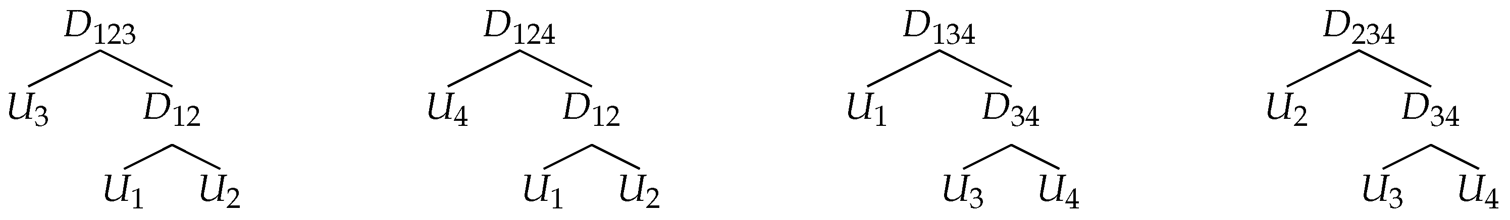
According to Segers and Uyttendaele (2014), the structure of a nested HAC s can be uniquely recovered from the structures of the set of triples with distinct using the concept of lca. According to the definition given in Section 2, the lca of and is the node which is the lowest node that has both and as descendants, . In the first step, the structures of the triples are estimated and the lcas of all pairs of variables in each triple are found. For a given tree, there are lcas that correspond to all possible pairs , . In the second step, the pairs of variables which correspond to the same equivalence class are merged together step by step, resulting in the tree of the HAC. Two pairs of variables and are said to belong to the same equivalence class if they share the same lca in the tree s.
As an example, we consider the 4-dimensional HAC with the predefined structures of the triples presented in Figure 2. Consider the first triple with the structure . The lca of is the node . For simplicity of notation, we write instead of . The parent node of and is given by . The ancestor nodes of and are the nodes and . Therefore, the lca of in the structure is the node and the lca of is the node . The lcas of each pair are:
In the given example, the pairs and do not share lcas with any other pair. Therefore, and belong to the same equivalence class and are merged together in the first step. The same is true for the pair . Consequently, it is observed that the pairs , , and belong to the same equivalence class and are merged together in the second step. The final structure of the copula is . For further examples on how the structure of an HAC can be recovered by applying the concept of an lca, we refer to Segers and Uyttendaele (2014).
In this method, the structure of the individual triples should be found first. Each triple can have a binary or a trivial structure. The structure of the triple is called trivial if all three variables are merged together in one step, and binary otherwise. Formally speaking, for each triple of variables , we aim to test the null hypotheses ‘the structure is trivial ’ against ‘the structure is binary ’. Segers and Uyttendaele (2014) suggest estimating the individual triples using a rank-based method. Let be Kendall’s distribution between and . Its empirical counterpart is then where , and is the identity function. The distance between the empirical Kendall distributions of pairs and is defined as
where are ordered pseudo-observations of . Segers and Uyttendaele (2014) point out that a trivial trivariate structure usually results in three distances which are approximately the same, but a binary structure results in one small distance and two larger approximately equal distances. In order to calculate the test statistic, Segers and Uyttendaele (2014) suggest drawing K samples from the nonparametrically estimated trivariate Archimedean copula using the work of Genest et al. (2011).
As the present paper addresses the framework when the copula family is assumed to be known, we modify the algorithm proposed in Segers and Uyttendaele (2014) and simulate from the copula coming from a predefined class. The test statistic is simulated under the assumption that the structure is trivial, therefore, the parameter of the copula can be found by inversion of the average empirical counterpart of Kendall’s , i.e., , where , . The inverse corresponds to the solution of the equation
where with and are independent draws from . For some copula functions, the integral in (8) is known in closed form as a function of , for example, for the Gumbel and Clayton copulae and , respectively. To sum up, the modification of the algorithm of Segers and Uyttendaele (2014) which allows identifying the structure of an HAC based on Kendall’s distance is summarized in Algorithm 1.
| Algorithm 1 Adaptation of the algorithm of Segers and Uyttendaele (2014). |
| Input: sample of size n, significance level , parametric family of the HAC. |
| for do |
| ⊳ Select a triple from , , , call it . |
| ⊳ Compute the distances , and according to (7), order them and call the result . |
| ⊳ Compute the test statistic
|
| ⊳ Compute and estimate according to (8). |
| for do |
| ⊳ Draw a sample of size n from being a trivial copula. |
| ⊳ Compute for the simulated sample k in analog to (9). |
| end for |
| ⊳ Compute by taking the quantile of the empirical distribution of , . |
| if then reject the : the true trivariate structure is the trivial structure. |
| end if |
| end for |
| ⊳ Recover the full structure of the d-dimensional HAC from the set of triples of variables using the concept of the lowest common ancestor (lca). |
| Return: the estimated structure of the HAC . |
The significance level of the individual tests should be selected considering the multiple testing procedure. For the significance level of the test to be , the significance level of the individual tests should satisfy . However, this approach is not recommended for high-dimensional samples. Therefore, in the empirical part of the paper, we use the rule of thumb proposed in Uyttendaele (2016) and choose the significance level of the individual tests to be smaller or equal than the overall significance level. It is worth noting that the method of Segers and Uyttendaele (2014) is much more general as no prior specification of the copula generators is necessary and generators might differ from level to level of the hierarchy. In contrary, our method assumes that generators on all levels of the hierarchy belong to the same predefined family. However, the method proposed in Segers and Uyttendaele (2014) and its modification described in Algorithm 1 are not applicable to the case of high-frequency data because of the absence of a high-frequency estimator of Kendall’s and Kendall’s distribution. The computation of the empirical Kendall’s distribution (7) involves realizations of . Therefore, the estimation of a multivariate distribution of daily observations would require data of a longer time horizon in comparison to the case when the copula is parameterized by solely the realized correlation matrix. The structure and the parameters would have to be fixed within some time window, resulting in the reduced time flexibility of the estimated multivariate distribution. Moreover, Algorithm 1 employs Kendall’s distance as the test statistic, which leads to large computational costs in higher dimensions.
3.1.2. Clustering Estimator of the Structure
We propose to proceed analogously to Segers and Uyttendaele (2014) and recover the full structure of an HAC from the set of triples of variables. The estimation of the structure of the individual triples is made using a test that, in contrast to Segers and Uyttendaele (2014), does not involve the observations themselves and is based solely on pairwise correlations.
Consider the triple and assume that the estimated distance , where is defined in (6). Therefore, the variables and are merged together into the variable in the first step. The distance between the cluster and is calculated according to the complete linkage rule:
Preliminary simulation studies have shown that the choice of the clustering algorithm is of minor importance. We refer to Kaufman and Rousseeuw (2005) and Hastie et al. (2009) for more details on cluster analysis.
It can be observed that the difference between merging distances and is generally bigger if the trivariate copula has a binary structure. Therefore, the measure
can be chosen as the test statistic to distinguish between trivial and binary structure of a triple.
To sum up, the testing procedure is performed in the following way: for each triple, it is assumed that the structure is trivial, the average correlation is computed, and inverted to the parameter of the trivial copula according to (4). The test statistic is obtained by simulating samples from the trivial copula and calculating K distances according to (11). The sample size of the simulated sample corresponds to the sample size of the original sample. Finally, the empirical difference of the merging distances is compared to the quantile of the simulated one. The proposed procedure is briefly summarized in Algorithm 2.
| Algorithm 2 Structure determination using cluster analysis. |
| Input: the realized correlation matrix of the dimension calculated based on the sample of size n, significance level , parametric family of the HAC. |
| for do |
| ⊳ Select a triple from , , , call it . |
| ⊳ Compute , , and according to (6). |
| ⊳ Merge the two closest variables and calculate according to (11). |
| ⊳ Compute and estimate . |
| for do |
| ⊳ Draw a sample of size n from being a trivial copula. |
| ⊳ Transform to . |
| ⊳ Compute for the simulated sample k according to (11). |
| end for |
| ⊳ Compute by taking the quantile of the empirical distribution of , . |
| if then reject the : the true trivariate structure is the trivial structure. |
| end if |
| end for |
| ⊳ Recover the full structure of the d-dimensional rHAC from the set of triples of variables using the concept of the lowest common ancestor (lca). |
| Return: the estimated structure of the HAC . |
It is important to note that the estimation of the marginal distributions is a trivial task, as the distribution of the high-frequency log-returns can be assumed to be Gaussian , based on the results described in Hautsch (2011).
Note:
In order to illustrate the test statistic (11), samples from and are drawn (the copulae are assumed to be Gumbel). The left plot in Figure 3 illustrates the dendrogram of the hierarchical cluster analysis based on the distance (6) and complete linkage merging rule for a random sample of size 100 from the trivial Gumbel copula. The central part of Figure 3 shows the dendrogram for the binary trivariate Gumbel copula. It can be observed that the difference between merging distances is much smaller for the trivial copula. We simulated random samples from each of the above mentioned copulae, and each time calculated according to (11). The kernel density estimate of the based on 100 random samples is presented in the right part of Figure 3. For the given copulae, the density estimate of for the trivial copula is more concentrated. This example only illustrates the validity of the proposed test statistic. The distance between these two distributions is influenced by the values of the parameters, and more research should be done to find the asymptotic properties of the proposed test.
3.1.3. Benchmark Models
Many recent studies have addressed the question of the structure’s estimation of an HAC, for example, Okhrin et al. (2013, 2015), Górecki et al. (2014, 2016b) and Uyttendaele (2016). Most of the studies illustrate the performance of the proposed methods by means of simulations. The consistensy of the structure’s estimator still has to be addressed in the literature. Some of these studies are much more general than Algorithm 2. However, they are not applicable in the current framework, where the observations can not be directly used, as discussed in the previous section. Moreover, in the overwhelming majority of cases, the methods perform in a similar way for big samples. To illustrate the validity of Algorithm 2, it will be compared, by means of simulations, to the recursive procedure proposed in Okhrin et al. (2013) and further improved by Górecki et al. (2014). It has been implemented in the R package HAC by Okhrin and Ristig (2014). The idea of the method is to construct a binary tree by recursively merging the variables with the largest values of the estimated parameter. Subsequently, the obtained tree is collapsed using a predefined merging parameter. As is the case with many others, this method can not be applied to high-frequency data. However, it will provide an opportunity to evaluate the loss of precision and gain in computational speed when the general structure is estimated based solely on the realized correlation matrix.
3.2. Estimating the Parameters
As was mentioned in Section 2, the parameters of the copula can be estimated by the inversion of the realized correlation according to (4). However, this is usually done only for the correlation between two variables. Some generalizations for Kendall’s have already been addressed in the literature. Nelsen (1996) discusses how the parameter of a three-dimensional binary copula can be found by inverting the average coefficient of agreement. Genest et al. (2011) have described the average Kendall’s based approach to the trivial copulae with an odd number of parameters. Górecki et al. (2016a) mention the estimation of the parameters of a binary HAC based on Kendall’s correlation matrix and discuss a trivial extension to HAC with general structures in Górecki et al. (2016b).
We suggest following the idea of averaging the correlation coefficient , over some given set of variables to estimate the parameters of the rHAC. The question whether the procedure based on the average realized correlation gives a valid estimate has not been addressed in the literature.
Suppose that k parameters of the HAC , corresponding to k merging nodes need to be estimated. Let be the average correlation of the pairs of variables with the lca at node , , where is the set of descendant leaves (variables) of the node , . Thus, the parameter of the HAC may be estimated by inverting the average correlation measure , . For the HAC with the structure presented in Figure 1, the node associated with the parameter is the node . The children nodes of the node are the nodes and . The node is associated with the parameter and the node is associated with the parameter . Moreover, the node is the ancestor for the nodes associated with the variables , , and . The lca of the pair is the node and the lca of the pair is the node . Therefore, the pairs of variables with the lca at node are , , and . Therefore, the average correlation corresponding to the parameter is given by . The parameter is estimated by inverting the mentioned above average correlation, i.e., . Analogically, , . A summary of the estimation procedure is given in Algorithm 3.
| Algorithm 3 Average correlation estimator |
| Input: the realized correlation matrix , the estimated structure from Algorithm 2, parametric family of the HAC. |
| ⊳ Let be the set of the HAC parameters to be estimated. |
| ⊳ Let , be the set of the descendants of the node ; is the set of all variables. |
| for do |
| end for |
| Truncate the parameters according to the nesting condition, i.e., , if , . |
| Return: estimated parameter vector of the HAC. |
Simulation studies show that the proposed estimator is asymptotically unbiased and follows a Gaussian distribution. In the case when the realized correlation is replaced by Kendall’s correlation and the parameter is estimated by applying (8) to the average Kendall’s . Let be the average empirical Kendall’s of the pairs of variables with the lca at node and is defined analogically to (12). Let be a set of the pairs of variables with the lca at node , i.e., , , , then the asymptotic variance of the average Kendall’s associated with the node and the parameter can be estimated as
and , where is the survival copula and is the cardinality of the set L. Combined with the expression (8), this implies
The estimator of the variance is a straightforward application of the result developed in Genest et al. (2011).
4. Simulation Results
In this section, we show the validity of the clustering estimator (CE) presented in Algorithms 2 and 3 and compare it to the adaptation of the method of Segers and Uyttendaele (2014) (SU) and the approach of Okhrin et al. (2013) (OOS) which was improved by Górecki et al. (2014) and was implemented in the R package HAC by Okhrin and Ristig (2014). We compare the introduced estimator only to a couple of currently available studies and leave the recent advances discussed in, for example, Górecki et al. (2014, 2016b), Uyttendaele (2016) and Okhrin et al. (2015) outside the scope of this study since the objective of the simulation studies is rather to answer the question whether the proposed algorithm is valid in the case of linear correlation, than to find the best possible estimator of an HAC. We are aware of the fact that the linear correlation based estimator might be not as efficient as an ML approach or a nonlinear correlation based estimator, as it contains information only about linear dependencies among the variables. However, in the framework of high-frequency data, this is so far the only possible way to proceed. Moreover, we aim to define a minimal recommended sample size.
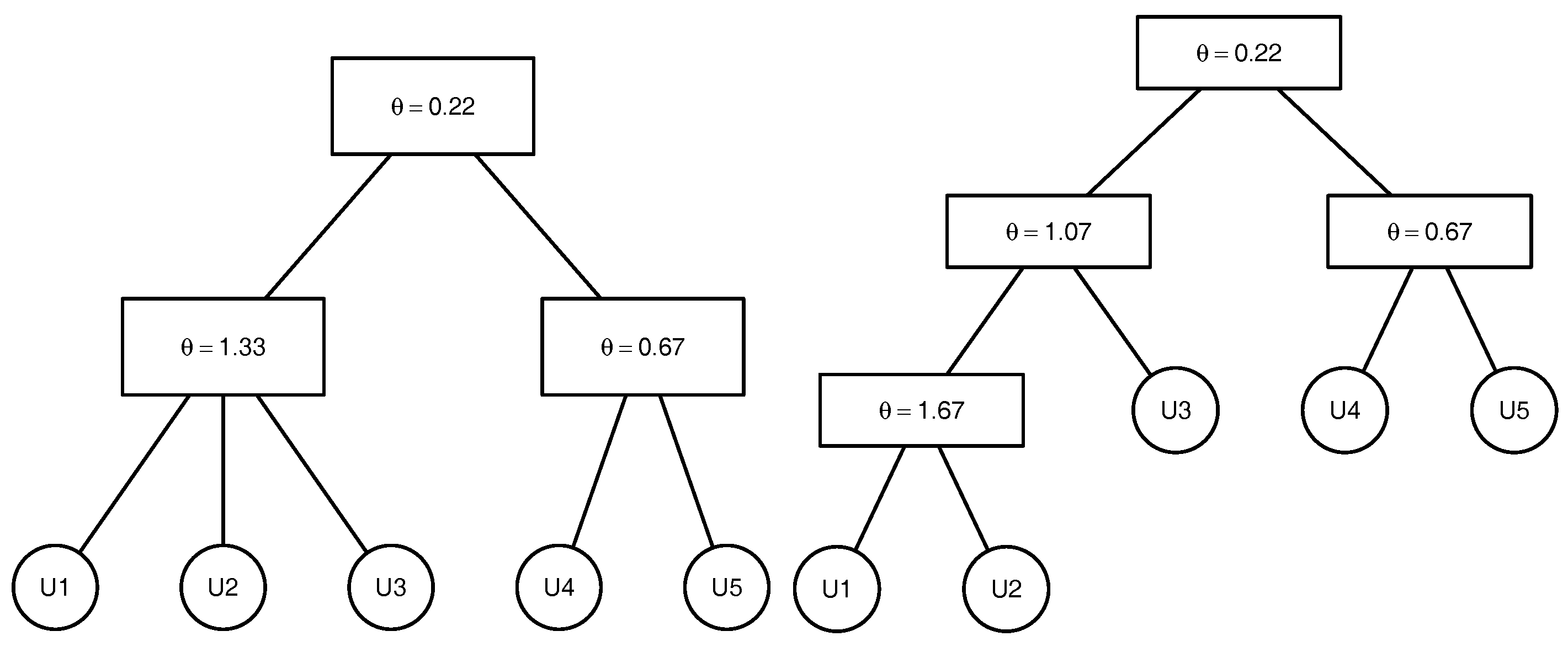
In the current simulation study no high-frequency observations are presented. In order to compare different methods, CE is applied to the Kendall’s correlation matrix and to the linear correlation matrix estimated in the usual manner over the whole sample path that corresponds to the correlation matrices of the daily log-returns. In the case of the SU estimator, the parameters are estimated by the sequential inversion of Kendall’s . For the estimation of the structure according to Algorithms 1 and 2, we set and . A full ML is applied to the structures estimated by OOS. For illustrative purposes, the 5-dimensional copulae structures presented in Figure 4 are considered. For each structure, Clayton, Gumbel and Frank copulae are analysed with the parameters corresponding to and . The marginal distributions are assumed to be known. For each of the above mentioned estimators, we proceed as follows: a sample of size n is simulated from the copula, and the structure is estimated. If the estimated structure coincides with the true one, the parameters are estimated. The procedure is repeated m times until 200 structures are estimated correctly. Thus, the estimators of the structure are compared in terms of the proportion of correctly estimated structures 200/m. For the comparison of the estimation of the parameters, we introduce the characteristic , which is the Euclidean norm of the difference between the vector of true parameters and the estimated ones. Table 1 and Table 2 present the mean , the variance and the 25% , 50% and 75% quantiles of E for different structures.
Table 1 shows the simulation results for the 5-dimensional Clayton copula presented in Figure 4 with sample sizes . The results make evident that the OOS method outperforms all the competitors for small samples for the Clayton copula with the structure . However, there are some outliers, which can be seen from the sample variance of E. This means that the full ML estimate had a large deviation from the true value of the parameter for a few samples. The interquantile range is still smaller for the ML in small samples. The same results for the variance are observed for the CE , therefore, this estimator is not recommended for small samples. In contrast, Table 2 shows that for the structure , OOS is not the best method for estimating the structure in small samples. This is due to the fact that the performance of this estimator depends on the choice of the merging parameter. The results for the other copulae are presented in Appendix C and show that there is no leading method in terms of estimating the structure. The method to choose depends on the type of the copula and the values of the parameters. For a large enough sample, all the methods perform similarly. The general conclusion to be drawn for the estimation of the parameters is that the variance of the CE r estimator is the highest for small samples and that the full ML has the smallest variance, however, some exceptions are observed. It is worth noting that the simulation results are used just for comparison purposes, as the difference in the parameters influences the proportion of the correctly estimated structures more severely than does the type of the copula. Additionally, the dimension of the copula should always be taken into consideration in order to select the minimal sufficient sample size. The question of convergence of the estimator to the true structure still needs to be addressed in the literature.
In Figure 5, we take a closer look at the individual components of . We compare only CE based on Kendall’s correlation and the full ML, as the CE and SU behave very similarly in terms of the properties of . It is evident that both estimators are asymptotically unbiased, however, CE has a higher variance. In addition to the kernel density estimates of CE and ML, we add a kernel density estimate of the Gaussian sample (blue line) with the mean and the variance estimated from (14) and observe that it coincides with the kernel density estimate of CE.
It is worth noting that the computational advantage is on the side of CE. Figure 6 shows the average computational time in seconds for all the above mentioned estimators over 100 trials. The difference in the computational time becomes crucial with growing dimensions, for example, in Segers and Uyttendaele (2014), the SU estimation of a 7-dimensional copula needs roughly 20 min versus 15 s for the proposed clustering estimator (CE).
The main conclusion of this section is that the linear correlation based clustering estimator is applicable in practice and can be applied to high-frequency data, where moderate samples are atypical.
5. Forecasting VaR Using High-Frequency Data
5.1. Predicting rHAC
The model introduced in this section extends the work of Fengler and Okhrin (2016) to higher dimensions. The computationally expensive estimating procedure (5) is reduced to a set of simple tasks of the form (13). Moreover, this procedure allows avoiding the question of the optimal choice of the weighting matrix W in (5).
As mentioned in Section 2, the combination of a lemma of Hoeffding (1940) and Sklar’s theorem (1) allows to express the pairwise covariances in terms of the copula and the corresponding marginal distributions. Under the assumption that the marginal distributions , , are Gaussian , the multivariate distribution of daily log-returns is parametrized solely by a -measurable covariance matrix . This is due to the fact that the structure and the parameters of the HAC are estimated from realized correlation matrix using Algorithms 2 and 3 and the margins are fully specified by the realized volatilities , , i.e.,
where . The prediction of the multivariate distribution of daily log-returns is based on the predicted realized covariance matrix obtained by the Heterogeneous Autoregressive (HAR) model introduced by Corsi (2009) and applied in the spirit of Bauer and Vorkink (2011). First, the individual elements of the realized covariance matrix are stacked together into a joint matrix. Then, the matrix logarithm is calculated to guarantee that the matrix is positive definite. In the next step, the covariances are stacked into one vector and modeled using the logarithmic version of the HAR model:
where , , , and is an error term. When the coefficients in (16) are estimated using ordinary least squares, the prediction is obtained. The prediction is obtained by applying the reverse vech-operator to and taking the matrix exponential . The prediction of the realized correlation matrix is obtained by dividing the elements of by the product of the square roots of the corresponding predicted realized volatilities, i.e., . Since we consider only one-day-ahead prediction, we assume that the prediction bias caused by the nonlinear transformation is small and omit the bias adjustment, analogously to Chiriac and Voev (2011).
We stress once again that only the realized correlation matrix is used for the estimation procedure. The computational costs of such an estimator are low, and the rHAC model still shows excellent forecasting properties.
5.2. Competitor Models
In order to show a competitive advantage of the rHAC, we apply it to one-day-ahead VaR prediction for a multidimensional portfolio and compare the performance of the rHAC to three classes of benchmark models:
- Rolling window copula models
- Dynamic copula models
- -
- -
- -
- Realized covariance model by Bauer and Vorkink (2011)
The first class employs copula models with parameters fixed over the given time interval. The second includes dynamic copula models which assume that the parameter of the copula follows some autoregressive process. The third class, which is both popular and successful, comprises the realized volatility models. A more detailed description of the benchmark models is given in Appendix E.
6. Application
This section illustrates the rHAC model using high-frequency log-returns of stocks traded on the New York Stock Exchange. First, we give a description of the data used in the empirical part of this section. Thereafter, we apply the rHAC and the above mentioned competing models to one-day-ahead VaR prediction. The interpretation of the results is provided at the end of this section.
Value-At-Risk Prediction
The selected data set consists of the tick-by-tick prices of 6 assets obtained from TickData: AA (Alcoa Inc.), AXP (American Express), BAX (Baxter International Inc.), C (Citigroup Inc.), INTC (Intel Corporation) and KO (Coca-Cola Co.). The selection of the number of assets was motivated by the computational intensity of some of the competing models. A well-diversified portfolio was chosen. The selected companies represent the following industrial sectors: consumer products, technology, financial services, chemicals, health care, communications, and energy. The considered time period is from January 2005 to March 2010 which corresponds to trading days. This choice stems from the fact that the correlations among the log-returns increased during the financial crisis. We are interested in testing whether the rHAC model is able to capture the crashes appearing in 2008 and 2009. To answer this question, we compare the VaR level to the exceedance ratio , where the VaR is defined as the quantile of the profit and loss (P&L) distribution , . is the value of the portfolio at time t, are some weights, is the jth asset’s closing price at day t, is the jth asset’s log-return at day , d is the number of assets in the portfolio, T is the sample size, and is the number of exceedances of the realization of distribution . From now on, portfolios with equal wealth allocation are considered, i.e., , .
Before applying the models, the dataset was cleaned according to Brownless and Gallo (2006), namely the quotes with normal trading conditions, positive price and volume with the timestamp within office trading hours of NYSE are used. Then, outliers have been removed according to a specific bid–ask spread rule.
After the dataset was cleaned, the log-returns were aggregated to the 1-minute frequency and the realized volatilities and correlations were obtained using the realized kernel estimator, which allows reducing the microstructure noise. More details on this estimator are given in Appendix B.
The prediction of the realized volatilities and the realized correlations is made using the HAR model (16). The realized volatilities of the selected assets and their out-of-sample predictions are given in Appendix D, Figure A1. The time series of the selected realized correlations together with the predicted values are given in Appendix D, Figure A2. The results coincide with the conclusions of Audrino and Corsi (2010), who state that the prediction of the realized correlations is more difficult than the prediction of the realized volatility due to their large variance. When the realized correlations and the realized volatilities are estimated and the forecast is made, the out-of-sample prediction of the one-day-ahead VaR at the 0.5%, 1%, 5% and 10% levels can be made using the clustering estimator according to Algorithm 4.
In the VaR modelling, it is required that the exceedances are independent and the percentage of the exceedances corresponds to the predefined VaR level. Three backtesting procedures have been used to test these properties. The first testing procedure is the unconditional coverage testing due to Kupiec (1995), which compares the exceedance ratio to the VaR level. The second procedure is the VaR duration test of Christoffersen and Pelletier (2004), which checks the independence of the exceedances. This backtesting tool is based on the number of days between the violations of the risk metric.
The dynamic quantile (DQ) test of Engle and Manganelli (2004) enables testing the two required properties simultaneously. In the most widespread version of the test, the demeaned exceedances are regressed on their first lag and the lagged values of the VaR:
The null hypothesis for independence and conditional coverage is given by , and .
| Algorithm 4 Applying rHAC to the VaR |
| Input: predicted realized covariance matrix , predicted realized correlation matrix , log-returns , . |
| ⊳ Predict the using HAR, compute . |
| ⊳ Estimate the structure and the parameter vector of the rHAC from using Algorithms 2 and 3 with . |
| for do |
| ⊳ Simulate a sample from , . |
| ⊳ Compute . |
| ⊳ Calculate P&L |
| end for |
| ⊳ Calculate the as
|
| Return: . |
To verify this method, the results are compared to the benchmark models described in Section 5.2. The backtesting results of the unconditional coverage and independence tests are presented in Table 3. The p-values indicate that the copula models give more accurate prediction for the AA-AXP-BAX-C-INTC-KO portfolio, at the 0.5%, 1% and 5% levels, and do not match the 10% level quantile well. The unconditional coverage test supports both the rolling window and rHAC models. However, the independence test of Christoffersen and Pelletier (2004) speaks in favor of the rHAC model.
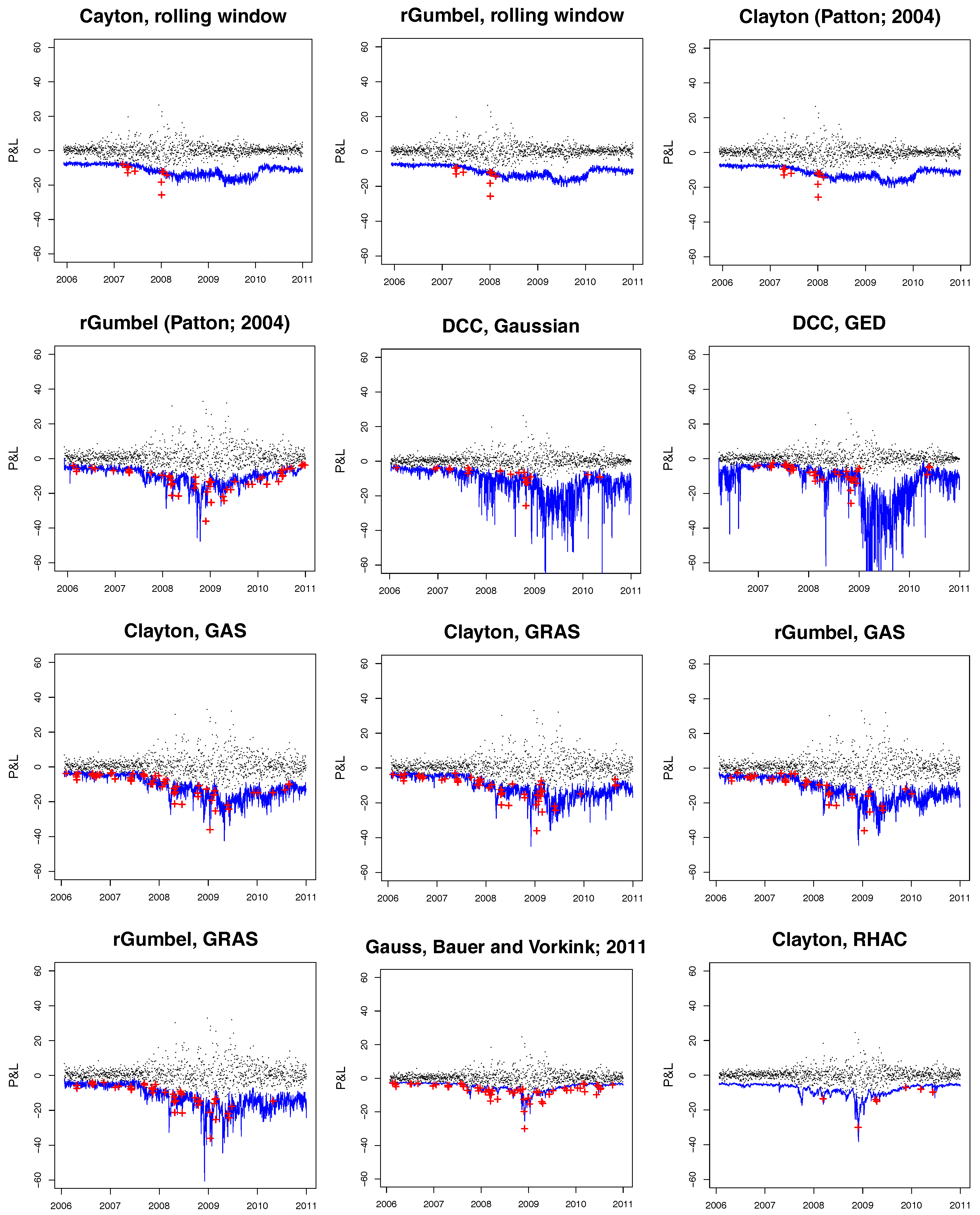
The time series of the P&L for the given portfolio and the corresponding VaR bounds are illustrated in Figure 7. The rHAC method has been found to be effective in handling the 1% and 0.5% quantiles, which is especially important in risk management. No models with a similar predictive power have been found. The hitting ratios of the dynamic copula and the realized covariance approaches are disappointing.
As was mentioned above, VaR prediction using the competing models gets computationally difficult in higher dimensions, which is not the case for the rHAC approach. The VaR regions of the rHAC model and the model of Bauer and Vorkink (2011) for a portfolio consisting of 17 assets (AA (Alcoa Inc.), AXP (American Express), BAX (Baxter International Inc.), C (Citigroup Inc.), DOW (Dow Chemical Company), GS (Goldman Sachs Group), HAS (Hasbro Inc.), HOG (Harley-Davidson Inc.), INTC (Intel Corporation), KO (Coca-Cola Co.), MET (Metlife Inc.), MSFT (Microsoft Corporation), NKE (Nike Inc.), PFE (Pfizer), VZ (Verizon Communications), XOM (Exxon Mobil Corporation) are given in Figure 8. The p-values for three considered backtesting procedures can be found in Table 4. It is evident that the multidimensional realized copula model does not suffer from the curse of dimensionality, and performs satisfactorily in the sense of unconditional coverage for moderate levels in higher dimensions. The null hypothesis of the unconditional coverage test for the Gaussian model of Bauer and Vorkink (2011) is rejected at all VaR levels.
7. Conclusions
The concept of the realized hierarchical Archimedean copula has been introduced. This model allows combining the flexibility of copula models with the additional information contained in high-frequency data. It has been suggested to combine the estimation procedures described in Segers and Uyttendaele (2014) and Górecki et al. (2016a) and adapt them to high-frequency data. This estimator is of particular importance in short-term financial risk management, as the structure and the parameters of the copula are estimated daily based solely on the realized correlation matrix.
Based on the simulation results, it has been concluded that the linear correlation matrix based estimator performs well for large enough samples; it is unbiased but less efficient that the full maximum likelihood estimator. However, it is less computationally intensive than benchmark models and does not suffer from the curse of dimensionality.
In the empirical part of the study, the proposed estimator has been applied to predict the VaR based on high-frequency data for two portfolios, one of 6 and the other of 17 assets. The results have been compared to the benchmark approaches including dynamic copulas and realized covariance models. Based on three tests (Kupiec, Christoffersen, DQ), it has been concluded that the VaR regions obtained by the high-dimensional realized copula models outperform the benchmark models in higher dimensions, especially for lower VaR levels.
Acknowledgments
We gratefully acknowledge the constructive comments of the anonymous Referees and the Editor which were helpful to revise and to improve our manuscript. We are grateful to all participants of Salzburg Workshop on Dependence Models & Copulas for the valuable suggestions and discussions. We also thank Professor Francesco Audrino and Professor Matthias Fengler, who gave us much valuable advice in the early stages of this work.
Author Contributions
Both authors contributed equally to the paper.
Conflicts of Interest
The authors declare no conflicts of interest.
Appendix A. The Generators and the Densities of Some ACs

Table A1.
Archimedean copulae: Gumbel, Clayton and Frank.
| Copula | Generator | Distribution | Parameter |
|---|---|---|---|
| Gumbel | |||
| Clayton | |||
| Frank |
Appendix B. Realized Covariance and Realized Kernel Estimator
Assume that the d-dimensional log-price process follows a Brownian semimartingale
where is a period corresponding to one trading day, is a càdlàg volatility matrix process and is a d-dimensional vector of independent Brownian motions. It is important to note that the price process is superimposed by the market microstructure noise , i.e., one observes
where , , and for . The realized covariance over the time interval is defined as the sample analog of the quadratic variation of X given by
with and is denoted by in Section 2.
One of the estimators which reduces the effect of microstructure noise is the realized kernel estimator proposed by Barndorff-Nielsen et al. (2008). As the realized covariances are obtained by summing all the cross products of log-returns that have a non zero overlapping of their respective time span, the data should be synchronized first. The procedure which is called refresh time sampling and described in Hautsch (2011) is applied to synchronize the data. The first refresh time is defined as and , where is the number of price observations for asset j. As a result, a new high-frequency vector of returns is produced, where , and n is the number of the synchronized observations.
The multivariate realized kernel estimator is given by
where is the autocovariance matrix defined as
and is the Parzen kernel
Appendix C. Simulation Results
Table A2.
Simulation results for the Gumbel copula with the structure and .
| n | |||||||
|---|---|---|---|---|---|---|---|
| CE | 30 | 0.290 | 0.391 | 0.037 | 0.254 | 0.358 | 0.492 |
| 50 | 0.377 | 0.247 | 0.014 | 0.169 | 0.222 | 0.313 | |
| 70 | 0.493 | 0.215 | 0.013 | 0.131 | 0.203 | 0.268 | |
| 100 | 0.552 | 0.183 | 0.008 | 0.116 | 0.159 | 0.235 | |
| 200 | 0.707 | 0.117 | 0.003 | 0.073 | 0.110 | 0.153 | |
| 300 | 0.784 | 0.099 | 0.002 | 0.069 | 0.088 | 0.124 | |
| 500 | 0.844 | 0.072 | 0.001 | 0.047 | 0.064 | 0.095 | |
| 800 | 0.897 | 0.063 | 0.001 | 0.042 | 0.059 | 0.081 | |
| 1000 | 0.881 | 0.053 | 0.001 | 0.031 | 0.046 | 0.068 | |
| CE | 30 | 0.251 | 0.372 | 0.041 | 0.245 | 0.319 | 0.475 |
| 50 | 0.401 | 0.234 | 0.013 | 0.152 | 0.219 | 0.297 | |
| 70 | 0.404 | 0.219 | 0.010 | 0.139 | 0.210 | 0.272 | |
| 100 | 0.463 | 0.178 | 0.007 | 0.111 | 0.169 | 0.240 | |
| 200 | 0.571 | 0.123 | 0.004 | 0.082 | 0.110 | 0.161 | |
| 300 | 0.633 | 0.101 | 0.002 | 0.070 | 0.096 | 0.124 | |
| 500 | 0.651 | 0.071 | 0.001 | 0.047 | 0.067 | 0.090 | |
| 800 | 0.714 | 0.062 | 0.001 | 0.043 | 0.061 | 0.077 | |
| 1000 | 0.707 | 0.054 | 0.001 | 0.033 | 0.048 | 0.069 | |
| SU | 30 | 0.247 | 0.368 | 0.034 | 0.233 | 0.348 | 0.467 |
| 50 | 0.292 | 0.259 | 0.018 | 0.172 | 0.241 | 0.316 | |
| 70 | 0.412 | 0.221 | 0.014 | 0.138 | 0.206 | 0.275 | |
| 100 | 0.410 | 0.175 | 0.007 | 0.117 | 0.158 | 0.219 | |
| 200 | 0.604 | 0.127 | 0.003 | 0.088 | 0.118 | 0.159 | |
| 300 | 0.680 | 0.098 | 0.002 | 0.068 | 0.087 | 0.122 | |
| 500 | 0.820 | 0.074 | 0.001 | 0.047 | 0.068 | 0.096 | |
| 800 | 0.877 | 0.061 | 0.001 | 0.041 | 0.057 | 0.078 | |
| OOS | 30 | 0.160 | 0.218 | 0.015 | 0.142 | 0.192 | 0.256 |
| 50 | 0.284 | 0.179 | 0.006 | 0.129 | 0.175 | 0.216 | |
| 70 | 0.428 | 0.143 | 0.005 | 0.093 | 0.135 | 0.175 | |
| 100 | 0.526 | 0.125 | 0.004 | 0.077 | 0.116 | 0.159 | |
| 200 | 0.743 | 0.090 | 0.002 | 0.059 | 0.085 | 0.112 | |
| 300 | 0.855 | 0.075 | 0.001 | 0.050 | 0.070 | 0.093 | |
| 500 | 0.960 | 0.059 | 0.001 | 0.038 | 0.056 | 0.076 | |
| 800 | 0.997 | 0.045 | 0.000 | 0.028 | 0.044 | 0.059 | |
| 1000 | 1.000 | 0.042 | 0.000 | 0.027 | 0.039 | 0.054 |
Table A3.
Simulation results for the Frank copula with the structure and .
| n | |||||||
|---|---|---|---|---|---|---|---|
| CE | 30 | 0.325 | 1.843 | 0.681 | 1.211 | 1.799 | 2.260 |
| 50 | 0.394 | 1.343 | 0.431 | 0.879 | 1.260 | 1.722 | |
| 70 | 0.503 | 1.176 | 0.231 | 0.852 | 1.077 | 1.440 | |
| 100 | 0.513 | 0.893 | 0.127 | 0.641 | 0.840 | 1.107 | |
| 200 | 0.714 | 0.636 | 0.080 | 0.453 | 0.597 | 0.749 | |
| 300 | 0.772 | 0.500 | 0.052 | 0.327 | 0.458 | 0.664 | |
| 500 | 0.866 | 0.405 | 0.031 | 0.264 | 0.388 | 0.524 | |
| 800 | 0.893 | 0.305 | 0.019 | 0.217 | 0.289 | 0.393 | |
| 1000 | 0.909 | 0.267 | 0.013 | 0.187 | 0.254 | 0.331 | |
| CE | 30 | 0.264 | 2.564 | 2.372 | 1.420 | 2.081 | 3.888 |
| 50 | 0.403 | 1.800 | 1.661 | 0.943 | 1.384 | 2.176 | |
| 70 | 0.430 | 1.306 | 0.824 | 0.777 | 1.104 | 1.473 | |
| 100 | 0.423 | 0.996 | 0.437 | 0.652 | 0.913 | 1.177 | |
| 200 | 0.557 | 0.628 | 0.082 | 0.414 | 0.579 | 0.813 | |
| 300 | 0.637 | 0.532 | 0.049 | 0.361 | 0.524 | 0.663 | |
| 500 | 0.685 | 0.415 | 0.034 | 0.284 | 0.392 | 0.513 | |
| 800 | 0.667 | 0.324 | 0.021 | 0.220 | 0.310 | 0.416 | |
| 1000 | 0.709 | 0.295 | 0.016 | 0.207 | 0.286 | 0.379 | |
| SU | 30 | 0.222 | 1.812 | 0.737 | 1.150 | 1.678 | 2.279 |
| 50 | 0.272 | 1.399 | 0.422 | 0.934 | 1.355 | 1.758 | |
| 70 | 0.401 | 1.140 | 0.256 | 0.787 | 1.062 | 1.433 | |
| 100 | 0.425 | 0.886 | 0.147 | 0.593 | 0.830 | 1.111 | |
| 200 | 0.601 | 0.661 | 0.079 | 0.479 | 0.633 | 0.790 | |
| 300 | 0.662 | 0.502 | 0.050 | 0.336 | 0.474 | 0.653 | |
| 500 | 0.813 | 0.399 | 0.033 | 0.256 | 0.375 | 0.522 | |
| 800 | 0.905 | 0.304 | 0.019 | 0.214 | 0.294 | 0.385 | |
| 1000 | 0.917 | 0.268 | 0.013 | 0.185 | 0.255 | 0.331 | |
| OOS | 30 | 0.186 | 1.249 | 0.343 | 0.853 | 1.152 | 1.472 |
| 50 | 0.296 | 1.028 | 0.234 | 0.752 | 0.942 | 1.273 | |
| 70 | 0.442 | 0.891 | 0.149 | 0.595 | 0.846 | 1.135 | |
| 100 | 0.524 | 0.707 | 0.096 | 0.486 | 0.651 | 0.885 | |
| 200 | 0.828 | 0.548 | 0.054 | 0.363 | 0.529 | 0.699 | |
| 300 | 0.905 | 0.453 | 0.042 | 0.303 | 0.448 | 0.574 | |
| 500 | 0.985 | 0.362 | 0.025 | 0.259 | 0.353 | 0.473 | |
| 800 | 1.000 | 0.289 | 0.017 | 0.198 | 0.266 | 0.371 | |
| 1000 | 1.000 | 0.255 | 0.013 | 0.168 | 0.249 | 0.328 |
Table A4.
Simulation results for the Gumbel copula with the structure and .
| n | |||||||
|---|---|---|---|---|---|---|---|
| CE | 30 | 0.335 | 0.521 | 0.087 | 0.320 | 0.466 | 0.614 |
| 50 | 0.398 | 0.363 | 0.023 | 0.264 | 0.336 | 0.445 | |
| 70 | 0.493 | 0.313 | 0.026 | 0.192 | 0.287 | 0.392 | |
| 100 | 0.557 | 0.270 | 0.015 | 0.188 | 0.256 | 0.325 | |
| 200 | 0.772 | 0.172 | 0.005 | 0.117 | 0.160 | 0.217 | |
| 300 | 0.885 | 0.144 | 0.004 | 0.095 | 0.133 | 0.182 | |
| 500 | 0.990 | 0.105 | 0.003 | 0.070 | 0.097 | 0.130 | |
| 800 | 1.000 | 0.086 | 0.001 | 0.062 | 0.078 | 0.105 | |
| 1000 | 1.000 | 0.079 | 0.001 | 0.052 | 0.074 | 0.099 | |
| CE | 30 | 0.345 | 0.481 | 0.091 | 0.300 | 0.408 | 0.587 |
| 50 | 0.427 | 0.358 | 0.030 | 0.238 | 0.321 | 0.441 | |
| 70 | 0.475 | 0.315 | 0.029 | 0.189 | 0.277 | 0.403 | |
| 100 | 0.581 | 0.276 | 0.016 | 0.187 | 0.259 | 0.324 | |
| 200 | 0.781 | 0.168 | 0.005 | 0.117 | 0.152 | 0.218 | |
| 300 | 0.881 | 0.143 | 0.005 | 0.097 | 0.127 | 0.173 | |
| 500 | 0.990 | 0.106 | 0.002 | 0.069 | 0.100 | 0.128 | |
| 800 | 1.000 | 0.087 | 0.002 | 0.060 | 0.077 | 0.103 | |
| 1000 | 1.000 | 0.080 | 0.001 | 0.052 | 0.077 | 0.103 | |
| SU | 30 | 0.255 | 0.536 | 0.086 | 0.322 | 0.458 | 0.622 |
| 50 | 0.290 | 0.367 | 0.029 | 0.258 | 0.341 | 0.452 | |
| 70 | 0.402 | 0.326 | 0.027 | 0.220 | 0.306 | 0.377 | |
| 100 | 0.418 | 0.274 | 0.016 | 0.185 | 0.251 | 0.329 | |
| 200 | 0.631 | 0.173 | 0.005 | 0.123 | 0.162 | 0.218 | |
| 300 | 0.697 | 0.140 | 0.004 | 0.094 | 0.128 | 0.173 | |
| 500 | 0.885 | 0.105 | 0.003 | 0.068 | 0.096 | 0.131 | |
| 800 | 0.990 | 0.086 | 0.001 | 0.062 | 0.078 | 0.105 | |
| 1000 | 0.990 | 0.078 | 0.001 | 0.051 | 0.074 | 0.098 | |
| OOS | 30 | 0.291 | 0.333 | 0.038 | 0.188 | 0.280 | 0.427 |
| 50 | 0.356 | 0.235 | 0.017 | 0.146 | 0.202 | 0.304 | |
| 70 | 0.512 | 0.219 | 0.014 | 0.138 | 0.189 | 0.264 | |
| 100 | 0.552 | 0.170 | 0.007 | 0.108 | 0.153 | 0.210 | |
| 200 | 0.772 | 0.128 | 0.003 | 0.087 | 0.122 | 0.156 | |
| 300 | 0.863 | 0.106 | 0.002 | 0.072 | 0.101 | 0.134 | |
| 500 | 0.953 | 0.086 | 0.001 | 0.059 | 0.080 | 0.106 | |
| 800 | 0.983 | 0.068 | 0.001 | 0.048 | 0.067 | 0.084 | |
| 1000 | 0.993 | 0.062 | 0.001 | 0.042 | 0.061 | 0.079 |
Table A5.
Simulation results for the Frank copula with the structure and .
| n | |||||||
|---|---|---|---|---|---|---|---|
| CE | 30 | 0.324 | 2.466 | 1.389 | 1.648 | 2.253 | 2.975 |
| 50 | 0.400 | 1.842 | 0.529 | 1.293 | 1.754 | 2.335 | |
| 70 | 0.459 | 1.542 | 0.398 | 1.106 | 1.404 | 1.950 | |
| 100 | 0.536 | 1.174 | 0.222 | 0.877 | 1.117 | 1.407 | |
| 200 | 0.749 | 0.861 | 0.101 | 0.651 | 0.829 | 1.048 | |
| 300 | 0.881 | 0.649 | 0.059 | 0.467 | 0.652 | 0.803 | |
| 500 | 1.000 | 0.529 | 0.043 | 0.379 | 0.505 | 0.637 | |
| 800 | 1.000 | 0.421 | 0.024 | 0.308 | 0.404 | 0.502 | |
| 1000 | 1.000 | 0.354 | 0.023 | 0.244 | 0.335 | 0.442 | |
| CE | 30 | 0.344 | 3.009 | 2.284 | 1.870 | 2.690 | 3.931 |
| 50 | 0.403 | 2.214 | 1.594 | 1.424 | 1.867 | 2.523 | |
| 70 | 0.451 | 1.723 | 0.872 | 1.086 | 1.528 | 2.116 | |
| 100 | 0.625 | 1.321 | 0.457 | 0.944 | 1.240 | 1.561 | |
| 200 | 0.800 | 0.944 | 0.122 | 0.697 | 0.887 | 1.169 | |
| 300 | 0.909 | 0.694 | 0.076 | 0.499 | 0.673 | 0.837 | |
| 500 | 1.000 | 0.559 | 0.053 | 0.405 | 0.537 | 0.675 | |
| 800 | 1.000 | 0.434 | 0.028 | 0.319 | 0.416 | 0.522 | |
| 1000 | 1.000 | 0.384 | 0.023 | 0.267 | 0.361 | 0.477 | |
| SU | 30 | 0.226 | 2.539 | 1.191 | 1.792 | 2.368 | 2.896 |
| 50 | 0.273 | 1.863 | 0.617 | 1.292 | 1.767 | 2.330 | |
| 70 | 0.400 | 1.635 | 0.489 | 1.153 | 1.494 | 2.031 | |
| 100 | 0.401 | 1.253 | 0.215 | 0.946 | 1.214 | 1.499 | |
| 200 | 0.606 | 0.877 | 0.107 | 0.648 | 0.846 | 1.055 | |
| 300 | 0.719 | 0.665 | 0.065 | 0.466 | 0.668 | 0.814 | |
| 500 | 0.909 | 0.514 | 0.042 | 0.362 | 0.497 | 0.619 | |
| 800 | 0.995 | 0.420 | 0.024 | 0.308 | 0.404 | 0.502 | |
| 1000 | 0.995 | 0.353 | 0.023 | 0.244 | 0.335 | 0.439 | |
| OOS | 30 | 0.261 | 1.829 | 1.017 | 1.188 | 1.582 | 2.216 |
| 50 | 0.374 | 1.357 | 0.440 | 0.838 | 1.226 | 1.666 | |
| 70 | 0.468 | 1.203 | 0.326 | 0.775 | 1.136 | 1.464 | |
| 100 | 0.580 | 0.932 | 0.163 | 0.631 | 0.884 | 1.163 | |
| 200 | 0.802 | 0.720 | 0.085 | 0.530 | 0.702 | 0.889 | |
| 300 | 0.890 | 0.596 | 0.053 | 0.442 | 0.570 | 0.723 | |
| 500 | 0.953 | 0.462 | 0.032 | 0.340 | 0.434 | 0.573 | |
| 800 | 0.983 | 0.389 | 0.021 | 0.284 | 0.372 | 0.471 | |
| 1000 | 0.990 | 0.337 | 0.020 | 0.226 | 0.324 | 0.431 |
Appendix D. Realized Volatilities and Correlations
Figure A1.
Time series of the selected daily realized volatilities (lines) and their one-day-ahead out-of-sample predictions (bold black).
Figure A1.
Time series of the selected daily realized volatilities (lines) and their one-day-ahead out-of-sample predictions (bold black).
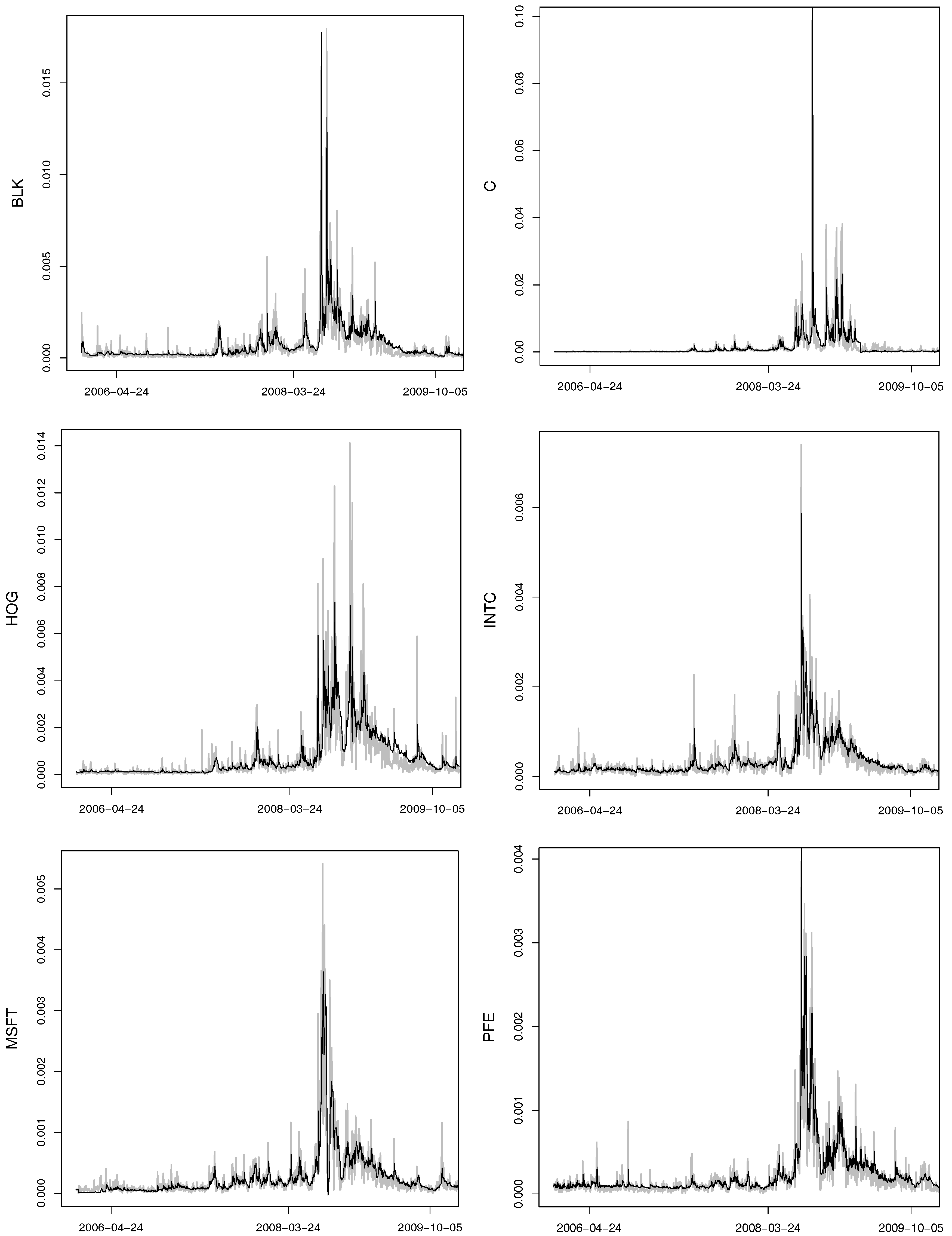
Figure A2.
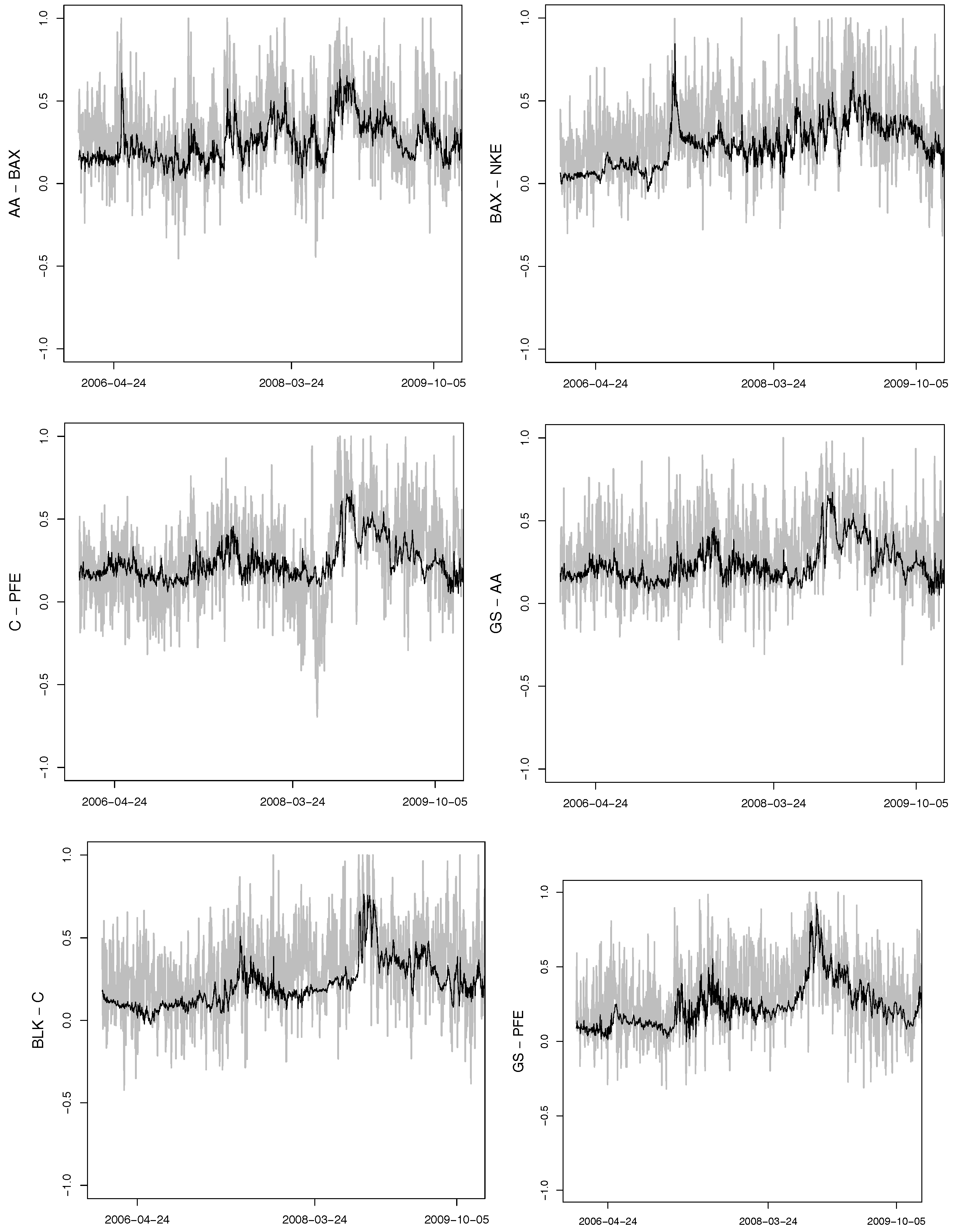
Time series of the selected daily realized correlations (grey) and their one-day-ahead out-of-sample predictions (bold black).
Figure A2.
Time series of the selected daily realized correlations (grey) and their one-day-ahead out-of-sample predictions (bold black).

Appendix E. Benchmark Models
Appendix E.1. Rolling Window Copula Model
The rolling window copula setting models the joint distribution of the standardized innovations , , via a copula with a parameter that is constant over some time period, where is the log-return and is the realized volatility of the ith asset at day t. In this study, the Clayton copula with a rolling window of days is applied. For the generalization of this approach, we refer to the locally adaptive change point algorithm of Härdle et al. (2013). This model is more flexible due to the time-varying rolling window. However, this model falls outside of the scope of this paper, due to its computational complexity.
Appendix E.2. Dynamic Copula Models
Appendix E.2.1. Copula DCC Model
Another essential class of VaR models incorporates the DCC models of Engle (2002). The mean process of the log-returns is assumed to be and the correlation of the standardized residuals , , is assumed to follow a dynamic process. These correlations are used as the input for the Student’s t copula, i.e.,
The number of degrees of freedom is kept constant, while is the conditional correlation matrix of the DCC model. In this study, we use a GJR-GARCH model for the univariate time series and DCC for the correlation of the log-returns. The normal and GED distributions are used to capture the margins .
Appendix E.2.2. The Patton (2004) Model
While in the previous setting the mean process is assumed to be , Patton (2004) suggests that the parameter of the copula should depend on a conditional mean process . This can be formalized as follows:
, , are the standardized residuals, , are unknown parameters, and the function ensures the validity of the copula parameter, for the Clayton copula and for the Gumbel copula. The marginal time series are modelled as AR-GARCH processes with GED innovations.
Appendix E.2.3. GAS and GRAS Models
Even more complex models have been proposed by Creal et al. (2013) and Salvatierra and Patton (2015). In the GAS model of Creal et al. (2013), the copula parameter follows the autoregressive process
where , is the score function of the copula of the transformed standardized residuals and is a scaling matrix. The univariate time series are assumed to be GARCH with GED margins.
The updating equation of the GRAS model of Salvatierra and Patton (2015) additionally includes the realized measure
where is the realized correlation.
Appendix E.2.4. Realized Covariance Models
The third popular class of the models are the realized covariance models. According to the methodology proposed by Bauer and Vorkink (2011), the time series of the realized covariance matrices are transformed using the matrix logarithm . Thus, the positive-definiteness of the matrix is guaranteed. In the next step, the upper-triangular elements of the matrix are stacked together in a vector , which is modeled using the HAR model. Thereafter, the vector is transformed back into the matrix . The final prediction is obtained by taking the matrix exponential, i.e., . The predicted realized covariance matrix is used as the input for a multivariate Gaussian distribution.
Another realized volatility model which uses the Cholesky decomposition instead of the logarithmic transformation is addressed in Chiriac and Voev (2011). As it performs similarly to that of Bauer and Vorkink (2011), we do not use it in the empirical part of the study.
References
- Andersen, Leif B. G., and Jakob Sidenius. 2004. Extensions to the gaussian copula: Random recovery and random factor loadings. Journal of Credit Risk 1: 29–70. [Google Scholar] [CrossRef]
- Andersen, Torben G., Tim Bollerslev, Francis X. Diebold, and Paul Labys. 2002. Modeling and forecasting realized volatility. Econometrica 71: 579–625. [Google Scholar] [CrossRef]
- Audrino, Francesco, and Fulvio Corsi. 2010. Modeling tick-by-tick realized correlations. Computational Statistics & Data Analysis 54: 2372–82. [Google Scholar]
- Barndorff-Nielsen, Ole E., Peter Reinhard Hansen, Asger Lunde, and Neil Shephard. 2004. Regular and Modified Kernel-Based Estimators of Integrated Variance: The Case with Independent Noise. University of Oslo. Available online: http://eml.berkeley.edu/~webfac/mcfadden/e242_s05/kernel.pdf (accessed on 13 June 2017).
- Barndorff-Nielsen, Ole E., Peter Reinhard Hansen, Asger Lunde, and Neil Shephard. 2008. Designing realised kernels to measure the ex-post variation of equity prices in the presence of noise. Econometrica 76: 1481–536. [Google Scholar] [CrossRef]
- Barndorff-Nielsen, Ole E., and Neil Shephard. 2004. Power and bipower variation with stochastic volatility and jumps. Journal of Financial Econometrics 2: 1–37. [Google Scholar] [CrossRef]
- Bauer, Gregory H., and Keith Vorkink. 2011. Forecasting multivariate realized stock market volatility. Journal of Econometrics 160: 93–101. [Google Scholar] [CrossRef]
- Bauwens, Luc, Giuseppe Storti, and Francesco Violante. 2012. Dynamic conditional correlation models for realized covariance matrices. CORE Discussion Paper2012060, Université catholique de Louvain, Louvain-la-Neuve, Belgium. [Google Scholar]
- Bedford, Tim, and Roger M. Cooke. 2001. Probability density decomposition for conditionally dependent random variables modeled by vines. Annals of Mathematics and Artificial Intelligence 32: 245–68. [Google Scholar] [CrossRef]
- Bollerslev, Tim, Andrew J. Pattonb, and Rogier Quaedvlieg. 2016. Modeling and forecasting (un) reliable realized covariances for more reliable financial decisions. Available online: http://public.econ.duke.edu/~ap172/BPQ_MV_HARQ_apr16.pdf (accessed on 13 June 2017).
- Breymann, Wolfgang, Alexandra Dias, and Paul Embrechts. 2003. Dependence Structures for Multivariate High-Frequency Data in Finance. Quantitative Finance 3: 1–14. [Google Scholar] [CrossRef]
- Brownless, Christian T., and Giampiero Gallo. 2006. Financial econometric analysis at ultra-high frequency: Data handling concerns. Computational Statistics & Data Analysis 51: 2232–45. [Google Scholar]
- Cherubini, Umberto, Sabrina Mulinacci, Fabio Gobbi, and Silvia Romagnoli. 2011. Dynamic Copula Methods in Finance. Hoboken: John Wiley & Sons. [Google Scholar]
- Chiriac, Roxana, and Valeri Voev. 2011. Modelling and forecasting multivariate realized volatility. Journal of Econometrics 26: 922–47. [Google Scholar] [CrossRef]
- Christoffersen, Peter, and Denis Pelletier. 2004. Backtesting value-at-risk: A duration-based approach. Journal of Financial Econometrics 2: 84–108. [Google Scholar] [CrossRef]
- Corsi, Fulvio. 2009. A simple approximate long-memory model of realized volatility. Journal of Financial Econometrics 7: 174–96. [Google Scholar] [CrossRef]
- Creal, Drew, Siem Jan Koopman, and Lucas André. 2013. Generalized autoregressive score models with applications. Journal of Applied Econometrics 28: 777–95. [Google Scholar] [CrossRef]
- Czado, Claudia. 2010. Pair-copula constructions of multivariate copulas. In Copula Theory and Its Applications. Lecture Notes in Statistics. Edited by P. Jaworski, F. Durante, W. Härdle and T. Rychlik. Berlin and Heidelberg: Springer, pp. 93–109. [Google Scholar]
- Dias, Alexandra, and Paul Embrechts. 2004. Dynamic copula models for multivariate high-frequency data in finance. Available online: http://www2.warwick.ac.uk/fac/soc/wbs/subjects/finance/research/wpaperseries/wf06-250.pdf (accessed on 13 June 2017).
- Durante, Fabrizio, and Carlo Sempi. 2015. Principles of Copula Theory. Boca Raton: Chapman and Hall. [Google Scholar]
- Embrechts, Paul, Andrea Höing, and Alessandro Juri. 2003. Using copulae to bound the value-at-risk for functions of dependent risks. Finance & Stochastics 7: 145–67. [Google Scholar]
- Embrechts, Paul, Alexander McNeil, and Daniel Straumann. 1999. Correlation: Pitfalls and alternatives. RISK 12: 69–71. [Google Scholar]
- Engle, Robert F. 2002. Dynamical conditional correlation: A simple class of multivariate generalized autoregressive conditional heteroscedastic models. Journal of Business and Economic Statistics 20, (3): 339–50. [Google Scholar] [CrossRef]
- Engle, Robert F., and Simone Manganelli. 2004. Caviar: Conditional autoregressive value at risk by regression quantiles. Journal of Business & Economic Statistics 22: 367–81. [Google Scholar]
- Fengler, Matthias R., and Ostap Okhrin. 2016. Managing risk with a realized copula parameter. Computational Statistics & Data Analysis 100: 131–52. [Google Scholar]
- Genest, Christian, Johanna Nešlehová, and Johanna Ziegel. 2011. Inference in multivariate archimedean copula models. Test 20: 223–56. [Google Scholar] [CrossRef]
- Genest, Christian, Johanna Nešlehová, and Noomen Ben Ghorbal. 2011. Estimators based on kendall’s tau in multivariate copula models. Australian and New Zealand Journal of Statistics 53: 157–77. [Google Scholar] [CrossRef]
- Górecki, Jan, Marius Hofert, and Martin Holeňa. 2014. On the consistency of an estimator for hierarchical archimedean copulas. Paper presented at 32nd International Conference on Mathematical Methods in Economics, Olomouc, Czech Republic, 10–12 September; pp. 239–44. [Google Scholar]
- Górecki, Jan, Marius Hofert, and Martin Holeňa. 2016a. An approach to structure determination and estimation of hierarchical archimedean copulas and its application to bayesian classification. Journal of Intelligent Information Systems 46: 21–59. [Google Scholar] [CrossRef]
- Górecki, Jan, Marius Hofert, and Martin Holeňa. 2016b. On structure, family and parameter estimation of hierarchical archimedean copulas. arXiv. [Google Scholar]
- Hansen, Peter Reinhard, Asger Lunde, and Voev Valeri. 2014. Realized beta garch: A multivariate garch model with realized measures of volatility. Journal of Applied Econometrics 29: 774–99. [Google Scholar] [CrossRef]
- Härdle, Wolfgang Karl, Okhrin Ostap, and Okhrin Yarema. 2013. Dynamic structured copula models. Statistics & Risk Modeling 30: 361–88. [Google Scholar]
- Hastie, Trevor, Robert Tibshirani, and Jerome Friedman. 2009. The Elements of Statistical Learning Data Mining, Inference, and Prediction. New York: Springer. [Google Scholar]
- Hautsch, Nikolaus. 2011. Econometrics of Financial High-Frequency Data. Berlin and Heidelberg: Springer Science & Business Media. [Google Scholar]
- Hayashi, Takaki, and Nakahiro Yoshida. 2005. On covariance estimation of non-synchronously observed diffusion processes. Bernoulli 11: 359–79. [Google Scholar] [CrossRef]
- Hoeffding, Wassily. 1940. Scale-invariant correlation theory. Schriften des Mathematischen Instituts und des Instituts fur Angewandte Mathematik der Universit at Berlin 5: 181–233. [Google Scholar]
- Hofert, Marius, and Matthias Scherer. 2011. Cdo pricing with nested archimedean copulas. Quantitative Finance 11: 775–87. [Google Scholar] [CrossRef]
- Jaworski, Piotr, Fabrizio Durante, and Wolfgang Karl Härdle. 2013. Copulae in Mathematical and Quantitative Finance. Berlin and Heidelberg: Springer. [Google Scholar]
- Jin, Xin, and John M. Maheu. 2012. Modeling realized covariances and returns. Journal of Financial Econometrics 11: 335–69. [Google Scholar] [CrossRef]
- Joe, Harry. 1996. Families of m-variate distributions with given margins and m(m-1)/2 bivariate dependence parameters. IMS Lecture Notes 28: 120–41. [Google Scholar]
- Joe, Harry. 2014. Dependence Modeling with Copulas. Boca Raton: CRC Press. [Google Scholar]
- Kaufman, Leonard, and Peter J. Rousseeuw. 2005. Finding Groups in Data: An Introduction to Cluster Analysis. New York: Wiley. [Google Scholar]
- Krämer, Nicole, Eike C. Brechmann, Daniel Silvestrini, and Claudia Czado. 2013. Total loss estimation using copula-based regression models. Insurance: Mathematics and Economics 53: 829–39. [Google Scholar] [CrossRef]
- Krupskii, Pavel, and Harry Joe. 2013. Factor copula models for multivariate data. Journal of Multivariate Analysis 120: 85–101. [Google Scholar] [CrossRef]
- Kupiec, Paul H. 1995. Techniques for verifying the accuracy of risk measurement models. The Jouranl of Derivatives 3: 73–84. [Google Scholar] [CrossRef]
- Kurowicka, Dorota. 2011. Dependence Modeling: Vine Copula Handbook. Singapore: World Scientific. [Google Scholar]
- Nelsen, Roger B. 1996. Nonparametric Measures of Multivariate Association. Lecture Notes-Monograph Series 28: 223–32. [Google Scholar]
- Nelsen, Roger B. 2007. An Introduction to Copulas. New York: Springer Science & Business Media. [Google Scholar]
- Noureldin, Diaa, Neil Shephard, and Kevin Sheppard. 2012. Multivariate high-frequency-based volatility (heavy) models. Journal of Applied Econometrics 27: 907–33. [Google Scholar] [CrossRef]
- Oh, Dong Hwan, and Andrew J. Patton. 2017. Modeling dependence in high dimensions with factor copulas. Journal of Business & Economic Statistics 35: 139–54. [Google Scholar]
- Okhrin, Ostap, Yarema Okhrinb, and Wolfgang Schmidc. 2013. On the structure and estimation of hierarchical archimedean copulas. Journal of Econometrics 173: 189–204. [Google Scholar] [CrossRef]
- Okhrin, Ostap, and Alexander Ristig. 2014. Hierarchical archimedean copulae: The hac package. Journal of Statistical Software 58, Issue 4. [Google Scholar]
- Okhrin, Ostap, Alexander Ristig, Jeffrey Sheen, and Stefan Trück. 2015. Conditional Systemic Risk with Penalized Copula. SFB 649 Discussion Paper SFB649DP2015-038, Sonderforschungsbereich 649, Humboldt University, Berlin, Germany. [Google Scholar]
- Patton, Andrew J. 2004. On the out-of-sample importance of skewness and asymmetric dependence for asset allocation. Journal of Financial Econometrics 2: 130–68. [Google Scholar] [CrossRef]
- De Pooter, Michiel, Martin Martens, and Dick van Dijk. 2008. Predicting the daily covariance matrix for s & p 100 stocks using intraday data—But which frequency to use? Econometric Reviews 27: 199–229. [Google Scholar]
- Rodriguez, Juan Carlos. 2007. Measuring financial contagition: A copula approach. Journal of Empirical Finance 3: 401–23. [Google Scholar] [CrossRef]
- De Lira Salvatierra, Irving Arturo, and Andrew J. Patton. 2015. Dynamic copula models and high frequency data. Journal of Empirical Finance 30: 120–35. [Google Scholar] [CrossRef]
- Segers, Johan, and Nathan Uyttendaele. 2014. Nonparametric estimation of the tree structure of a nested archimedean copula. Computational Statistics & Data Analysis 72: 190–204. [Google Scholar]
- Sklar, M. 1959. Functions de Repartition A N Dimensionset Leurs Marges. Paris: Inst. Statis. Univ. Paris, No. 8. [Google Scholar]
- Trivedi, Pravin K., and David M. Zimmer. 2007. Copula Modeling: An Introduction for Practitioners. Boston, Delft: Now Publishers, Inc., vol. 1. [Google Scholar]
- Uyttendaele, Nathan. 2016. On the Estimation of Nested Archimedean Copulas: A Theoretical and an Experimental Comparison. Available online: http://dial.uclouvain.be/pr/boreal/en/object/boreal%3A171500/datastreams (accessed on 13 June 2017).
- Van der Voort, Martijn. 2007. Factor copulas: External defaults. The Journal of Derivatives 14: 94–102. [Google Scholar] [CrossRef]
- Zhang, Lan, Per A. Mykland, and Yacine Aït-Sahalia. 2005. A tale of two time scales: Determining integrated volatility with noisy high-frequency data. Journal of the American Statistical Association 100: 1394–411. [Google Scholar] [CrossRef]
Figure 1.
A 5-dimensional copula structure.

Figure 2.
A set of trivariate structures corresponding to the copula with .

Figure 3.
Dendrograms for the trivial Gumbel copula , the binary Gumbel copula (center) and kernel density estimate of , where , blue for the trivial structure and green for the binary structure.
Figure 3.
Dendrograms for the trivial Gumbel copula , the binary Gumbel copula (center) and kernel density estimate of , where , blue for the trivial structure and green for the binary structure.
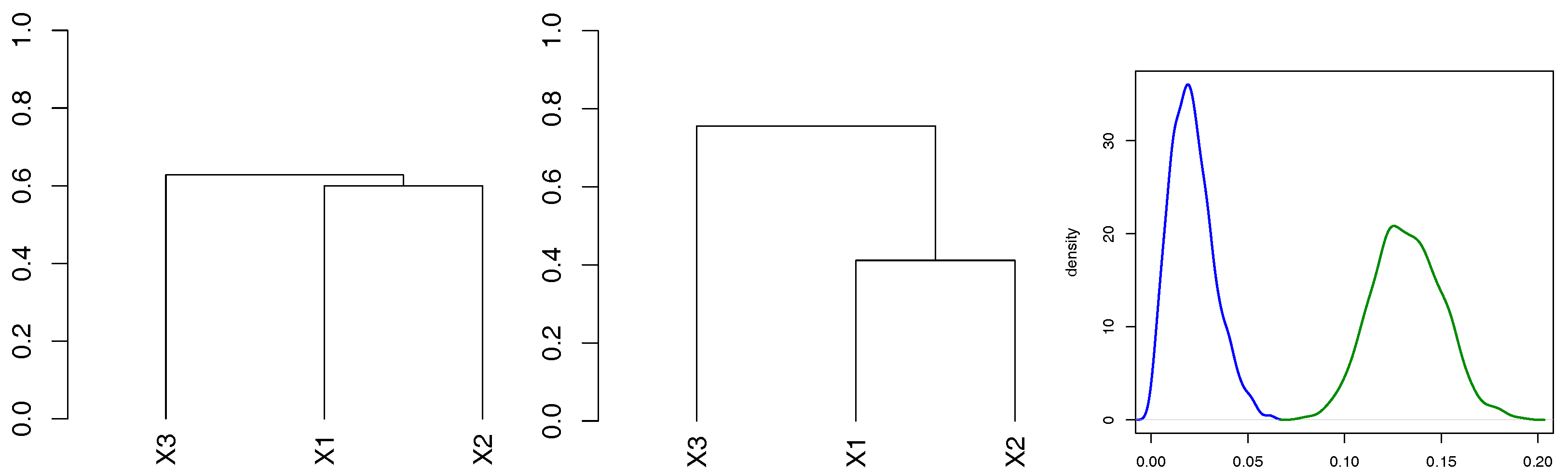
Figure 4.
Structures of the 5-dimensional copulae used in the simulation studies.

Figure 5.
KDE of (green), (red) and KDE of the Gaussian distribution sample (blue) for the Gumbel copula with the structure and .
Figure 5.
KDE of (green), (red) and KDE of the Gaussian distribution sample (blue) for the Gumbel copula with the structure and .
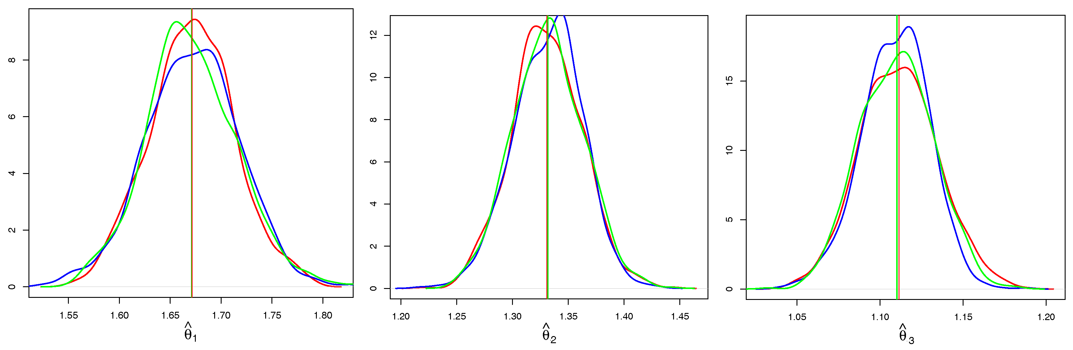
Figure 6.
Average log computational time (in seconds) over 100 simulations for the estimation of the Clayton copula by clustering estimator (CE) and the benchmark models depending on the dimension.
Figure 6.
Average log computational time (in seconds) over 100 simulations for the estimation of the Clayton copula by clustering estimator (CE) and the benchmark models depending on the dimension.
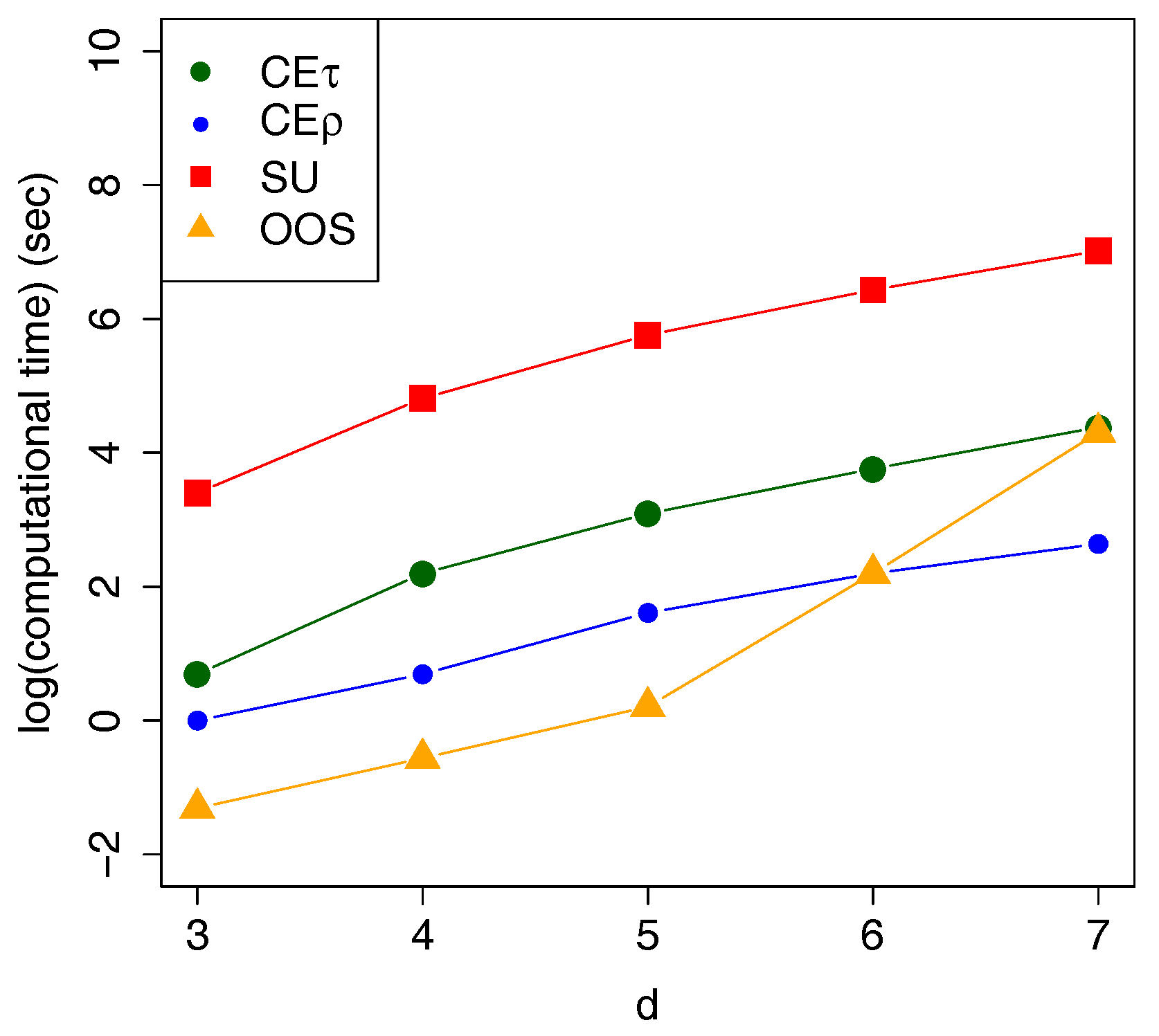
Figure 7.
Exceedances for the VaR (0.01) of the AA-AXP-BAX-C-INTC-KO portfolio. P & L (black dots), the lower VaR(0.01) (blue solid line), exceedances (red crosses).
Figure 7.
Exceedances for the VaR (0.01) of the AA-AXP-BAX-C-INTC-KO portfolio. P & L (black dots), the lower VaR(0.01) (blue solid line), exceedances (red crosses).

Figure 8.
Exceedances for the VaR(0.01) of the AA-AXP-BAX-BLK-C-DOW-GS-HAS-HOG-INTC-KO-MET-MSFT-NKE-PFE-VZ-XOM portfolio. P&L (black dots), the lower VaR(0.01) (blue solid line), exceedances (red crosses).
Figure 8.
Exceedances for the VaR(0.01) of the AA-AXP-BAX-BLK-C-DOW-GS-HAS-HOG-INTC-KO-MET-MSFT-NKE-PFE-VZ-XOM portfolio. P&L (black dots), the lower VaR(0.01) (blue solid line), exceedances (red crosses).
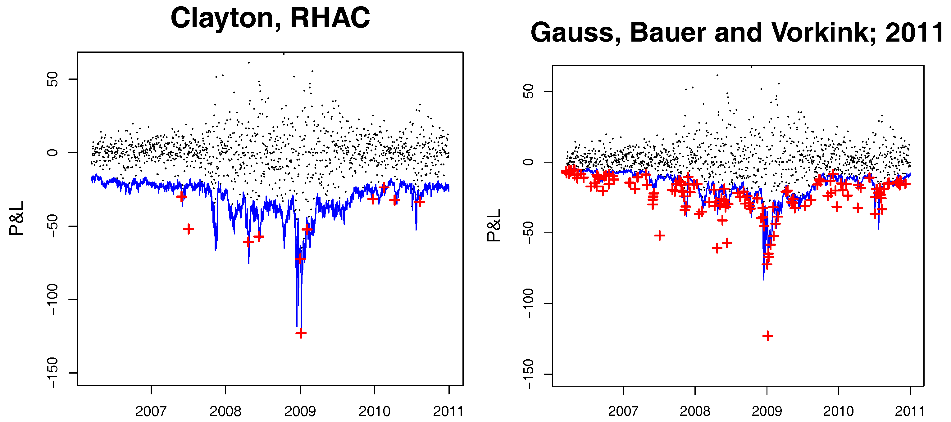
Table 1.
Simulation results for the Clayton copula with the structure and .
| n | |||||||
|---|---|---|---|---|---|---|---|
| CE | 30 | 0.262 | 0.738 | 0.175 | 0.465 | 0.686 | 0.930 |
| 50 | 0.370 | 0.518 | 0.078 | 0.312 | 0.449 | 0.650 | |
| 70 | 0.449 | 0.435 | 0.040 | 0.290 | 0.401 | 0.543 | |
| 100 | 0.570 | 0.356 | 0.023 | 0.249 | 0.338 | 0.460 | |
| 200 | 0.797 | 0.236 | 0.013 | 0.158 | 0.221 | 0.279 | |
| 300 | 0.847 | 0.190 | 0.007 | 0.126 | 0.180 | 0.241 | |
| 500 | 0.873 | 0.137 | 0.004 | 0.091 | 0.124 | 0.177 | |
| 800 | 0.905 | 0.113 | 0.003 | 0.070 | 0.107 | 0.144 | |
| 1000 | 0.840 | 0.110 | 0.003 | 0.070 | 0.097 | 0.142 | |
| CE | 30 | 0.268 | 1.716 | 3.813 | 0.525 | 0.816 | 1.519 |
| 50 | 0.439 | 1.104 | 2.468 | 0.355 | 0.556 | 0.725 | |
| 70 | 0.472 | 0.853 | 1.828 | 0.309 | 0.466 | 0.650 | |
| 100 | 0.592 | 0.483 | 0.645 | 0.242 | 0.342 | 0.461 | |
| 200 | 0.797 | 0.247 | 0.014 | 0.166 | 0.228 | 0.314 | |
| 300 | 0.866 | 0.198 | 0.008 | 0.128 | 0.181 | 0.255 | |
| 500 | 0.870 | 0.146 | 0.005 | 0.093 | 0.135 | 0.192 | |
| 800 | 0.917 | 0.115 | 0.004 | 0.067 | 0.110 | 0.155 | |
| 1000 | 0.873 | 0.115 | 0.003 | 0.070 | 0.106 | 0.153 | |
| SU | 30 | 0.203 | 0.727 | 0.136 | 0.469 | 0.679 | 0.934 |
| 50 | 0.276 | 0.532 | 0.069 | 0.336 | 0.513 | 0.663 | |
| 70 | 0.349 | 0.449 | 0.051 | 0.292 | 0.401 | 0.562 | |
| 100 | 0.441 | 0.360 | 0.024 | 0.259 | 0.336 | 0.464 | |
| 200 | 0.645 | 0.250 | 0.015 | 0.164 | 0.231 | 0.301 | |
| 300 | 0.722 | 0.188 | 0.008 | 0.123 | 0.171 | 0.239 | |
| 500 | 0.847 | 0.138 | 0.005 | 0.093 | 0.124 | 0.178 | |
| 800 | 0.905 | 0.113 | 0.003 | 0.070 | 0.107 | 0.144 | |
| 1000 | 0.840 | 0.110 | 0.003 | 0.070 | 0.097 | 0.142 | |
| OOS | 30 | 0.141 | 0.323 | 0.027 | 0.224 | 0.297 | 0.422 |
| 50 | 0.216 | 0.298 | 0.021 | 0.188 | 0.267 | 0.376 | |
| 70 | 0.300 | 0.257 | 0.014 | 0.178 | 0.240 | 0.321 | |
| 100 | 0.402 | 0.225 | 0.011 | 0.154 | 0.212 | 0.270 | |
| 200 | 0.647 | 0.154 | 0.006 | 0.093 | 0.151 | 0.194 | |
| 300 | 0.740 | 0.129 | 0.003 | 0.089 | 0.119 | 0.162 | |
| 500 | 0.915 | 0.103 | 0.002 | 0.069 | 0.099 | 0.134 | |
| 800 | 0.980 | 0.075 | 0.001 | 0.052 | 0.073 | 0.094 | |
| 1000 | 0.983 | 0.071 | 0.001 | 0.049 | 0.065 | 0.092 |
Table 2.
Simulation results for the Clayton copula with the structure and .
| n | |||||||
|---|---|---|---|---|---|---|---|
| CE | 30 | 0.288 | 1.095 | 0.551 | 0.664 | 0.954 | 1.268 |
| 50 | 0.374 | 0.766 | 0.145 | 0.480 | 0.727 | 0.966 | |
| 70 | 0.407 | 0.659 | 0.188 | 0.443 | 0.566 | 0.772 | |
| 100 | 0.601 | 0.506 | 0.050 | 0.357 | 0.485 | 0.638 | |
| 200 | 0.858 | 0.336 | 0.026 | 0.223 | 0.315 | 0.431 | |
| 300 | 0.939 | 0.288 | 0.017 | 0.192 | 0.271 | 0.361 | |
| 500 | 0.995 | 0.213 | 0.007 | 0.151 | 0.206 | 0.262 | |
| 800 | 1.000 | 0.167 | 0.005 | 0.113 | 0.153 | 0.209 | |
| 1000 | 1.000 | 0.158 | 0.004 | 0.114 | 0.148 | 0.202 | |
| CE | 30 | 0.262 | 2.352 | 3.969 | 0.830 | 1.413 | 5.358 |
| 50 | 0.421 | 1.420 | 2.553 | 0.543 | 0.838 | 1.260 | |
| 70 | 0.475 | 0.978 | 1.593 | 0.412 | 0.612 | 0.873 | |
| 100 | 0.621 | 0.687 | 0.755 | 0.364 | 0.516 | 0.713 | |
| 200 | 0.885 | 0.352 | 0.028 | 0.242 | 0.318 | 0.424 | |
| 300 | 0.952 | 0.324 | 0.022 | 0.219 | 0.292 | 0.402 | |
| 500 | 1.000 | 0.228 | 0.013 | 0.154 | 0.216 | 0.276 | |
| 800 | 1.000 | 0.183 | 0.007 | 0.121 | 0.164 | 0.220 | |
| 1000 | 1.000 | 0.169 | 0.006 | 0.110 | 0.161 | 0.210 | |
| SU | 30 | 0.252 | 1.072 | 0.329 | 0.657 | 0.959 | 1.329 |
| 50 | 0.401 | 0.756 | 0.146 | 0.464 | 0.699 | 0.926 | |
| 70 | 0.448 | 0.657 | 0.097 | 0.447 | 0.598 | 0.809 | |
| 100 | 0.401 | 0.508 | 0.050 | 0.360 | 0.471 | 0.616 | |
| 200 | 0.615 | 0.353 | 0.026 | 0.234 | 0.339 | 0.447 | |
| 300 | 0.760 | 0.300 | 0.018 | 0.194 | 0.284 | 0.369 | |
| 500 | 0.939 | 0.207 | 0.006 | 0.147 | 0.206 | 0.253 | |
| 800 | 0.995 | 0.167 | 0.005 | 0.113 | 0.153 | 0.209 | |
| 1000 | 1.000 | 0.158 | 0.004 | 0.114 | 0.148 | 0.202 | |
| OOS | 30 | 0.388 | 0.539 | 0.096 | 0.333 | 0.447 | 0.657 |
| 50 | 0.536 | 0.420 | 0.046 | 0.278 | 0.376 | 0.508 | |
| 70 | 0.666 | 0.359 | 0.024 | 0.244 | 0.328 | 0.451 | |
| 100 | 0.774 | 0.305 | 0.017 | 0.212 | 0.291 | 0.364 | |
| 200 | 0.953 | 0.226 | 0.008 | 0.165 | 0.217 | 0.271 | |
| 300 | 0.985 | 0.198 | 0.007 | 0.135 | 0.183 | 0.246 | |
| 500 | 0.998 | 0.146 | 0.004 | 0.099 | 0.137 | 0.179 | |
| 800 | 1.000 | 0.112 | 0.002 | 0.081 | 0.108 | 0.141 | |
| 1000 | 1.000 | 0.106 | 0.002 | 0.070 | 0.101 | 0.133 |
Table 3.
VaR performance for the AA-AXP-BAX-C-INTC-KO. The hitting ratio and the p-values of the Kupiec test (K), Christoffersen (C), and the dynamic quantile (DQ) test.
Table 3.
VaR performance for the AA-AXP-BAX-C-INTC-KO. The hitting ratio and the p-values of the Kupiec test (K), Christoffersen (C), and the dynamic quantile (DQ) test.
| Model | Level | K | C | DQ | |
|---|---|---|---|---|---|
| Rolling window, Clayton, GED | 0.0030 | 0.2712 | 0.0317 | 0.6756 | |
| 0.0076 | 0.3510 | 0.0000 | 0.6619 | ||
| 0.0514 | 0.8163 | 1.0000 | 0.1290 | ||
| 0.1043 | 0.0000 | 0.0000 | 0.0070 | ||
| Rolling window, rGumbel, GED | 0.0045 | 0.8076 | 0.0018 | 0.4378 | |
| 0.0083 | 0.5257 | 0.0000 | 0.0053 | ||
| 0.0506 | 0.9148 | 0.0000 | 0.0186 | ||
| 0.0990 | 0.0000 | 0.0000 | 0.0016 | ||
| DCC, t-copula | 0.0232 | 0.0001 | 0.0000 | 0.0139 | |
| 0.0304 | 0.0000 | 0.0000 | 0.0041 | ||
| 0.0728 | 0.0000 | 0.0000 | 0.0001 | ||
| 0.1112 | 0.0000 | 0.0000 | 0.0000 | ||
| DCC, t-copula, GED | 0.0054 | 0.0671 | 0.0000 | 0.9796 | |
| 0.0162 | 0.0403 | 0.0000 | 0.0000 | ||
| 0.0470 | 0.0000 | 0.0000 | 0.3045 | ||
| 0.0924 | 0.0000 | 0.0000 | 0.2985 | ||
| Patton, Clayton | 0.0509 | 0.0000 | 0.0377 | 0.6360 | |
| 0.0616 | 0.0000 | 0.0601 | 0.7315 | ||
| 0.1036 | 0.0000 | 0.2041 | 0.7414 | ||
| 0.1366 | 0.0001 | 0.3031 | 0.4549 | ||
| Patton, rGumbel | 0.0332 | 0.0000 | 0.0786 | 0.8460 | |
| 0.0370 | 0.0000 | 0.0425 | 0.6558 | ||
| 0.0612 | 0.0709 | 0.0653 | 0.5654 | ||
| 0.0937 | 0.4372 | 0.1178 | 0.3615 | ||
| GAS, Clayton, GED | 0.0303 | 0.0000 | 0.0549 | 0.0726 | |
| 0.0427 | 0.0000 | 0.0079 | 0.1935 | ||
| 0.0822 | 0.0000 | 0.0493 | 0.0078 | ||
| 0.1404 | 0.0000 | 0.4827 | 0.0046 | ||
| GRAS, Clayton, GED | 0.0303 | 0.0000 | 0.0002 | 0.0001 | |
| 0.0388 | 0.0000 | 0.0000 | 0.0001 | ||
| 0.0869 | 0.0000 | 0.0234 | 0.0014 | ||
| 0.1381 | 0.0000 | 0.5202 | 0.0164 | ||
| GAS, rGumbel, GED | 0.0217 | 0.0000 | 0.0208 | 0.0838 | |
| 0.0295 | 0.0000 | 0.0052 | 0.0150 | ||
| 0.0760 | 0.0001 | 0.0035 | 0.0007 | ||
| 0.1296 | 0.0007 | 1.0000 | 0.0027 | ||
| GRAS, rGumbel, GED | 0.0202 | 0.0000 | 0.0052 | 0.0884 | |
| 0.0326 | 0.0000 | 0.0001 | 0.0639 | ||
| 0.0706 | 0.0014 | 0.0242 | 0.0228 | ||
| 0.1327 | 0.0002 | 1.0000 | 0.0345 | ||
| RCov, Bauer and Vorkink | 0.0350 | 0.0000 | 0.2920 | 0.0009 | |
| 0.0474 | 0.0000 | 0.1937 | 0.0008 | ||
| 0.1213 | 0.0000 | 0.8088 | 0.0038 | ||
| 0.1773 | 0.0000 | 0.0017 | 0.0017 | ||
| rHAC, Clayton | 0.0047 | 0.8589 | 0.5042 | 0.0000 | |
| 0.0085 | 0.5873 | 0.5064 | 0.0028 | ||
| 0.0551 | 0.4098 | 0.1521 | 0.0000 | ||
| 0.1140 | 0.0995 | 0.1482 | 0.0000 |
Table 4.
VaR performance for the AA-AXP-BAX-BLK-C-DOW-GS-HAS-HOG-INTC-KO-MET-MSFT-NKE-PFE-VZ-XOM. The hitting ratio and the p-values of the Kupiec test (K), Christoffersen (C), and the DQ test.
Table 4.
VaR performance for the AA-AXP-BAX-BLK-C-DOW-GS-HAS-HOG-INTC-KO-MET-MSFT-NKE-PFE-VZ-XOM. The hitting ratio and the p-values of the Kupiec test (K), Christoffersen (C), and the DQ test.
| Model | Level | K | C | DQ | |
|---|---|---|---|---|---|
| rHAC, Clayton | 0.0040 | 0.6008 | 0.1006 | 0.0006 | |
| 0.0088 | 0.6593 | 0.5534 | 0.0000 | ||
| 0.0192 | 0.0000 | 0.3231 | 0.0000 | ||
| 0.0791 | 0.0107 | 0.6305 | 0.0000 | ||
| RCov, Bauer and Voev | 0.0799 | 0.0000 | 0.7393 | 0.9752 | |
| 0.1102 | 0.0000 | 0.7745 | 0.0710 | ||
| 0.1294 | 0.0000 | 0.3221 | 0.0582 | ||
| 0.1925 | 0.0000 | 0.0002 | 0.1289 |
© 2017 by the authors. Licensee MDPI, Basel, Switzerland. This article is an open access article distributed under the terms and conditions of the Creative Commons Attribution (CC BY) license (http://creativecommons.org/licenses/by/4.0/).
Share and Cite
MDPI and ACS Style
Okhrin, O.; Tetereva, A. The Realized Hierarchical Archimedean Copula in Risk Modelling. Econometrics 2017, 5, 26. https://doi.org/10.3390/econometrics5020026
AMA Style
Okhrin O, Tetereva A. The Realized Hierarchical Archimedean Copula in Risk Modelling. Econometrics. 2017; 5(2):26. https://doi.org/10.3390/econometrics5020026
Chicago/Turabian StyleOkhrin, Ostap, and Anastasija Tetereva. 2017. "The Realized Hierarchical Archimedean Copula in Risk Modelling" Econometrics 5, no. 2: 26. https://doi.org/10.3390/econometrics5020026
Note that from the first issue of 2016, this journal uses article numbers instead of page numbers. See further details here.