
Results of Long-Duration Simulation of Distant Retrograde Orbits

Odyssey Space Research, 1120 NASA Pkwy, Houston, TX 77058, USA
Aerospace 2016, 3(4), 37; https://doi.org/10.3390/aerospace3040037
Submission received: 31 July 2016
/
Revised: 23 October 2016
/
Accepted: 26 October 2016
/
Published: 8 November 2016
Abstract
:Distant Retrograde Orbits in the Earth–Moon system are gaining in popularity as stable “parking” orbits for various conceptual missions. To investigate the stability of potential Distant Retrograde Orbits, simulations were executed, with propagation running over a thirty-year period. Initial conditions for the vehicle state were limited such that the position and velocity vectors were in the Earth–Moon orbital plane, with the velocity oriented such that it would produce retrograde motion about Moon. The resulting trajectories were investigated for stability in an environment that included the eccentric motion of Moon, non-spherical gravity of Earth and Moon, gravitational perturbations from Sun, Jupiter, and Venus, and the effects of radiation pressure. The results indicate that stability may be enhanced at certain resonant states within the Earth–Moon system.

1. Introduction
1.1. Overview
The term Distant Retrograde Orbit (DRO) was introduced by O’Campo and Rosborough [1] to describe a set of trajectories that appeared to orbit the Earth–Moon system in a retrograde sense when compared with the motion of the Earth/Moon around the solar-system barycenter. It has since been extended to be a generic term applied to the motion of a minor body around the three-body system-barycenter where such motion gives the appearance of retrograde motion about the secondary body in the system. Of particular interest to mission planners are the trajectories of a vehicle in retrograde motion about Moon when viewed from the Earth–Moon barycenter.
The stability of the retrograde solution to the Hill problem (plane-restricted three-body problem where the mass of the second body is small) was earlier investigated by Hénon [2], with the conclusion that stable retrograde trajectories are theoretically possible at all radii in such a system. However, there are significant complications inherent in the real n-body problem representing a vehicle in the Earth–Moon system: the large and irregular second-body mass (Moon) provides a significant gravitational perturbation; in-plane perturbations from tertiary bodies (e.g., Sun, Jupiter) void the 3-body assumption of the Hill problem; and out-of-plane perturbations from the same void the assumption of plane-restricted dynamics. Perturbations from Sun will typically be dominated by gravity, but solar radiation pressure may also be influential.
The theoretical long-duration stability feature of DROs has led to the recent consideration of DRO trajectories for several mission concepts, mostly in the Earth–Moon system; the most publicized of these is probably NASA’s Asteroid Retrieval Mission, but others—such as using DRO for Earth–Mars transfers [3]—are also available in the public realm. The current state of understanding of the long-term stability of such orbits adds significant and unnecessary risk to such mission concepts. Because most of these potential missions are in the Earth–Moon system, that is the most urgent system to consider for identification of stable conditions. Thus, the analyses presented herein focus exclusively on retrograde orbits around Moon.
This paper focuses on the identification of initial conditions that give rise to DRO trajectories that are stable over the lifetime of a typical program; thirty years was selected as a conservative term for most projects. In this context, the term stable is used to identify those conditions that lead to orbits that are still in the Earth–Moon system after propagating for thirty years. The characterization of the final state of those initial conditions is not explored exhaustively, although the regularity of certain trajectories—particularly resonant trajectories—suggest that most, if not all, stable DROs maintain a fairly regular characteristic state.
This identification of initial conditions for stable lunar orbits can be used to provide suitable target conditions for mission-planning purposes. The methods for reaching those target conditions are not covered in this paper. Simple direct-injection techniques result in required delta-V values of approximately 3 km·s for departure from Low Earth Orbit (LEO) onto a transfer orbit, plus approximately 1 km·s for injection into the DRO. These baseline delta-V values can be reduced by utilizing more elaborate transfers [4,5,6].
This paper does not attempt to demonstrate why some conditions lead to stable orbits while others do not, nor discover the ultimate causes of the instabilities for those conditions that fail to reach thirty years. Such work has been investigated before; Bezrouk and Parker [7] demonstrated the modes by which a small selection of DRO orbits may become unstable, and identified solar gravity as the leading source of instability for those orbits. Characterization of out-of-plane initial conditions that also lead to stable trajectories is left for future work. This paper also limits the analysis to the energetically-favorable in-plane initial conditions, with acknowledgment that:
- there are likely additional stable conditions with motion out of the Earth–Moon orbital plane, and
- while the initial conditions are co-planar with the Earth–Moon orbital plane, it is unlikely that such conditions would produce motion that remains exclusively in that plane for the duration of the simulation.
The additional complexities of the real Sun–Earth–Moon irregular-body problem over the relatively simple solution to Hill’s problem complicate the analysis of the stability of DROs in the Earth-Moon system. Consequently, a meaningful analytical approach is not available. Instead, a series of long-duration numerical simulations was processed. Our simulations were conducted at the Johnson Space Center (JSC) using the JSC Engineering Orbital Dynamics (JEOD) environment and dynamics packages [8] within the open-source Trick simulation engine. Numerical integration was performed with JEOD’s implementation of the Livermore Solver for Ordinary Differential Equations (LSODE) [9,10] variable-step long-arc integration algorithm, with Gauss-Jackson [10,11] 8th order variable-step long-arc integration and Runge-Kutta 4th order integrators used for generating verification data. The Runge-Kutta integrator was run with a fixed 10 second integration step. Lunar gravity was modeled using the LP150Q model, truncated to 8 × 8. Earth gravity was modeled using the GGM02C model, truncated to 4 × 4. The truncation values were identified by independent analysis showing that, at the characteristic positions of interest, extension beyond those terms has minimal impact. Planetary ephemerides for Sun, Venus, Earth, Moon (including Moon orientation), and Jupiter were provided by JEOD’s implementation of the DE421 Ephemeris model [12]. Earth orientation uses an independent Rotation, Nutation, Precession, Polar-motion model [13]. Throughout the simulation, only the translational state is integrated; no effort is made to consider the effect of rotation on orbital stability because any such effect is likely to be vehicle-specific.
In the first section, the nature of the problem and of the Distant Retrograde Orbit (DRO) is presented. Next, the non-Keplerian scenarios that can lead to elaborate resonant orbits are presented. This leads naturally into a discussion of initial conditions that lead to stable DROs. This work is further developed by adding radiation pressure as another perturbing force, and observing the consequential destabilizing effect. Finally, a more detailed analysis of the long-term evolution of orbital characteristics is performed, focusing on the family of stable DROs characterized by high lunar altitudes.
1.2. Nature of Distant Retrograde Orbits (DROs)
A major effect in the enhanced stability of retrograde trajectories over prograde trajectories is that retrograde trajectories can be produced with little or no gravitational influence from the secondary body, as discussed by Hénon [2] in the solution to the Hill problem. This is significant because minor bodies tend to be less homogeneous and therefore have gravitational fields that are less uniform. This lack of uniformity in the gravitational field is a major effect in the unstable nature of trajectories that are strongly gravitationally bound to minor bodies. While that strong gravitational bond is necessary for prograde trajectories about a secondary body, it is completely unnecessary for retrograde trajectories, especially those far from the body. Retrograde trajectories about a secondary body can be achieved by relying instead on the relative uniformity of the primary body’s gravitational influence.
Because the DROs are operating at large distance from the secondary body, they are less influenced by the non-uniformity of the gravitational field, which enhances their stability. In this sense, the term “Distant” refers to orbits at distances beyond which orbits would normally be considered viable. The orbits are retrograde about the secondary body, opposite in the sense of the motion of the secondary body around the primary body.
To illustrate the concept of apparent orbital motion with negligible gravitational attraction, consider a simplified scenario—the dance of two small vehicles under the influence only of a single gravitational body (e.g., two vehicles in low-earth-orbit). Both vehicles (A and B) are thus in standard Keplerian orbits about the single large body (the primary body). Let us make these orbits have identical semi-major axis, with orbit A circular, and orbit B slightly eccentric. The two vehicles are placed in proximity to one another, such that when vehicle B is at periapsis, it is directly “below” vehicle A (i.e., on the radial line between the central gravitational body and vehicle A).
Because the two vehicles have the same semi-major axis, and vehicle B is at periapsis, vehicle B must be moving faster than vehicle A. It will advance ahead of A, even as it starts to move away from the central planet (e.g., Earth) to a higher altitude. Eventually, vehicle B will reach the same altitude as vehicle A, at which point it must be in front of vehicle A. As it continues to climb towards apoapsis, its orbital rate continues to decrease and vehicle A starts to gain on vehicle B again. As vehicle B reaches apoapsis, one half-orbit after starting, the two vehicles must again be on a radial line (they have identical orbital periods, so reach their half-orbit points simultaneously). The second half of the orbit proceeds as a mirror-image of the first, with vehicle B falling behind vehicle A as it descends, crosses the orbit of vehicle A behind it, and gains again to return to the starting point.
To an observer in the rotating frame tied to the motion of vehicle A, vehicle B has just completed an orbit of vehicle A, and it has done so in a retrograde fashion (prograde being the direction of the orbit of both vehicles about the primary gravitational body in the inertial frame). Equivalently, vehicle A appears to have completed a retrograde orbit about vehicle B. But the vehicles are small; there is no significant gravitational attraction between them, none is needed.
Thus, when considering retrograde orbits about some minor body in an n-body scenario, it is not necessary to restrict consideration to those orbits that are gravitationally bound to the minor body. Indeed, in the absence of additional forces (beyond those in the simple 3-body problem), orbits can go so far away from the secondary body that its gravity becomes a minor contributor, even negligible when compared with that of the major body.
For this study, we will focus on the Earth–Moon system, with Earth being the primary body, Moon being the secondary body, with a vehicle of arbitrary mass placed in retrograde orbit around Moon. For the case of such retrograde orbits about Moon, there are some additional limitations:
- Moon is sufficiently large and sufficiently close to Earth that it is not possible to position a vehicle in an orbit sufficiently far from Earth that it appears to orbit Moon without lunar gravity having a significant effect on the vehicle.
- The dominating influence of solar gravity makes the simplification to a 3-body problem solution unrealistic. The gravitational field in the vicinity of our simulated vehicle is actually dominated by solar gravity, not terrestrial gravity. Further complicating the situation is the realization that this influence includes a a time-dependent direction, and a component out of the Earth–Moon plane that would otherwise define the Hill problem. At the very least, we have a 4-body problem.
- The perturbing effects of other celestial bodies, most notably Jupiter, impose additional time-dependent forces that further complicate the solution. These perturbations are also typically out of the Earth–Moon plane; while they are not expected to have significant effect, the computations are inexpensive so are included for completeness.
2. Results and Discussion
2.1. Stability of Resonant DROs
While Hénon [2] identified DROs as being generally stable, something causes a loss of long-term stability for DROs in the Earth–Moon system. Bezrouk and Parker [7] identified solar gravity as the dominant cause of this stability loss, with high-altitude orbits susceptible to out-of-plane perturbations, and lower-altitude orbits more susceptible to in-plane perturbations. A focal point of this section is to investigate the availability of resonances within the Earth–Moon system as potential stabilizing factors against these perturbations.
The simulations conducted in this study suggest that at high altitudes (greater than m from Moon) DROs with near-resonant states tend to be more stable than those in non-resonant states; at low altitudes (less than m from Moon), retrograde orbits tend to be stable across a wide range of initial conditions. The results raise additional questions regarding the nature of the stable state-spaces. No theoretical analysis has been performed to justify or explain the simulation results; this paper focuses entirely on categorizing the numerical results from simulation.
2.1.1. Overview of Resonances
It is important to clarify the interpretation of resonance in this context. In most discussions of resonant orbital motion, the orbital periods being considered are of two bodies about a common barycenter (e.g., two Jovian satellites around Jupiter). These periods are described as resonant when they can be expressed as an integer ratio. In much the same way, we are looking for integer ratios between orbital periods, but the periods under consideration are those of the vehicle around the secondary body and the secondary body around the primary body. Specifically in this study, that is of a vehicle in orbit around Moon as Moon orbits the Earth–Moon barycenter.
When considering these resonances, there are four values to consider in any given period of time:
- l, the number of times the vehicle moves around Earth in inertial space
- m, the number of times Moon moves around Earth in inertial space
- n, the number of times the vehicle moves around Moon in inertial space (the number of cycles through the Moon-centered inertial frame), and
- p, the number of times the vehicle moves around Moon in the Earth–Moon rotating frame.
Note—in the more conventional discussion of resonance in which the resonances are expressed as the ratio between the orbital periods of two bodies through inertial space about a common barycenter, the resonance would be expressed as l:m using this terminology (see, for example, Murray [14]). However, because the vehicle must stay in the proximity of Moon, for any given month and this particular representation is not useful. Indeed, where resonant states are found, the bodies must return to their original relative positions after one complete cycle (recognizing that one complete cycle could take several months). Therefore, over one complete cycle and one of these values is completely redundant. We are more interested in the ratios between the periods of the vehicle around Moon (n or p), and Moon around Earth–Moon barycenter (m).
An additional simplification may be made to reduce the identification to two values. With n and p representing retrograde motion, geometry dictates that . However, while any pair of these three values are therefore sufficient, the most appropriate choice of pair depends on the purpose for which it will be used. Therefore, we retain all three for now, and typically express them as m:n:p for the purpose of developing the concept.
Later in the document, when the discussion moves to stability of resonances, this gets abbreviated to a single value equal in value to with the recognition that all three values can then be evaluated by arbitrarily selecting one. For example, a ratio of represents the 2:3:5 resonance.
2.1.2. The Short Duration Resonances
The 1:0:1 Resonance
The simplest resonance is the one previously described, with a pair of vehicles in orbits of similar semi-major axes and slightly different eccentricities. In one orbit of Earth, the two vehicles appear to move around one another once when viewed in the rotating frame. However, when viewed in the inertial frame, that apparent motion completely changes form.
Consider Figure 1, illustrating the trajectories in inertial space over one orbit (). The solid lines represent the orbital trajectories of two vehicles, with dashed lines showing the relative position of two vehicles, labeled x and y, during one complete orbit.
- A
- The two vehicles are on the same radial line, with x at a higher altitude.
- B
- y has advanced ahead of x and remains at lower altitude.
- C
- y has advanced far ahead of x; the two are at comparable altitudes
- D
- x begins the inevitable gain on y while descending to lower altitude.
- E
- The two vehicles are again on the same radial line, but with x at the lower latitude.
- F
- The two vehicles are again at comparable altitudes, with x now ahead of y.
It is apparent from Figure 1 that the vehicle x remains towards the top of the page relative to vehicle y throughout its motion. They never actually pass around one another in inertial space. Consequently, .
However, the relative altitude does shift. At position A, vehicle x has a greater altitude, and at position E, vehicle y has the greater altitude. Consequently, in the rotating frame, the two vehicles do appear to go around one another once. Hence, (as expected, ).
Note that this works well for the case of light bodies where neither vehicle has a noticeable effect on the other and both follow Keplerian orbits. However, this is difficult to reproduce for our situation of interest because our vehicular trajectory, under the influence of multiple gravitational bodies, is non-Keplerian. For a vehicle in proximity to Moon with a semi-major axis (about the Earth–Moon barycenter) comparable to that of Moon’s orbit about the same, it is unrealistic to assume that it will be largely unaffected by lunar gravity. No conditions were found that lead to a stable trajectory in this particular configuration.
Note also that for the case of light bodies orbiting a common central mass, both are constrained to move on Keplerian trajectories, and therefore this is the only solution to provide retrograde trajectories around one another. Our case makes available significant additional forces (from Moon) that facilitate more complex resonances and highly-non-Keplerian trajectories.
The 1:1:2 Resonance
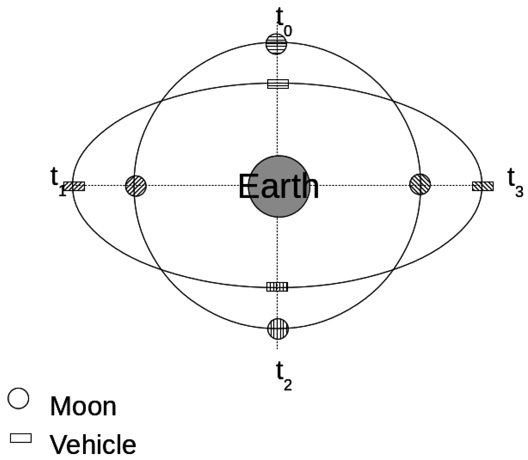
The 1:1:2 resonance looks somewhat similar to the 1:0:1 resonance, and is the most easily understood of the other resonances. In this pattern, the vehicle moves once around Moon as Moon moves once around the Earth–Moon barycenter. In a rotating frame, the trajectory is such that the vehicle appears to make 2 passes around Moon while completing that one orbit. Figure 2 illustrates snapshots of the trajectory for this resonance as observed in the Earth-centered inertial frame. Each snapshot of vehicle state is timestamped in sequence (t , t , t , t). As the vehicle passes through this sequence, the relative position changes are described as follows:
- The vehicle passes once around Earth in the inertial frame (above-left-below-right), moving counter-clockwise ().
- The moon passes once around Earth in the inertial frame (above-left-below-right), moving counter-clockwise ().
- The vehicle passes once around Moon in the inertial frame (below-left-above-right), moving clockwise (). Note that this is a retrograde motion.
- The vehicle passes twice around Moon in the rotating frame (near-side—far-side—near-side—far-side, where “near-side” means the vehicle is between Earth and Moon, and “far-side” means the moon is between the vehicle and Earth). This motion is also clockwise, or retrograde. ().
Notice that the vehicle orbit is quite definitely non-Keplerian. It is approximately elliptical, but with Earth at the center, not the focus, of the ellipse. This theoretical, geometrical solution is confirmed with simulation data. In Figure 3, the black line represents the lunar trajectory, and the red line the vehicular trajectory over a period of approximately 1 year. In this particular solution, the vehicular trajectory undergoes slow precession, the resonance is not perfect.
Of additional interest, this target DRO was used by Welch et al. [6] when investigating the potential cost-savings of using a powered lunar flyby as a strategy for injection into a DRO.
The 1:2:3 Resonance
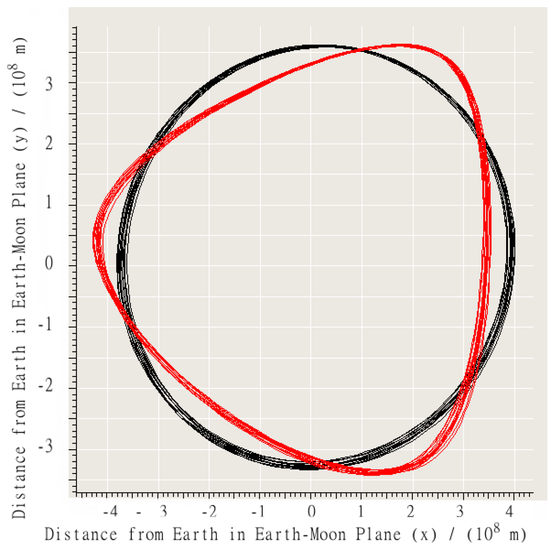
In one month, this resonance sees one prograde cycle of the vehicle relative to Earth, two retrograde cycles of the vehicle relative to Moon in the inertial frame, and three retrograde cycles of the vehicle relative to Moon in the rotating frame. Figure 4, again from simulation data, illustrates this pattern.
It is apparent now why we have retained the p term in the resonance identifier. The triangular trajectory in Figure 4 is more appropriately associated with the number 3 than with the number 2, even though it really is representing 2 inertial-cycles relative to Moon per inertial-cycle relative to Earth.
The 1:x:x+1 Resonances
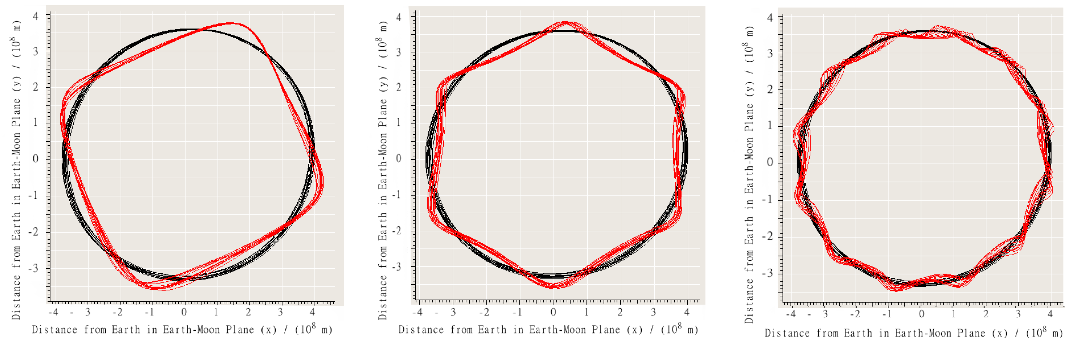
Higher order resonances are also easily found. A selection of these, the 1:3:4, 1:5:6, and 1:11:12 resonances, are shown in Figure 5.
The DRO period for one earth-centered position cycle is fixed at one month for these 1:x:x+1 patterns; thus as the order increases, the period for one moon-centered cycle must decrease accordingly. Consequently, the higher order resonances have smaller vehicle-moon distances. As the order increases and the vehicle-moon distance decreases, initially the DROs should become more stable. Bezrouk and Parker [7] demonstrated that solar gravity is the largest destabilizing influence for these resonances, so as the solar gravitational influence loses significance to lunar gravity, the stability should be enhanced. However, as the lunar gravity influence increases, the significance of its irregularities will also grow until they dominate as the major destabilizing factor. At the higher-order (and thus lower-altitude) resonances, such as 1:19:20 and higher, these lunar gravity irregularities will tend to make DROs less stable at lower altitude. Therefore, it is expected that there is a region of mid-altitude orbits that are stable, with stability degrading above and below these altitudes. This is confirmed in the simulation results, with the resonances becoming unstable at ratios greater than approximately 20. To find more DROs, it is necessary to keep the ratios low, thus requiring patterns on a multi-month timeframe, e.g., 2:3:5 = 2.5, and 3:4:7 = 2.33.
The 2:x:x+2 Resonances
Only those ratios comprising integers with no common denominator need to be considered, e.g., 2:1:3 and 2:3:5. The 2:2:4 resonance is identical to the 1:1:2 resonance.
No resonance was identified with a 2:1:3 ratio; the analysis presented in Section 2.2 confirms the complete absence of stable DROs at ratios below approximately 1.6. Additionally, while initial conditions were found for the 2:3:5 resonance, those conditions were not stable over a long period. Figure 6 represents the trajectory for a 2:3:5 resonance with data collected over approximately 1 year. The blue arrows identify the final pass before the stability collapses; it can be seen that the trajectory is starting to diverge from its cyclic pattern.
The 3:x:x+3 Resonances
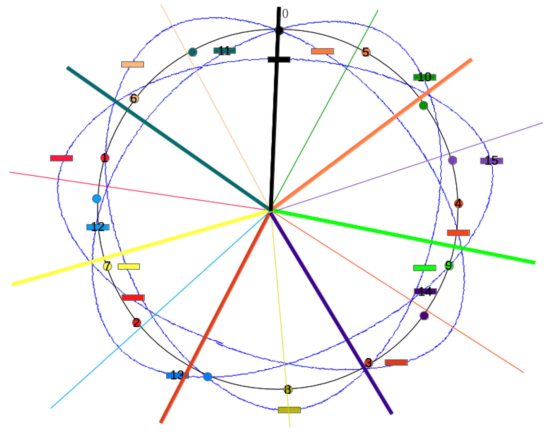
The 3:4:7 resonance was investigated and found to be stable over the long duration. With tri-monthly periods, the relative positions of the vehicle and Moon become difficult to visualize. Figure 7 shows the trajectory as in previous figures, and Figure 8 breaks that down into 16 steps, 4 steps per lunar orbit.
2.1.3. Longer Duration Resonances
Several long-duration stable ratios were identified, such as 6:5:11, 6:7:13, 7:8:15, 6:11:17, 3:8:11, etc. However, distinguishing and defining these higher orders becomes challenging. For example, a 4:5:9 resonance effectively completes 2.25 rotating-frame cycles per month, a value that neatly bridges the gap between 2 cycles of the 1:1:2 resonance and the 2.3 cycles of the 3:4:7 resonance. A state that is close to a perfect low-order resonance can easily be characterized as a slowly-precessing instance of that resonance. These states also tend to be stable.
Consequently, the distinction between a high-order long-duration resonance, such as 6:7:13, and a precessing low-order, short-duration resonance—such as 1:1:2—is small. The characterization of such a trajectory one way over another becomes completely arbitrary. Thus, nothing was considered with a period longer than 8-months.
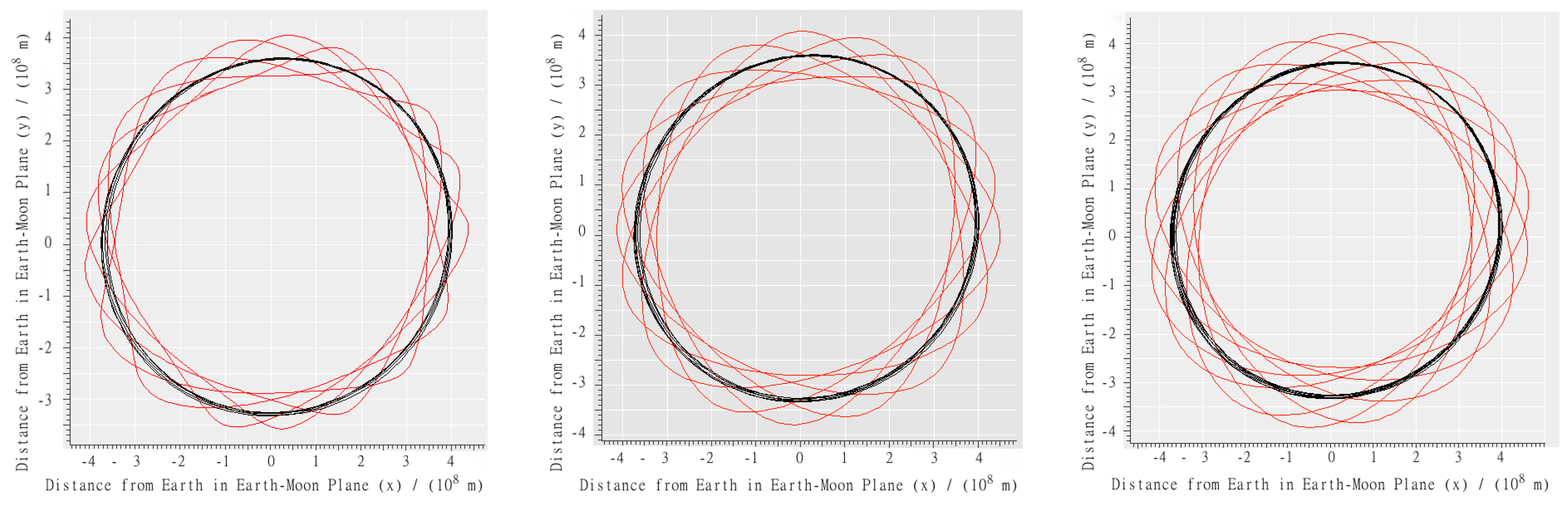
A selection of higher-order resonances is shown in Figure 9.
2.2. Analysis of the Stability of DROs
To categorize the state space, the vehicle state is initialized with two parameters:
- distance from Moon, along the Moon-to-Earth position vector, and
- Moon-relative velocity in the Earth–Moon orbital plane, perpendicular to the Moon–Earth position vector.
Note—the initial conditions are thus restricted to a plane coincident with the Earth–Moon orbital plane. It is anticipated that there will be additional stable conditions with velocities that include an initial out-of-plane component, but that lies beyond the scope of this study.
Equivalently, consider a frame rotating with the Earth–Moon system. Two such frames are widely used—the synodic frame, and the rectilinear local-vertical-local-horizontal (LVLH) reference frame (with origin at Moon, referenced to Earth). In the synodic frame, the initial vehicle state is characterized by
- the position, restricted to the range m (from Moon-center) along the negative x-axis, and
- the velocity, restricted to the range m·salong the positive y-axis.
In the LVLH frame, the initial vehicle state is characterized by
- the position, restricted to the range m along the positive z-axis, and
- the velocity, restricted to the range m·s along the positive x-axis.
We will continue with reference to the LVLH frame; for readers more familiar with the synodic frame, the transformation is:
- LVLH (complete the reference-frame) : Synodic
- LVLH (negative orbital angular momentum vector) : Synodic
- LVLH (Moon–Earth vector) : Synodic
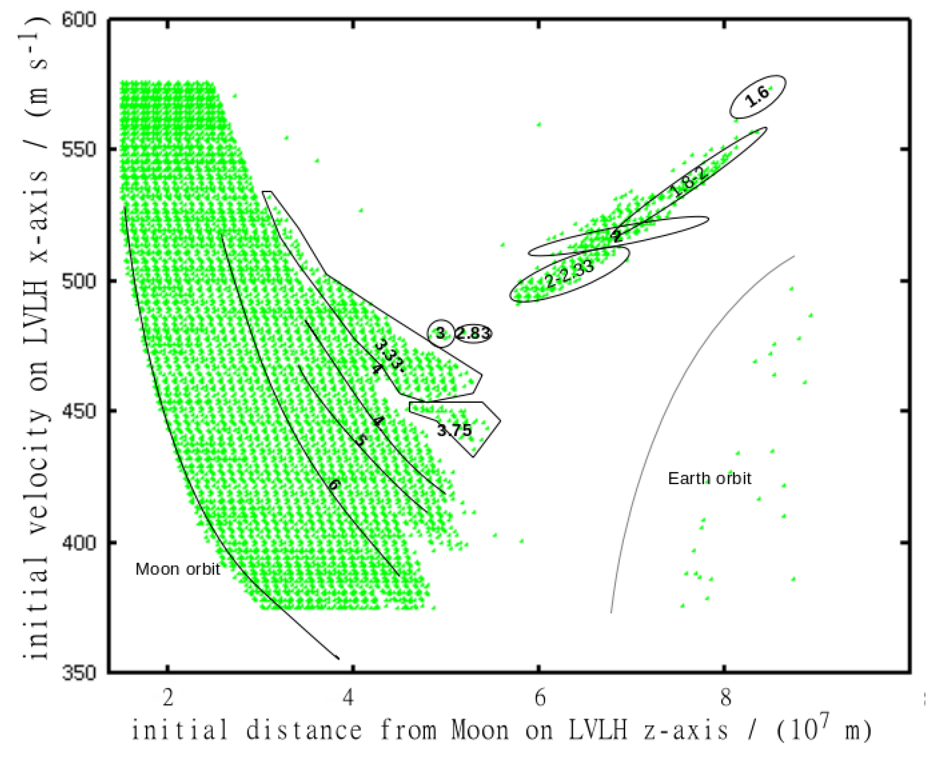
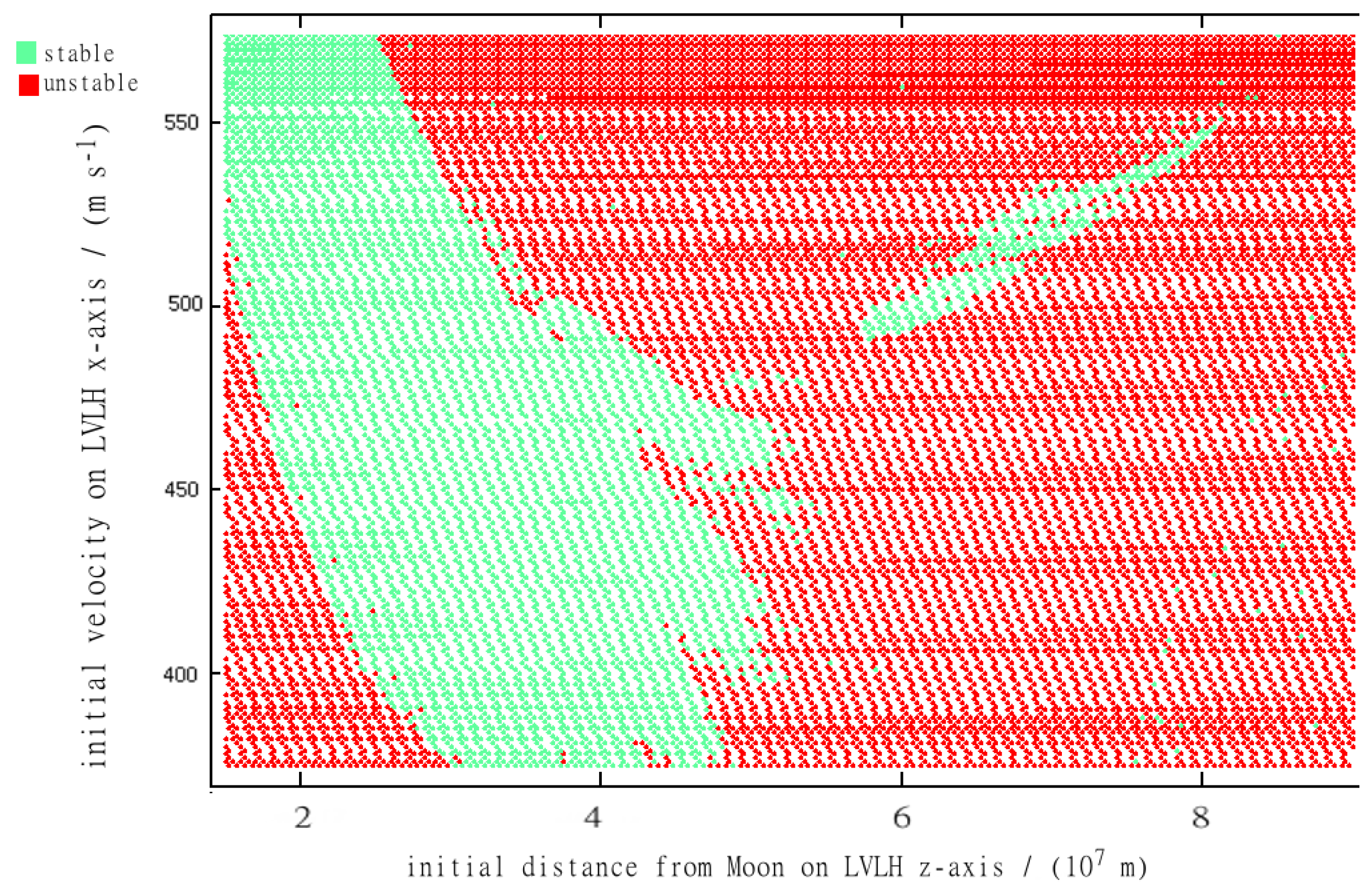
Figure 10 and Figure 11 illustrate which of these initial conditions produced trajectories that were stable for the 30-year duration of the simulation.
It should be noted that the small island of stable states between 60,000 km and 80,000 km is of most interest because of its energetically favorable location; this is also the region identified by Bezrouk and Parker [7] from their circular restricted three-body-problem analysis. Each resonant DRO has a range of initial conditions, resulting in a resonant-specific characteristic curve in this state-space. As the initial distance between vehicle and Moon is increased, the initial speed must decrease in order to maintain the resonance. Thus, at any given initial position, each specific resonance will have a specific initial velocity, with the higher ratios (e.g., 1:11:12) requiring a smaller speed than the lower ratios (e.g., 1:1:2).
Similarly, at any specific initial velocity, there are a number of possible initial positions available, with the lower ratio resonances found at higher lunar-altitudes. Thus, in Figure 10, the characteristic curves for higher ratio resonances will be found towards the lower-left, with those for lower ratios towards the upper-right.
Figure 11 shows a large region of stability at relatively low lunar-altitudes with isolated islands of stability at higher lunar-altitudes. The stable regions in state-space at higher latitude tend to be correlated with regions corresponding to resonances, but there are three very important observations here:
- Not all resonances are present;
- Of those that are present, the stable zones surrounding those characteristic curves are sized differently;
- the higher-order, lower-altitude resonances fall within a continuum of states that remain stable for the 30-year duration.
Those resonances with the larger stable zones will tend to be the more useful for stationing a vehicle for a long period of time. They are going to be easier to hit, and more stable against perturbing influences which may easily shift the state out of a small stable zone. See the discussion on radiation pressure (Section 2.4) for the significance of this consideration.
Analysis of Stable Zones
Notice from Figure 10 how the main region of stability covers ratios larger than 4. Between and 4 there are two separate regions, separated by a small region of instability. The 1:2:3 ratio is stable over only a very small range. A large gap—representing an absence of stable states—extends from ratio 3 (1:2:3) to (3:4:7), filled only by a couple of states in the 6:11:17 ratio which are of questionable stability. Of particular note, this means that there is no 2:3:5 () stable state.
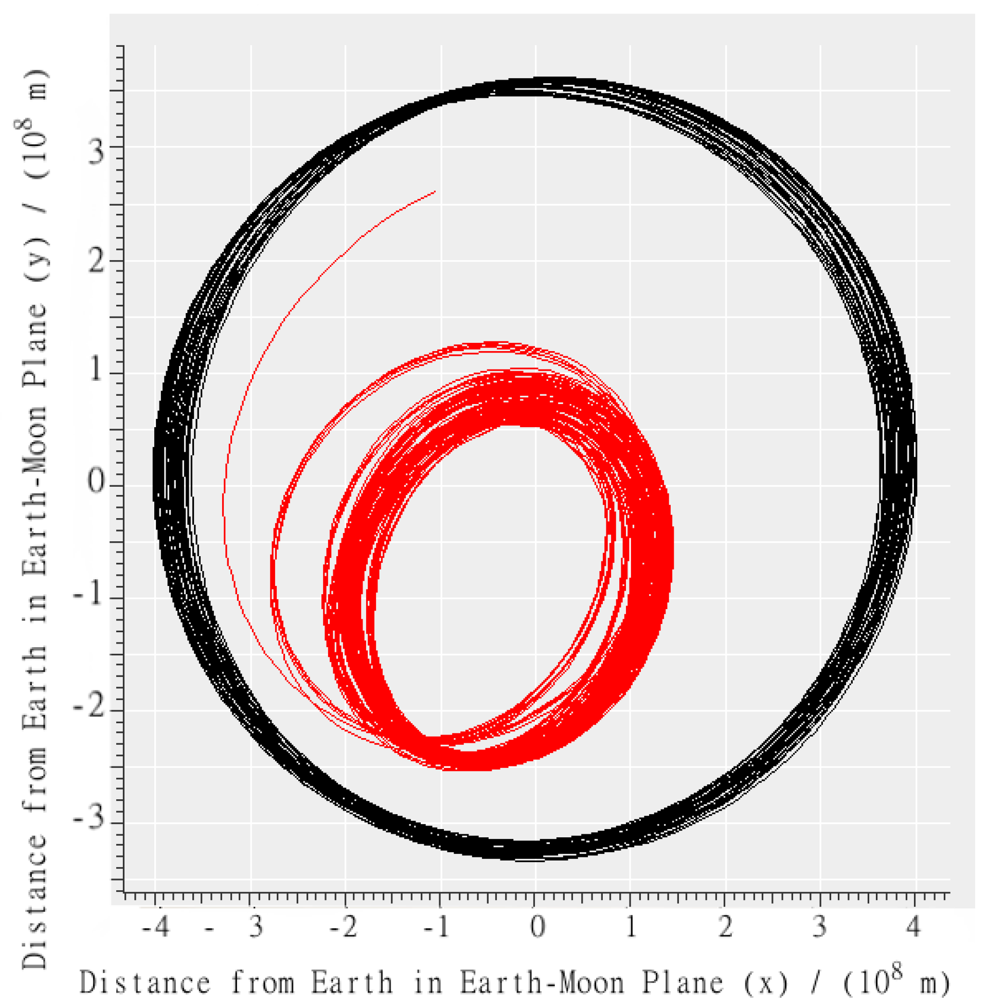
In the lower corners of Figure 10 and Figure 11, the vehicle goes into Moon and Earth orbits (left and right corners respectively). The orbits in the lower left corner are all unstable; there are some stable hits in the earth-orbit area, but these are not DROs; see Figure 12 for a characteristic trajectory from this region. These trajectories are unlikely to be stable in the long term and may well prove to be unstable in the simulated environment if the state were integrated differently. However, their presence here does raise the possibility of their potential use as “cycler-type” orbits requiring some limited degree of control authority to maintain stability.
Unstable trajectories are typically characterized as trajectories that have the vehicle coming close to Moon at some point and either crashing into it, or being ejected to a distance in excess of m. Such a trajectory could be a complete ejection from the Earth–Moon system, or result in a long-period return; in either case, the trajectory was rejected from consideration for stability.
In addition to the large islands of stable initial conditions, there are isolated initial states that generated stable states over the duration of the simulation; these may be associated with ‘sweet spots’ which result in eventual evolution onto a more stable orbit. Such orbital evolution is beyond the scope of this paper, but would be an interesting topic for further study.
The left-hand edge of the main stable zone is questionably stable. Here, the vehicle is heavily influenced by lunar gravity and pulled into an elliptical and rapidly varying trajectory around the moon. Typically, the period and periapsis can vary significantly from one pass to another, see Figure 13 for an example.
During the first few simulated months, closer examination of the trajectories associated with initial conditions along this edge (as in Figure 13) demonstrates significant irregularities. While there are a few isolated instances where the trajectory becomes sufficiently unstable to eject the vehicle from the study, most of our simulated vehicles that have initial conditions in this region eventually stabilize and remain in the simulation for the full 30 years. This long-term stability resulting from short-term instability again suggests a transition process from unstable to stable conditions. Additional examples are discussed later with some preliminary data, but this is an area that deserves significantly more study.
2.3. Long-Term Stability and Retention of Initial Conditions
2.3.1. Orbital Periods
Figure 13 illustrates a peculiar case in which the initial conditions produce a trajectory that appears to be quite unstable, but unexpectedly remains stable for the full 30-year simulation time. The presence of such conditions suggests that there may exist some mechanism to “attract” states from such a quasi-stable initial state-space into a more stable state-space. To further investigate this phenomenon, the evolution of stable trajectories is evaluated. The extent to which the state drifts away from the initial conditions is evaluated by testing for variations in the orbital periods of stable trajectories. For this study, the orbital period is defined as the time interval between subsequent crossings of the LVLH y–z plane, with position at positive-z (between Earth and Moon).
2.3.2. Variation in Orbital Periods
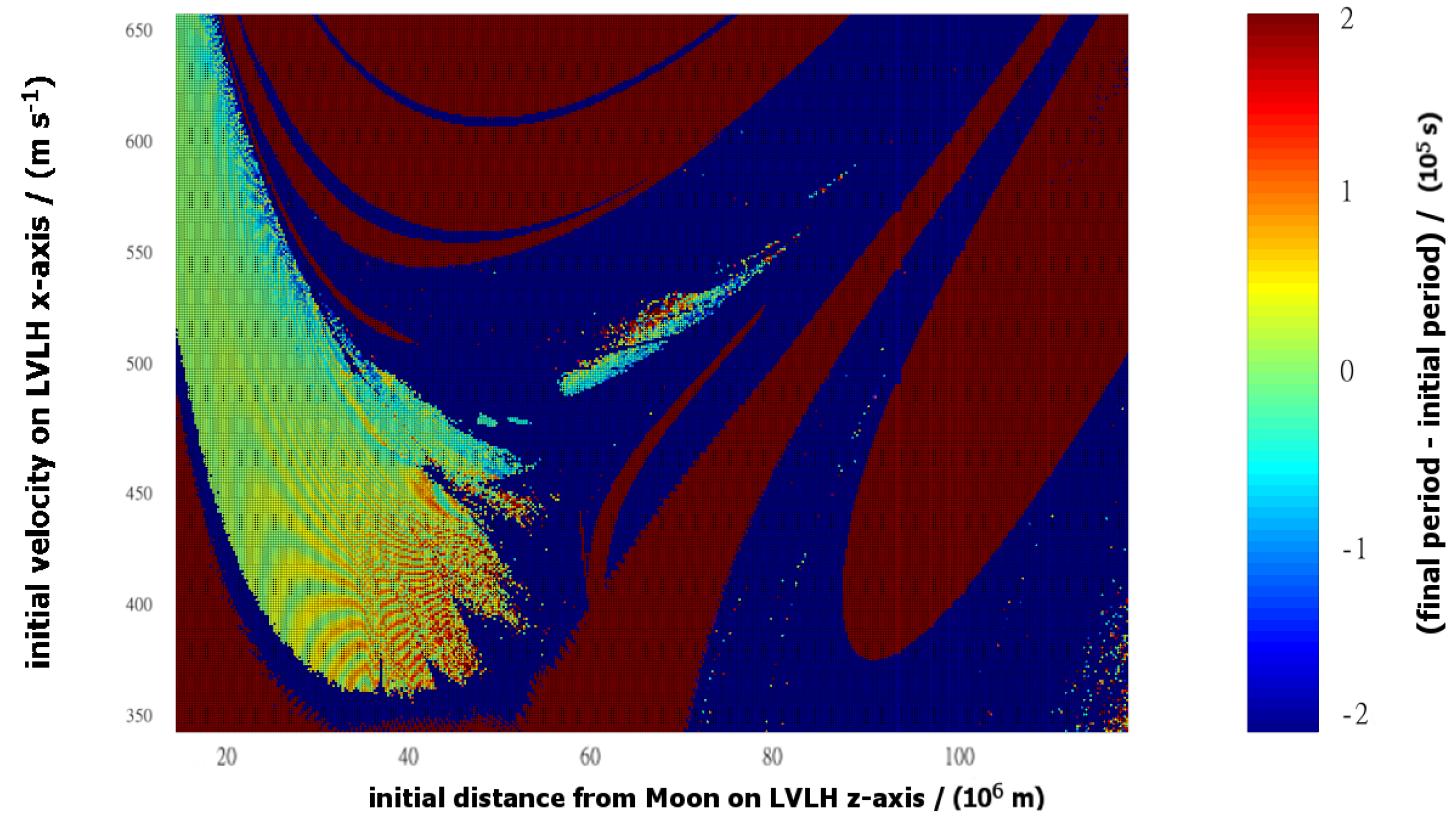
If the initial states identified in Figure 14 were asymptotically stable, then it would be expected that the initial periods and final periods (30 years later) would match. Conversely, a difference between initial and final periods for a vehicle that remains bound to Moon suggests an evolutionary process in the vehicle trajectory. In many cases, the comparison between the periods is close, but there are exceptions. The differences between the initial and final periods are shown in Figure 15.
There are some interesting features in Figure 15:
- In the stable island with m, the initial states on the lower right side tend to decrease in period, while the period of the states on the upper-left side tends to increase.
- The noticeable reduction in period along the upper right of the main island corresponds to region of that shows relatively high initial and final period (see Figure 14), and lies alongside a narrow strip of completely unstable initial conditions that failed to produce a single pass.
- The pattern of stripes seen at the low-velocity end of the main island are not at all understood. They could be artifacts of data selection, possibly a consequence of differencing only the single-values of initial period and final period in an area of state-space characterized by a continually evolving trajectory. This area requires additional study to be able to explain this feature.
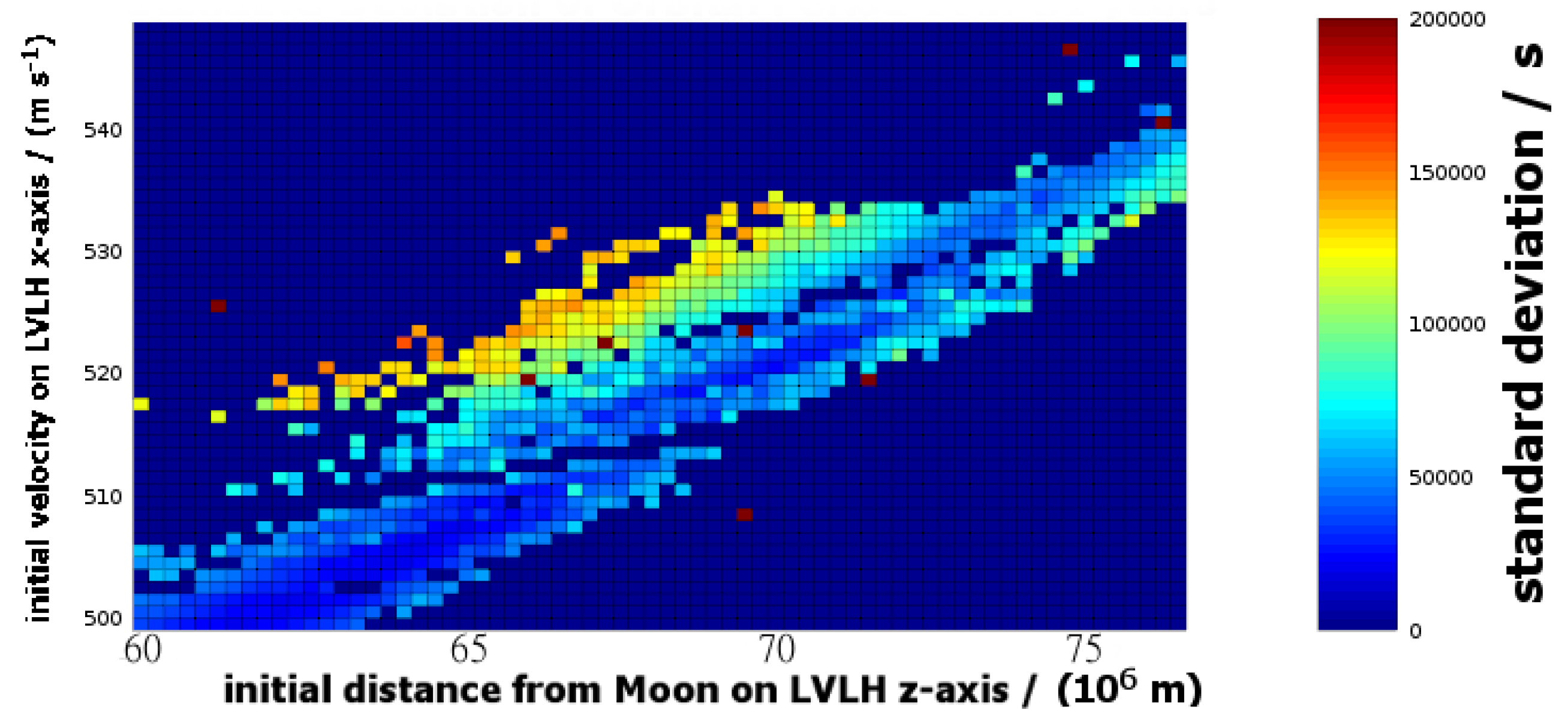
To further understand the stability of these orbits we need another single-valued characterization of the consistency of the periods throughout the entire thirty-year simulation. Conventional characterizations—such as trajectory plots and Poincaré sections are not applicable to large dispersed data sets because they inherently utilize two dimensions for presentation, and we only have one available. The alternative that can be useful is to consider the standard deviation of the period of each vehicle throughout its 30-year data-set. This is shown in Figure 16. Any initial states that lie close to asymptotically stable states would show consistent periods and consequently low standard deviation. Points of interest from Figure 16 are listed below and identified more clearly in the higher resolution images presented in Figure 17 and Figure 18. The causes of these features are not understood and warrant further investigation.
- the deep blue region in the center of the m island suggests that once established these orbits tend to be highly stable. Additionally, the initial conditions found in the upper-left area of this island show a significantly higher standard deviation than those states that lie in the lower-right area of this island. While it is expected that the initial conditions near the center line would be more stable, the asymmetry between the states “above” the center line and those “below” the line remains unexplained. This region is enhanced in Figure 17, and studied in more depth in Section 2.5.
- the features in the main island. These are illustrated further in Figure 18.
- A
- In the region m, m·s there are two regions of low standard deviation and a narrow line of high standard deviation separating them.
- B
- The lower left edge of the stable area described in A shows a sharp boundary (e.g., at m, 470 m·s). It appears almost as though there are two distinct dynamical processes, one in the background over a large range with a relatively large σ, and one with a smaller range and much lower σ that overrides the background process.
- C
- A line of locally high standard deviation cuts through the background from ( m, 550 m·s) to ( m, 450 m·s).
- D
- A line of relatively low standard deviation around ( m, 425 m·s) to ( m, 410 m·s). The finger of stability surrounding this line appears to be associated with a particular resonance (1:5:6). The low standard deviation on the line may be associated with the perfect resonance, and surrounded by states of near-resonance that are also stable.
2.4. Effect of Radiation Pressure
The effect of radiation pressure on the stability of a DRO is not possible to quantify in general terms because it depends on too many vehicle-specific parameters. The mass/volume ratio, the geometry of the surface, the rotational state, the albedo and emissivity, and the nature of the reflection all affect the extent to which solar radiation pressure can affect the vehicle trajectory. Furthermore, particularly in the regions where the stability is marginal, the Yarkovsky effect (differential thermal emissions) can be significant over such long durations. This will be affected by rotation rate; heat capacities and distribution of surface materials; thermal conductivity within the vehicle; and location of thermal sinks and sources, such as solar panels or other power generators, and radiators.
Nevertheless, it is worth considering the potential for solar radiation pressure to affect the stability of the trajectories studied thus far. The effect of including radiation pressure is not necessarily intuitive because there are competing factors. The effect of radiation pressure should counteract some of the solar gravitational perturbation, potentially leading to enhanced stability. However, particularly at low altitude where there will be significant periods of lunar shadowing, the radiation pressure will be selective in its application. It will be ineffective in shadow where lunar and solar gravity combine, and maximally effective where lunar and solar gravity are in opposition. It should also be noted that only direct solar radiation was considered; albedo effects from lunar and terrestrial reflection were not included. The results from simulation are that solar radiation pressure has a net de-stabilizing effect, particularly affecting those trajectories that were questionably stable (i.e., those states that lie along the edges of the green areas in Figure 11).
To test the effect, the vehicle was configured as a uniform isothermal sphere with perfect specular reflection. The simulations were terminated at five years (instead of thirty years) for reasons of simulation speed. There are some states that show stability in this case that were not stable before; it is not clear whether this is because radiation pressure stabilized them, or because they previously became unstable at some time between five and thirty years. However, the primary interest from this analysis is to identify whether there are trajectories that are de-stabilized by the presence of radiation pressure, not to identify isolated occurrences of potential stabilization. This is left to further work.
Three densities were tested:
- Very low density, kg·m. This test was intended to confirm whether radiation pressure perturbations could affect the stability of the trajectory.
- Low density, kg·m. This is still very low by spacecraft standards, but potentially relevant as a worst-case scenario for vehicles with large deployable arrays that would catch a significant pressure force without adding significantly to the mass. This effect is illustrated in Figure 19.
- Capsule-like density, kg·m. This is—to within an order of magnitude—comparable to a typical spacecraft capsule but still an order of magnitude below that of base materials. This effect is illustrated in Figure 20.
2.4.1. Very Low Density
Note—for reference, kg·m is a comparable density to that of a large empty mylar envelope, or vaguely equivalent to a mylar sheet; it should be expected that radiation pressure would provide an significant contribution to the net force. Indeed, at this level, the radiation force is comparable to the solar gravity which it opposes—and which the Earth-Moon barycenter continues to respond to—so it is expected that the vehicle will quickly leave the Earth–Moon system. The test was by no means exhaustive, but no stable trajectories were found.
2.4.2. Low Density
Figure 19 illustrates the overall effect of radiation pressure on the stability of a hypothetical low-density vehicle. The secondary islands of stability were effectively eliminated by this perturbation, leaving only the main region and a small region of stability around the 6:5:11 resonance. Of particular concern is the loss of almost all of the high-altitude stable region.
The plethora of isolated stable states seen in Figure 19 that was not seen in Figure 11 is mostly a consequence of the reduced simulation time. In isolated independent testing of some of these states, some remained to the end of the thirty-year period—just as there were isolated states that remained without radiation pressure—but most of the isolated test cases failed to reach thirty years.
2.4.3. Capsule-Like Density
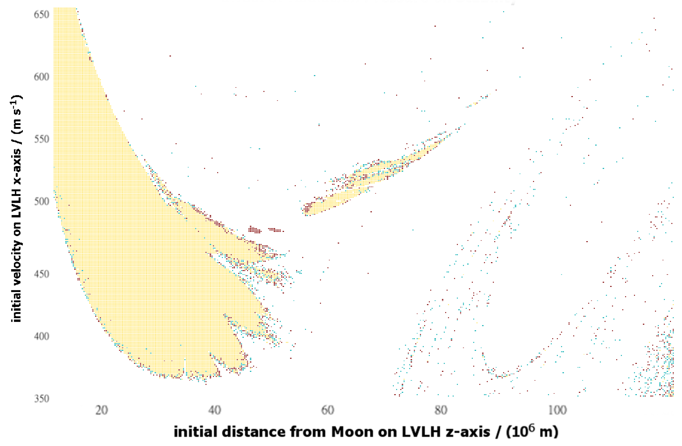
The results of the capsule-like density study are illustrated in Figure 20, using the full data set. With this density, radiation pressure had very little effect on the stability plots. The small “islands” previously seen in Figure 10 at 1:2:3 (ratio = 3) and at 6:11:17 (ratio = 2.83) are no longer stable, but the other regions are largely unaffected, with roughly equal numbers of the marginally-stable states around the edges transitioning each way between “stable” and “unstable”.
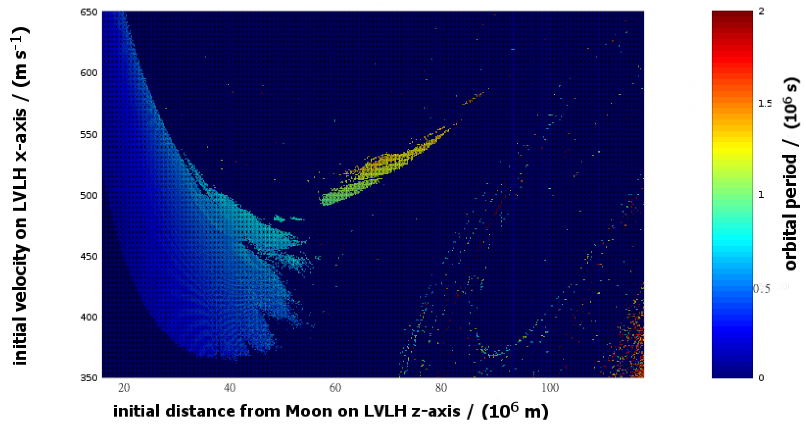
2.5. Detailed Study of the High-Altitude Stable Region
From Figure 20, five regions of stability were identified in the high-altitude, m, region; these are illustrated in Figure 21 and presented numerically in Table 1.
Characteristic data points are taken from the center of each region, thereby defining the region. The data including radiation pressure was used to identify the candidate profiles, but the data itself was then extracted from the longer 30-year run without radiation pressure.
Of these five, two are clearly associated with resonances, while three require the extension to higher orders, such as 7:6:13, or 7:8:15. Of interest is that the higher-order questionable resonances are symmetric about 2.0. Whether that is coincidental or a genuine feature of the dynamics is undetermined. But undeniably, the region with a period ratio of 2 is divided from the other stable conditions by instability bands; the reason why a period ratio of ( s) is stable when ( s) is not, and why ( s) is stable when ( s) is not understood and should be investigated further.
An additional effect appears when comparing the initial and final orbital period for each of the stable initial conditions. The variation with initial conditions of the initial orbital period is presented in Figure 22, while Figure 23 presents the variation with initial conditions of the final orbital period, some 30 years later. Both figures cover the same set of initial conditions, centered around the 1:1:2 resonance discussed in the previous paragraph. The dark blue regions represent those initial conditions that produce unstable trajectories.
Apparent from Figure 22, the initial period (color-axis) shows a strong dependency on the initial altitude (horizontal axis), as should be expected. However, it shows only a weak dependency on the initial velocity (vertical axis). The initial period varies continuously across the entire data set.
The values of the final period are very much more chaotic than the values for the initial period; this is somewhat expected given the high standard deviation for parts of this region (illustrated in Figure 17). Whereas the initial period showed a strong dependency on initial altitude, the final period appears to have more dependency on the initial velocity.
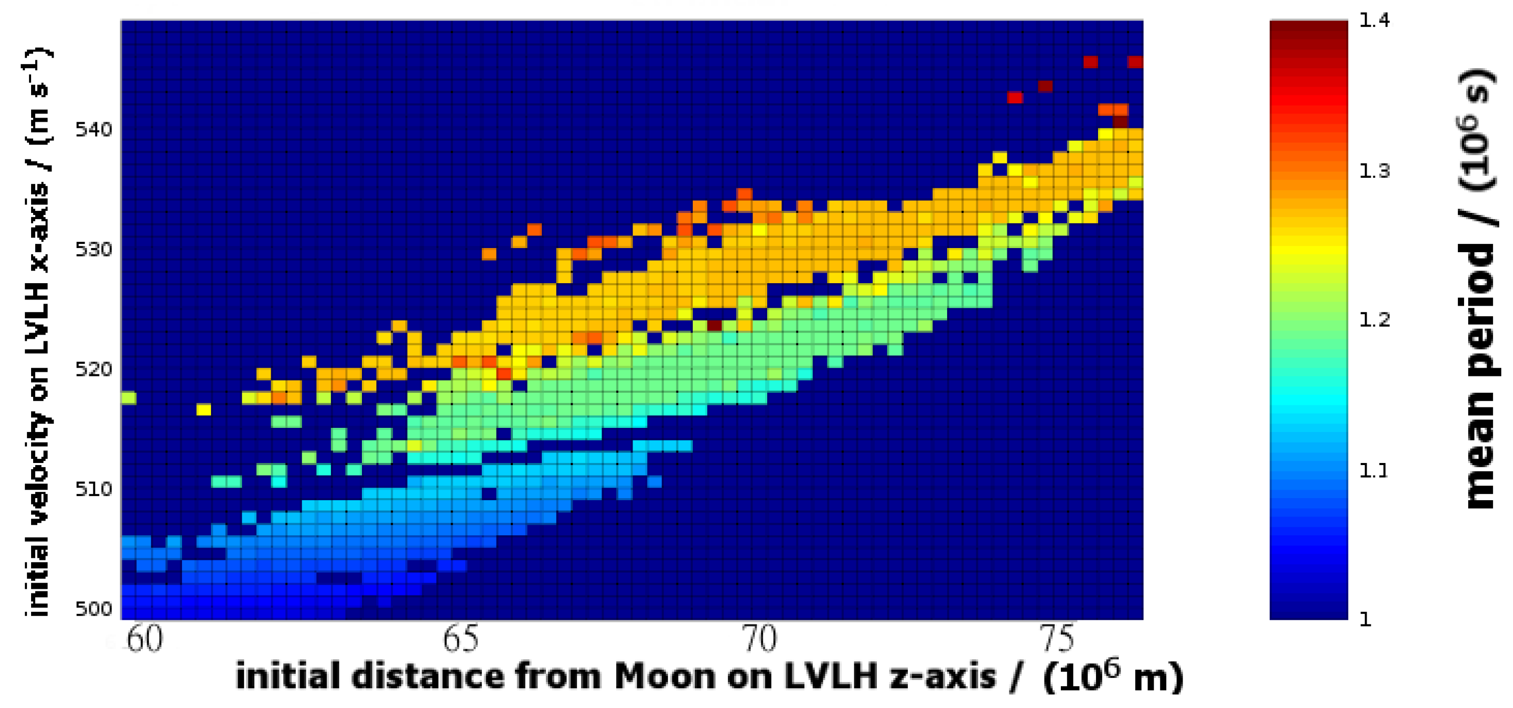
This change in dominant dependency is more noticeable when considering the mean orbital period, as shown in Figure 24. In addition to the dependency change, the mean period values are also very much more discrete than the initial period values. Initial states comprising the upper island (ratios of approximately 1.85) result in a near-uniform mean-period. Initial states comprising the center island (period ratios of approximately 2.0) result in another near-uniform mean-period, distinct from the upper island. Finally, initial states comprising the lower island (ratios of >2.0) result in a distribution of periods, but that distribution is still markedly different in nature than is the distribution of initial periods. The process by which the trajectories transition from those that produce the initial periods to those at the end of the run is not understood and needs further investigation.
3. Conclusions
In general, it is not safe to assume that an arbitrary lunar-retrograde trajectory in the Earth–Moon environment is stable. However, there are a range of DROs that show long-term stability (i.e., stable over the entire 30-year simulation) that may be suitable for parking and staging orbits. Potential injection/initial conditions for accessing those orbits between Earth and Moon have been explored and evaluated for stability. There are two distinct regions of position-velocity state-space that lead to trajectories that remain in the Earth–Moon system for 30 years—a “low altitude” region (below km from Moon) and a “high altitude” region (between km and km). The high-altitude region of stable DROs is characterized by a narrow range of acceptable velocities. Conversely, the low-altitude region provides a broad continuum of injection/initial conditions that lead to relatively stable trajectories.
3.1. Significance of Resonances
Some ratios have obviously resonant associations. For example, the integers and half-integers (e.g., , or 2:3:5, conceptually completes five lunar orbits every two months) are clear. Less obvious are the more exotic values (e.g., completes 11 lunar cycles in 6 months—i.e., 6:5:11). The analysis of whether resonance enhances stability is inconclusive. It is certainly not a determining factor; there are some very basic resonances (e.g., ) that have no identifiable initial/injection conditions, and many that are stable only over a narrow region of state-space (e.g., ). In the high-altitude stable region, there appears to be a correlation between the regions of position-velocity state-space that produce stable DROs and those that produce resonant DROs. However, in the lower altitude region, there is a broad continuum of stable initial-conditions, and resonance appears to be of little significance.
Even in the high-altitude region, there exist stable initial-conditions that do not produce a perfect resonance, such as with a ratio. This could arguably be interpreted as a forward-precessing 1:1:2 resonant state (2-and-a-bit cycles per month), or an independent, non-resonant, state. The choice is entirely arbitrary. However, these off-resonant trajectories tend to exhibit more evolution in their trajectories than the resonant states (e.g., 2.33, 3:4:7) in the same region. The resonant states tend to exhibit lower standard deviation in their orbital period over the full 30-year simulation, and have been demonstrated to follow a consistent path over several months, suggesting possible asymptotic stability. An interesting area for further study might be a comparison of the evolution of a perfect-resonant trajectory with a slightly off-resonant trajectory with slightly different initial/injection conditions.
3.2. Addition of Perturbations
The addition of radiation pressure as another perturbing force has been demonstrated to further degrade the stability of the DROs, but minimally so at capsule-like densities and higher. This result implies that vehicle configuration should be an important consideration in determining the long-term stability of parking a vehicle in a DRO. Particular attention is required with the presence of relatively large surfaces—such as solar panels—that tend to increase the significance of radiation pressure realtive to gravity effects.
3.3. Access to DROs
The results from this paper illustrate a range of initial or injection states that can results in stable DRO trajectories, with a broad range of injection positions and velocities available. The study is limited to injection states that are initially in-plane and accessed at a location between Earth and Moon. A similar study would be useful for injection states for accessing DROs on the lunar far-side.
The injection velocities presented throughout this paper are relative to the rotating Earth–Moon vector. With injection-positions being between Earth and Moon, the corresponding injection-velocities in the inertial-frame are the sum of the values presented herein and the velocity of the respective injection-position through inertial-space. The resulting net injection-velocity for direct injection from a simple transfer from Low Earth Orbit is in the vicinity of 1 km·s. Consequently, it does not appear that there are any near-side direct-injections into stable DRO trajectories that would be within the capabilities of small satellite projects.
Acknowledgments
I would like to acknowledge Robert Shelton for recognizing the potential significance of this work, encouraging its publication, and for reviewing the document.
Conflicts of Interest
The author declares no conflict of interest.
References
- O’Campo, C.A.; Rosborough, G.W. Transfer Trajectories for Distant Retrograde Orbiters of the Earth; Recon Technical Report A 95:81418 1993; NASA STI: Hampton, VA, USA, 1993; 0065-3438pp. 1177–1200.
- Hénon, M. Numerical exploration of the restricted problem. VI. Hill’s case: Non-periodic orbits. Astron. Astrophys. 1970, 9, 24–36. [Google Scholar]
- Conte, D.; Di Carlo, M.; Ho, K.; Spencer, D.B.; Vasile, M. Earth-Mars Transfers through Moon Distant Retrograde Orbit. In Proceedings of the AAS/AIAA Astrodynamics Specialist Conference, Vail, CO, USA, 9–13 August 2015.
- Ming, X.; Shijie, X. Exploration of distant retrograde orbits around Moon. Acta Astronaut. 2007, 65, 853–860. [Google Scholar] [CrossRef]
- Tan, M.; Zhang, K.; Lv, M.; Xing, C. Transfer to long term distant retrograde orbits around the Moon. Acta Astronaut. 2014, 98, 50–63. [Google Scholar]
- Welch, C.M.; Parker, J.S.; Buxton, C. Mission Considerations for Transfers to a Distant Retrograde Orbit. J. Astronaut. Sci. 2015, 62, 101–124. [Google Scholar] [CrossRef]
- Bezrouk, C.; Parker, J. Long Duration Stability of Distant Retrograde Orbits. In Proceedings of the AIAA/AAS Astrodynamics Specialist Conference, San Diego, CA, USA, 4–7 August 2014.
- Jackson, A.A.; Thebeau, C.D. JSC Engineering Orbital Dynamics Top Level Document; NASA Technical Report JSC-61777-docs; National Aeronautics and Space Administration: Houston, TX, USA, 2012.
- Radhakrishnan, K.; Hindmarsh, A.C. Description and Use of LSODE, the Livermore Solver for Ordinary Differential Equations; NASA Reference Publ. 1327; National Aeronautics and Space Administration: Houston, TX, USA, 1993.
- Hammen, D.; Turner, G. JSC Engineering Orbital Dynamics Integration Model; NASA Technical Report JSC-61777-utils/integration; National Aeronautics and Space Administration: Houston, TX, USA, 2012.
- Berry, M.M.; Healy, L.M. Implementation of Gauss-Jackson integration for orbit propagation. J. Astronaut. Sci. 2004, 52, 331–357. [Google Scholar]
- Spencer, A.; Morris, J. JSC Engineering Orbital Dynamics Rotation, Nutation, and Precession Model; NASA Technical Report JSC-61777-environment/RNP; National Aeronautics and Space Administration: Houston, TX, USA, 2012.
- Bond, V.R. The RNP Routine for the Standard Epoch J2000; NASA Technical Report NASA:JSC-24574; National Aeronautics and Space Administration: Houston, TX, USA, 1990.
- Murray, C.D.; Dermott, S.F. Solar System Dynamics; Cambridge University Press: Cambridge, UK, 1999; ISBN 0-521-57297-4. [Google Scholar]
Figure 1.
Schematic of the conceptual 1:0:1 resonance. The solid lines represent the path through the inertial frame for two different orbits. The dashed lines indicate the relative position of the two vehicles at snapshots in time.
Figure 1.
Schematic of the conceptual 1:0:1 resonance. The solid lines represent the path through the inertial frame for two different orbits. The dashed lines indicate the relative position of the two vehicles at snapshots in time.
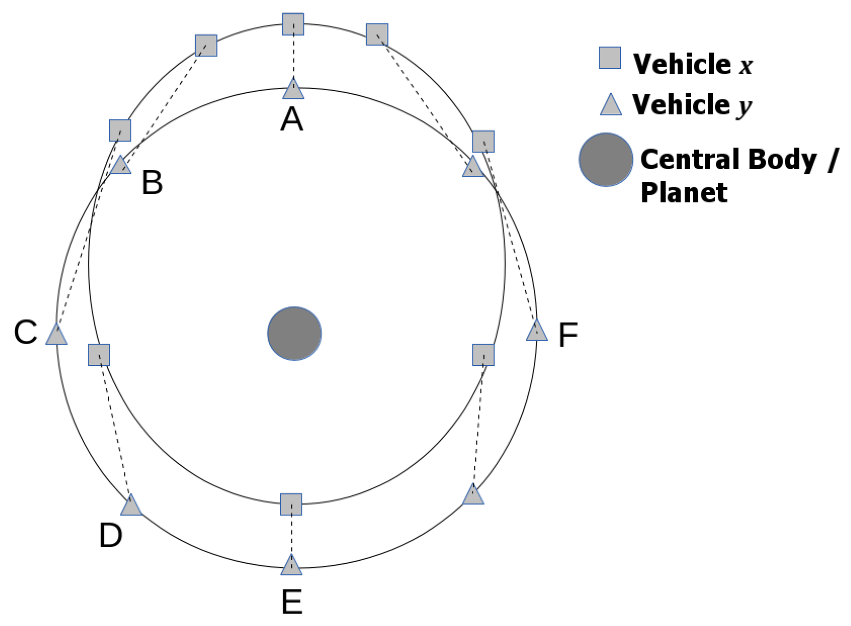
Figure 2.
Illustration of the 1:1:2 resonance. The illustrated trajectories are shown in the Earth-centered inertial frame.
Figure 2.
Illustration of the 1:1:2 resonance. The illustrated trajectories are shown in the Earth-centered inertial frame.

Figure 3.
A slowly precessing 1:1:2 resonance. The black line (circular trajectory) represents the lunar orbit relative to the Earth-centered inertial-frame, and the red line (precessing oval trajectory) the Distant Retrograde Orbit (DRO) trajectory relative to the Earth-centered inertial frame. Earth is at plot-center.
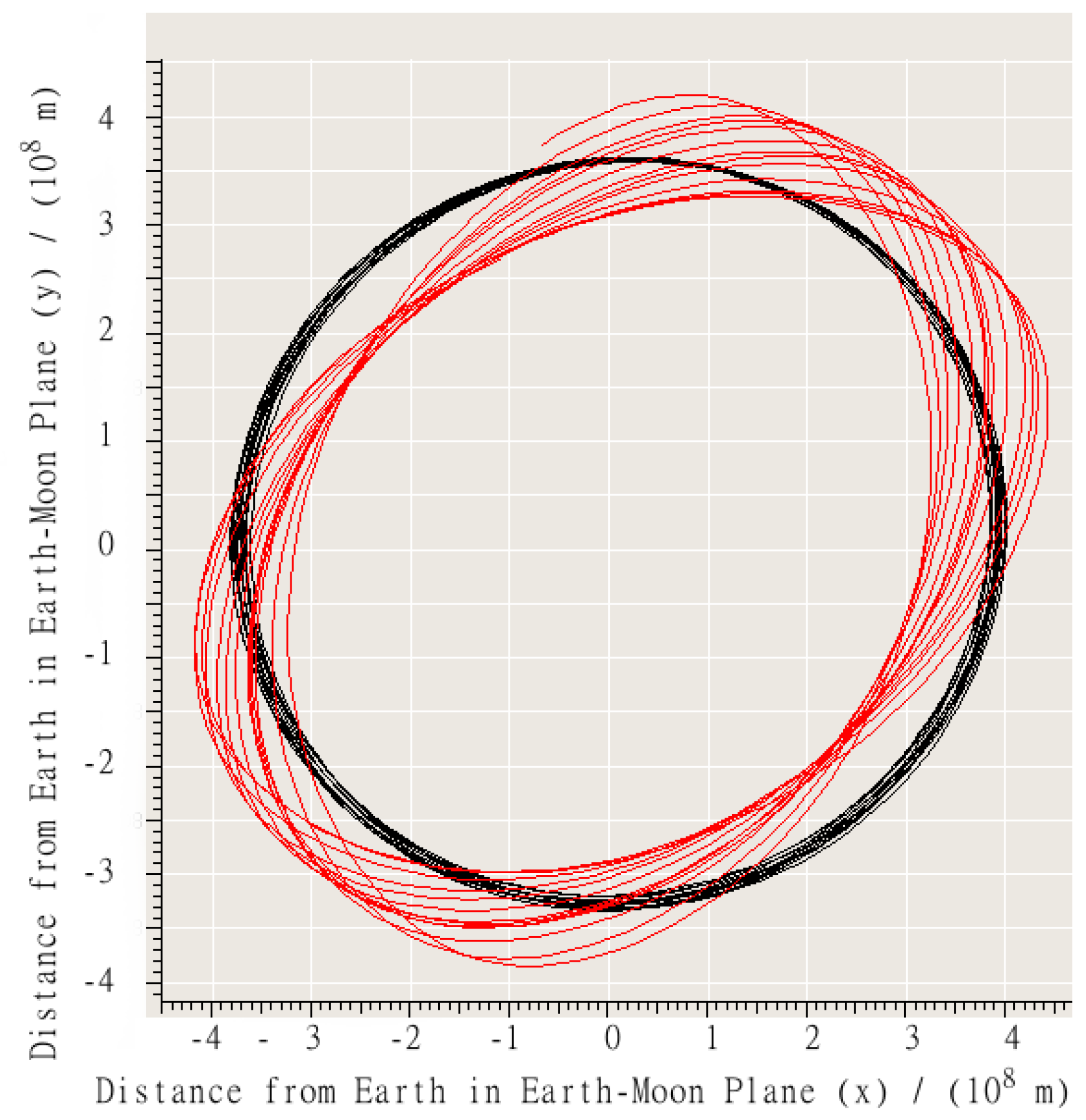
Figure 4.
The 1:2:3 Resonance. The black line (circular trajectory) represents the lunar orbit relative to the Earth-centered inertial-frame, and the red line (precessing oval trajectory) the DRO trajectory relative to the Earth-centered inertial frame. Earth is at plot-center.
Figure 4.
The 1:2:3 Resonance. The black line (circular trajectory) represents the lunar orbit relative to the Earth-centered inertial-frame, and the red line (precessing oval trajectory) the DRO trajectory relative to the Earth-centered inertial frame. Earth is at plot-center.

Figure 5.
The 1:3:4 (left), 1:5:6 (center), and 1:11:12 (right) Resonances. In each plot, the black line (circular trajectory) represents the lunar orbit, and the red line (non-circular trajectory) the DRO. Both trajectories are shown relative to the inertial frame; the lines illustrate the respective trajectory on the Earth–Moon plane in the Earth-centered inertial frame.

Figure 6.
The 2:3:5 Resonance. The black line (circular trajectory) represents the lunar orbit, and the red line (irregular trajectory) the DRO. This trajectory was stable for only approximately 1 year; the final pass is identified with the blue arrows showing the divergence of the trajectory from its initially-settled path. The vehicle had a close lunar encounter and was ejected from the Earth–Moon system shortly after this data set was captured.
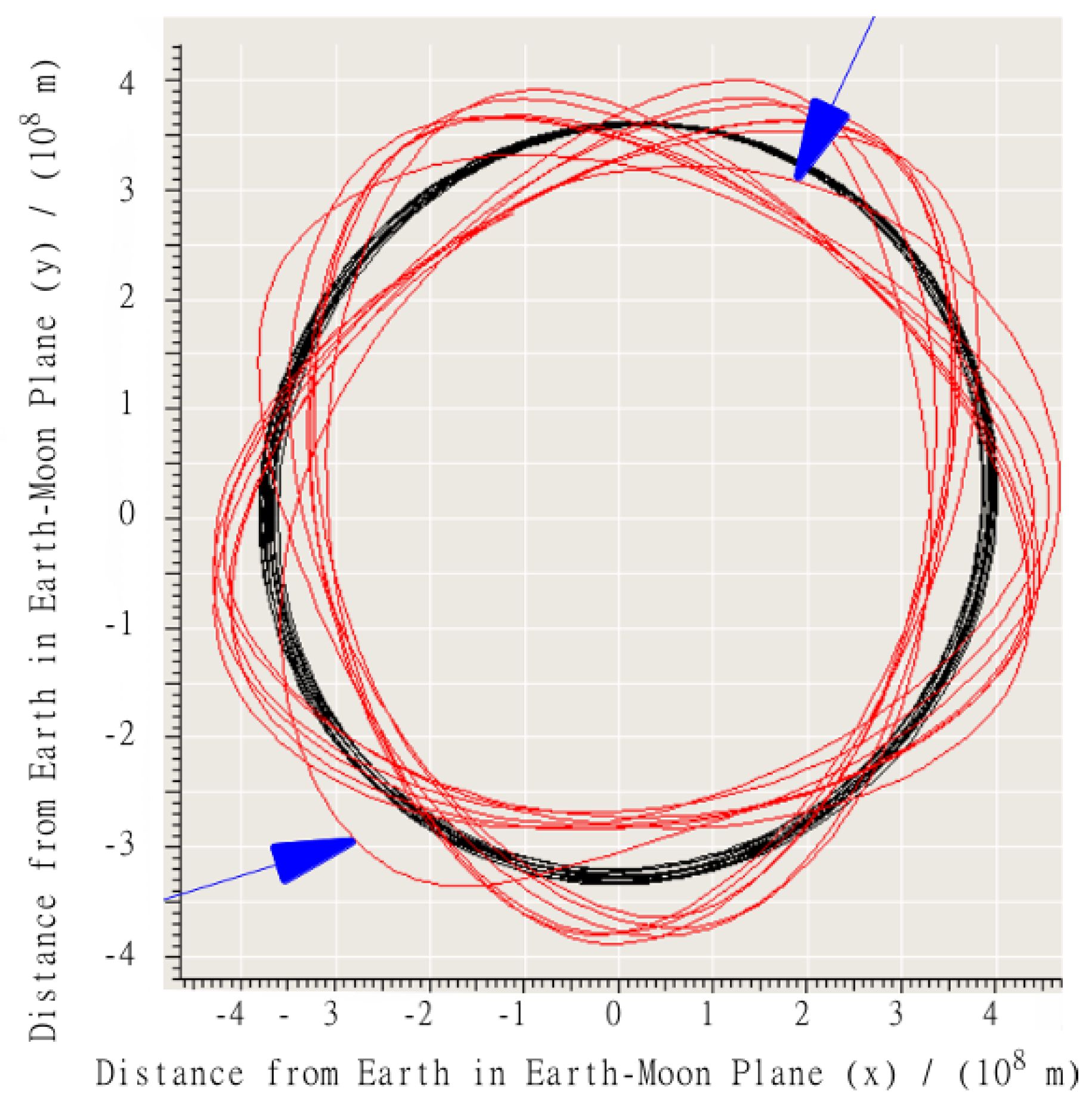
Figure 7.
The 3:4:7 Resonance. The black line (circular trajectory) represents the lunar orbit, and the red line (7-pointed star) the DRO.
Figure 7.
The 3:4:7 Resonance. The black line (circular trajectory) represents the lunar orbit, and the red line (7-pointed star) the DRO.
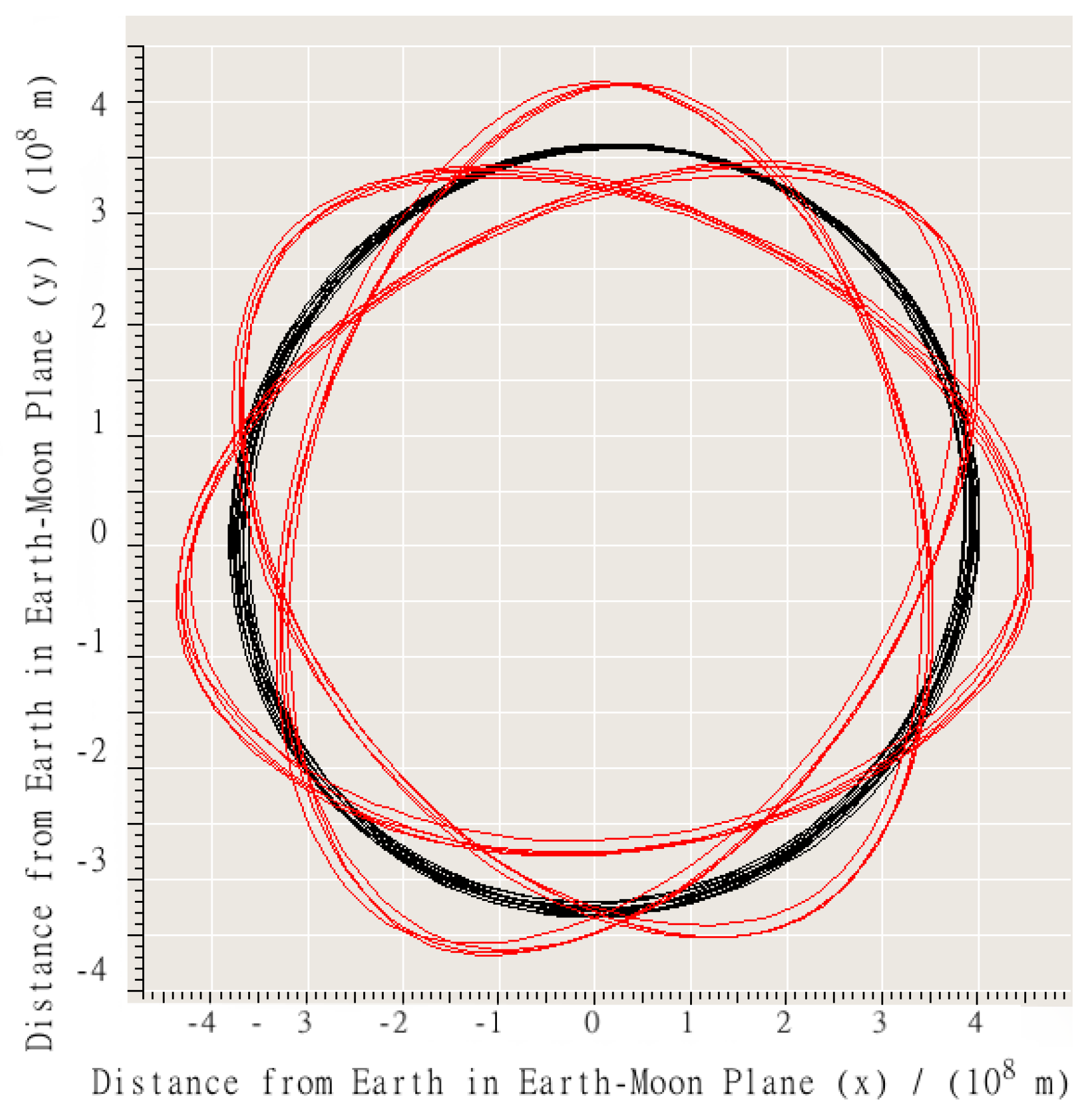
Figure 8.
A timestamp breakdown of the 3:4:7 resonance in the Earth-centered inertial frame. Each timestamp includes a moon (small solid circle) and vehicle (rectangle). The moon and vehicle are color-matched, and each timestamp sequentially numbered. The grey circular line (on which the small circles are found) represents the trajectory of the moon, and the blue irregular line represents the trajectory of the vehicle. Starting at the top (black,0), both the moon and vehicle trace three earth-orbits before returning to the black state. The color-coordinated numerical sequence illustrates each quarter of the four lunar-orbits. The radial lines approximate the positions at which the vehicle is at inferior (thick lines) and superior (thin lines) locations relative to the moon; together, they illustrate the seven cycles in the rotating frame. The radial lines are color-coded to be close to the colors at a nearby time-stamp.

Figure 9.
The 5:14:19 (3.8) (left); 6:11:17 (2.83) (center); and 8:9:17 (2.12) (right) resonances. In each plot, the black line (circular trajectory) represents the lunar orbit, and the red line (complex pattern) the DRO. Notice the peak altitudes increase as the ratio decreases.
Figure 9.
The 5:14:19 (3.8) (left); 6:11:17 (2.83) (center); and 8:9:17 (2.12) (right) resonances. In each plot, the black line (circular trajectory) represents the lunar orbit, and the red line (complex pattern) the DRO. Notice the peak altitudes increase as the ratio decreases.

Figure 10.
The initial states (shown in green) that remain stable over 30 years. The horizontal axis represents the initial position, measured along the local-vertical-local-horizontal (LVLH) z-axis; the vertical axis represents the initial velocity, directed along the LVLH x-axis. In the lower left, the states are sufficiently slow and close to the moon that they enter a lunar orbit. In the lower right, the vehicle never reaches Lunar orbit and instead enters an Earth quasi-periodic orbit. The numbers in the various regions indicate the approximate resonance ratios (e.g., 1:1:2 = 2; 4:11:15 = 3.75), as determined by investigation of orbital characteristics in these regions.

Figure 11.
Superposition of the stable states from Figure 10 and the corresponding unstable initial states. Green (light shading) represents stable states, red (dark shading) represents unstable states. See also Figures 14 or 20 for more comprehensive data sets.
Figure 11.
Superposition of the stable states from Figure 10 and the corresponding unstable initial states. Green (light shading) represents stable states, red (dark shading) represents unstable states. See also Figures 14 or 20 for more comprehensive data sets.

Figure 12.
A characteristic trajectory in earth-inertial for a state taken from the lower right corner of the stability plot. The axes represent positions in the earth-centered reference frame. The black line (outer loop, circular trajectory) represents the moon’s trajectory. The red line (inner loop) represents the vehicle trajectory. This is not representative of a DRO and its stability is highly questionable. There is potential for this type of orbit to be useful with the availability of some control authority.

Figure 13.
A characteristic trajectory over 1 month from the left-edge of the main stable zone in earth-centered coordinates. The black line (smooth circular shape) represents the trajectory of Moon. The red line (irregular pattern) represents the trajectory of a vehicle that was ultimately stable for 30 years.

Figure 14.
The final period between crossings of the LVLH y–z plane for those initial conditions that produced 30-year-stable trajectories. The time interval is shown in seconds on the color-axis as a function of the initial state. The horizontal axis represents the initial poisiton (meters), measured along the LVLH z-axis; the vertical axis represents the initial velocity (m/s), directed parallel to the LVLH x-axis. For reference, 1 sidereal month is approximately s. This plot can also be used to identify the 30-year-stable initial conditions. As such, it is similar to Figure 11, but provides more detailed coverage of the initial states.

Figure 15.
The difference in orbital periods between the period between the first positive-directed intersections with the y–z plane, and the period between the last recorded intersections of the same. The initial conditions that are not stable over 30 years are also shown. Those initial conditions that fail to produce a pass through the y–z plane are shaded dark red; those that complete one pass and subsequently become unstable are shaded dark blue.

Figure 16.
The standard deviation of the orbital period (color-axis) as a function of the initial state. As with Figure 15, the horizontal axis represents initial position (m) on the z-axis of the LVLH frame and the vertical axis represents the initial velocity (m·s) along the x-axis of the LVLH frame.
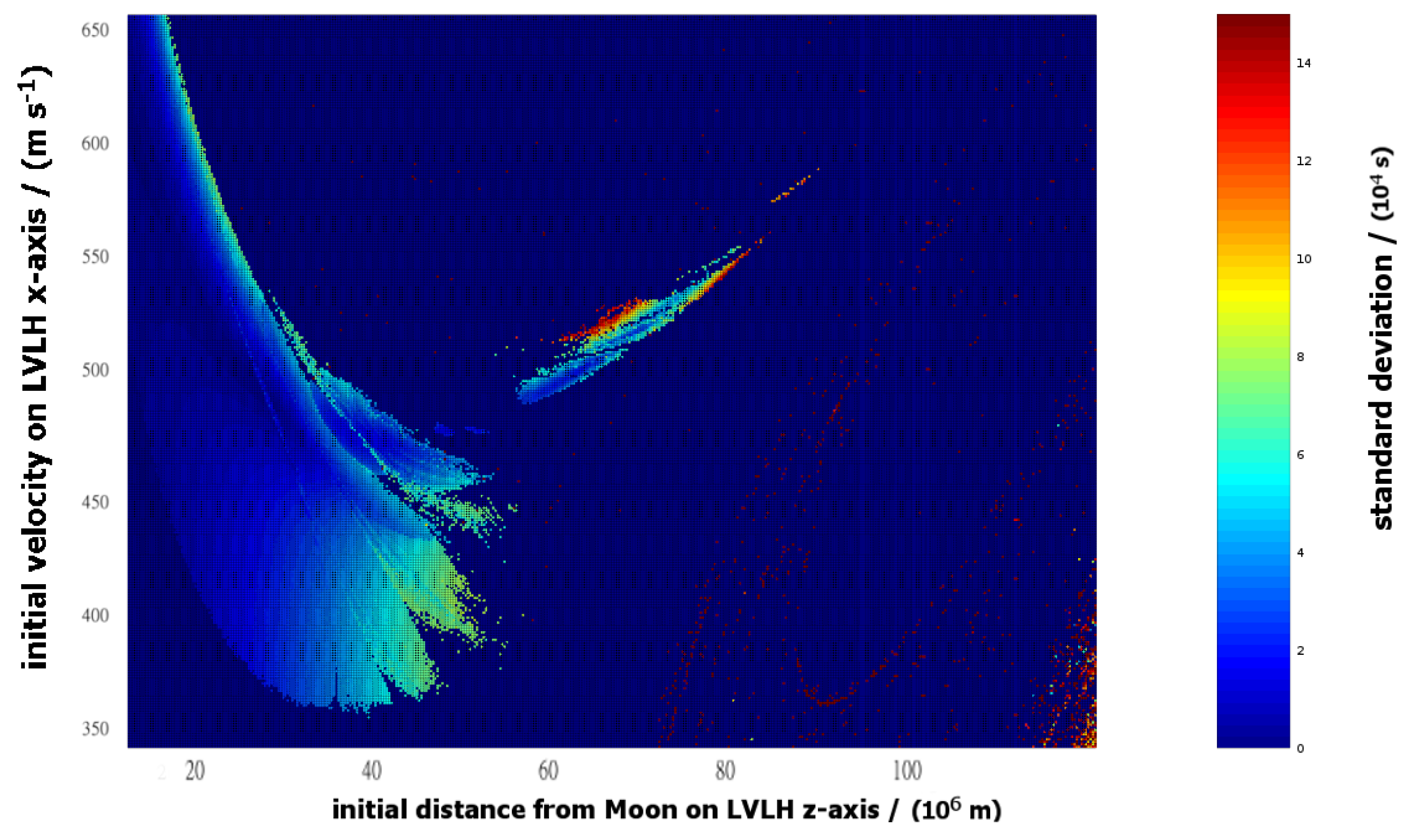
Figure 17.
Replica of Figure 16 with higher resolution on the high-altitude region of interest.
Figure 17.
Replica of Figure 16 with higher resolution on the high-altitude region of interest.

Figure 18.
Replica of Figure 16 identifying regions of interest (A–D) as discussed in this section.
Figure 18.
Replica of Figure 16 identifying regions of interest (A–D) as discussed in this section.
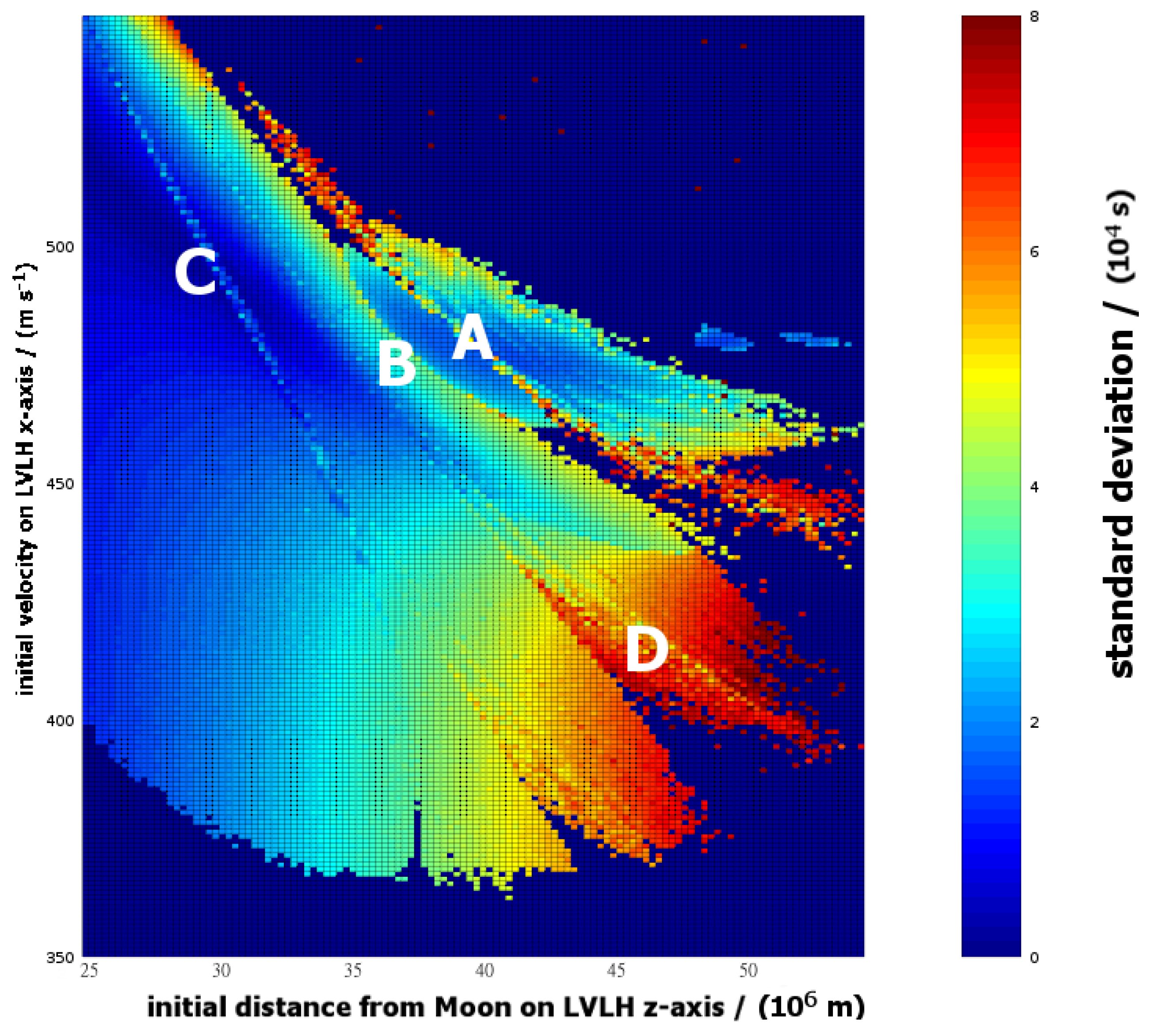
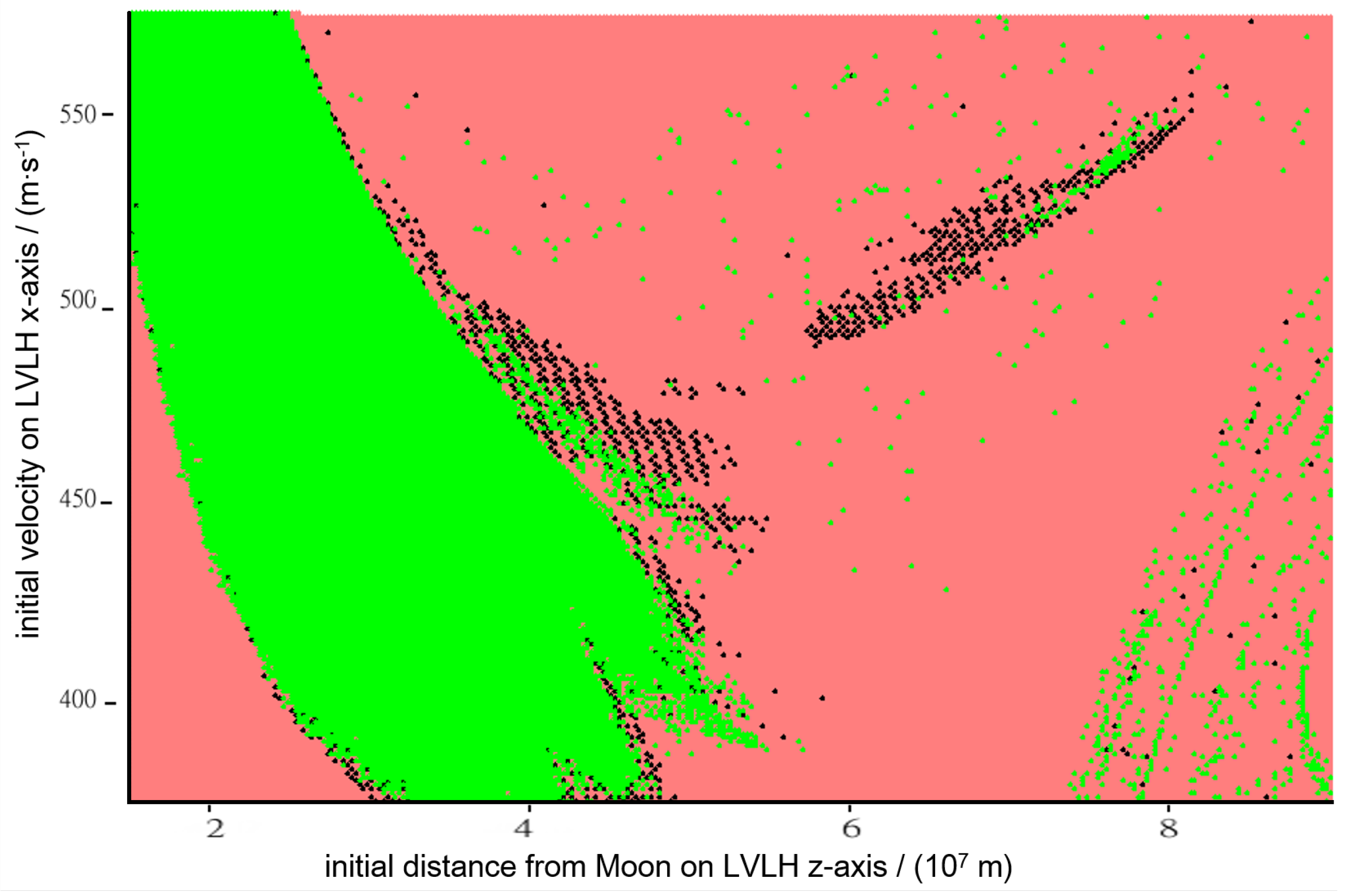
Figure 19.
Superposition of the stable (green/light shading) and unstable (red/darker shading) states for the case with radiation pressure. States that were stable without radiation pressure and unstable with radiation pressure are identified with black dots. Most of the minor zones of stability have been destabilized by the effect of radiation pressure. Note—the black dots are taken from the limited data set used to generate Figure 10 and Figure 11 and are set against a higher resolution data set. Consider the black dots as representative of area-shading rather than specific states.

Figure 20.
Graphical representation of the effect of radiation pressure on the stability of DROs. The horizontal axis represents the initial position (m), measured along the LVLH z-axis; the vertical axis represents the initial velocity (m·s), directed along the LVLH x-axis. The color axis is interpreted as: Yellow/light shading—initial conditions that produce 30-year-stable trajectories without radiation pressure and 5-year-stable trajectories with radiation pressure; Blue/medium shading—initial conditions that produce 5-year-stable trajectories with radiation pressure but did not produce 30-year-stable trajectories in the non-radiation pressure data set; Red/dark shading—initial conditions that produce 30-year-stable trajectories without radiation pressure but fail to do so with radiation pressure.

Figure 21.
Identification of the five points (A–E) representing the centers of the stable islands in the high-altitude stable area. These data points are presented numerically in Table 1.
Figure 21.
Identification of the five points (A–E) representing the centers of the stable islands in the high-altitude stable area. These data points are presented numerically in Table 1.
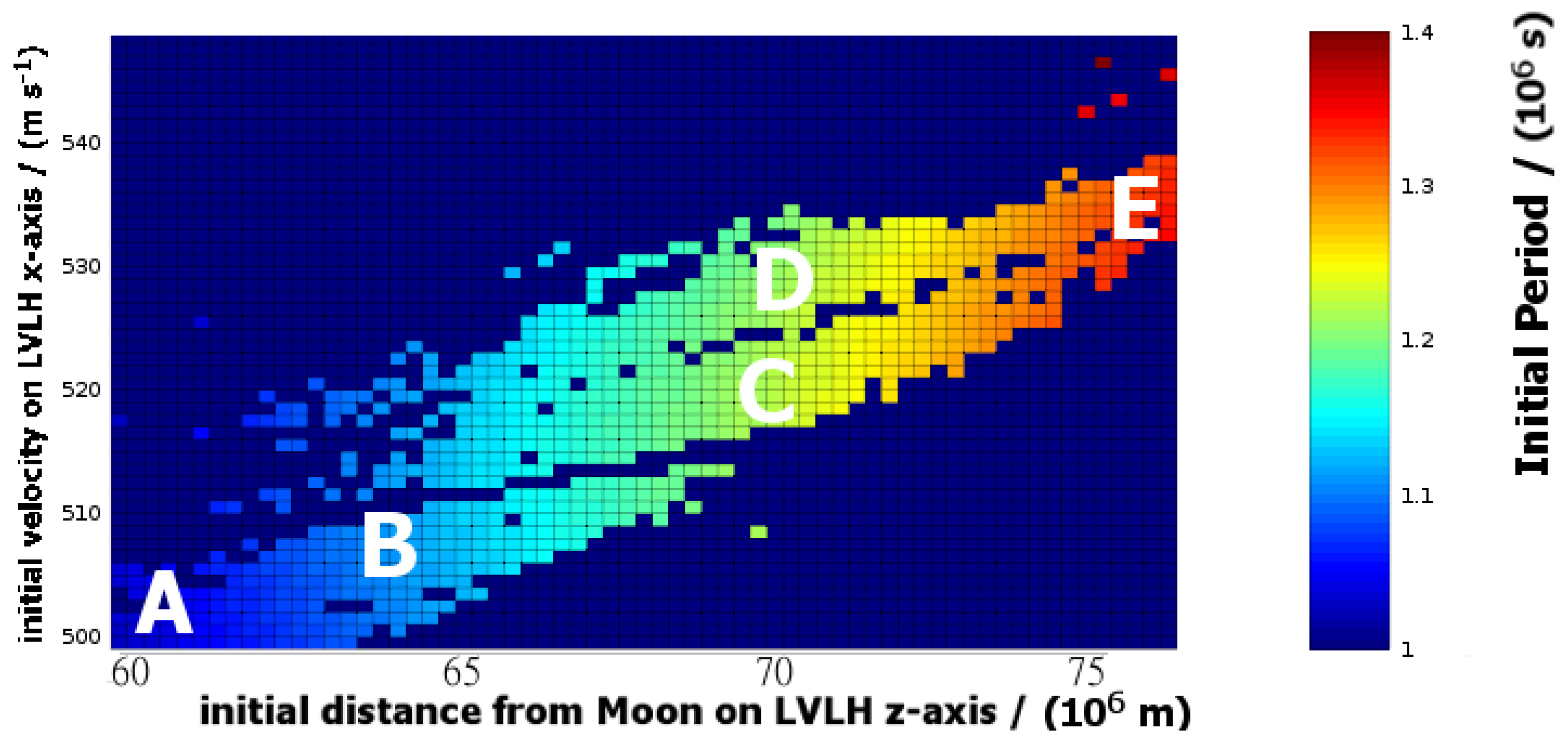
Figure 22.
Detailed view of the initial orbital period, with the color axis in seconds. The data is restricted to those states for which the trajectory will be stable for 30 years.
Figure 22.
Detailed view of the initial orbital period, with the color axis in seconds. The data is restricted to those states for which the trajectory will be stable for 30 years.
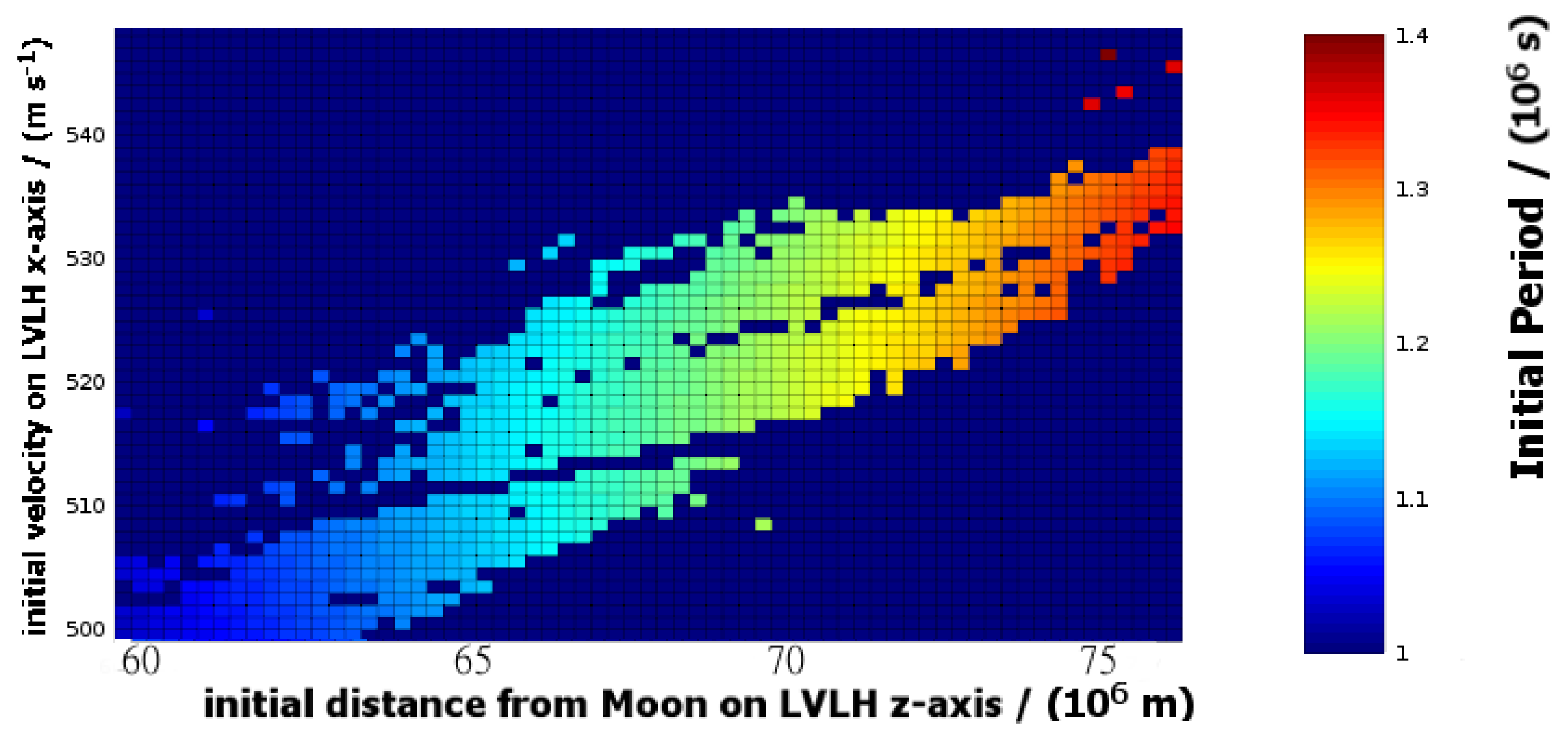
Figure 23.
Detailed view of the final orbital period for the same initial conditions as Figure 22. The color-axis shows the period in seconds.
Figure 23.
Detailed view of the final orbital period for the same initial conditions as Figure 22. The color-axis shows the period in seconds.
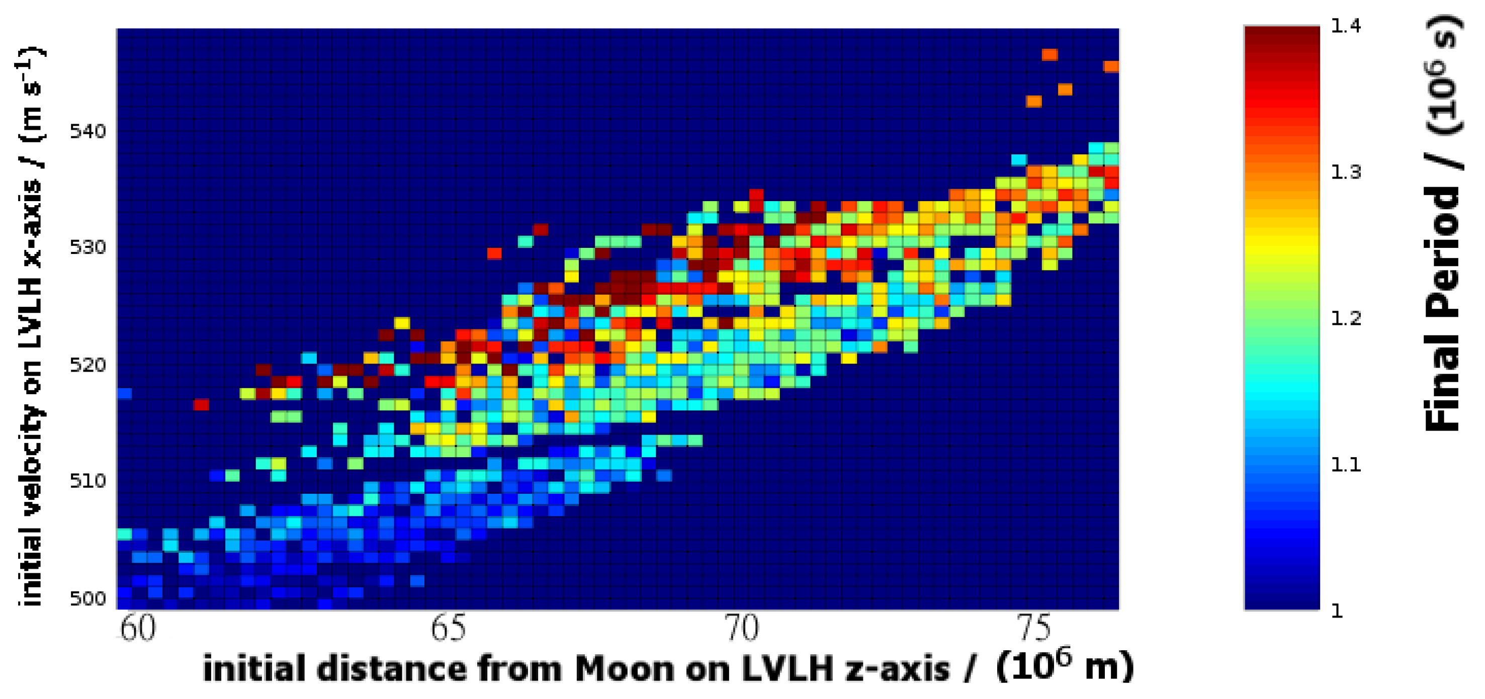
Figure 24.
Detailed view of the mean orbital period for the same initial conditions as Figure 22. The color-axis shows the period in seconds.
Figure 24.
Detailed view of the mean orbital period for the same initial conditions as Figure 22. The color-axis shows the period in seconds.

| Initial Position/ m | Initial Velocity/m·s | Average Period/ s | Period Ratio | Possible Resonance |
|---|---|---|---|---|
| 6.00 | 498 | 1.028 | 2.3 | 3:4:7 |
| 6.45 | 507 | 1.105 | 2.13 | 5:6:11, 7:8:15 * |
| 6.95 | 519 | 1.191 | 2.0 | 1:1:2 |
| 7.075 | 529 | 1.274 | 1.85 | 6:5:11, 7:6;13 * |
| 7.725 | 539 | 1.271 | 1.86 | 6:5:11, 7:6;13 * |
* Lowest order resonances that are close to the observed period ratio. It is unclear whether these are representative of resonant states.
© 2016 by the author; licensee MDPI, Basel, Switzerland. This article is an open access article distributed under the terms and conditions of the Creative Commons Attribution (CC-BY) license (http://creativecommons.org/licenses/by/4.0/).
Share and Cite
MDPI and ACS Style
Turner, G. Results of Long-Duration Simulation of Distant Retrograde Orbits. Aerospace 2016, 3, 37. https://doi.org/10.3390/aerospace3040037
AMA Style
Turner G. Results of Long-Duration Simulation of Distant Retrograde Orbits. Aerospace. 2016; 3(4):37. https://doi.org/10.3390/aerospace3040037
Chicago/Turabian StyleTurner, Gary. 2016. "Results of Long-Duration Simulation of Distant Retrograde Orbits" Aerospace 3, no. 4: 37. https://doi.org/10.3390/aerospace3040037
Note that from the first issue of 2016, this journal uses article numbers instead of page numbers. See further details here.