Multi-UAV Doppler Information Fusion for Target Tracking Based on Distributed High Degrees Information Filters


1
Department of Electrical Engineering, Polytechnique de Montréal, 2900 Boulevard Edouard-Montpetit, Montréal, QC H3T 1J4, Canada
2
Department of Aerospace Measuring and Computing Systems, Saint Petersburg State University of Aerospace Instrumentation, 67 Bolshaya Morskaya, Sankt-Peterburg 190000, Russia
*
Author to whom correspondence should be addressed.
Aerospace 2018, 5(1), 28; https://doi.org/10.3390/aerospace5010028
Submission received: 1 January 2018
/
Revised: 14 February 2018
/
Accepted: 22 February 2018
/
Published: 8 March 2018
(This article belongs to the Collection Unmanned Aerial Systems)
Abstract
:Multi-Unmanned Aerial Vehicle (UAV) Doppler-based target tracking has not been widely investigated, specifically when using modern nonlinear information filters. A high-degree Gauss–Hermite information filter, as well as a seventh-degree cubature information filter (CIF), is developed to improve the fifth-degree and third-degree CIFs proposed in the most recent related literature. These algorithms are applied to maneuvering target tracking based on Radar Doppler range/range rate signals. To achieve this purpose, different measurement models such as range-only, range rate, and bearing-only tracking are used in the simulations. In this paper, the mobile sensor target tracking problem is addressed and solved by a higher-degree class of quadrature information filters (HQIFs). A centralized fusion architecture based on distributed information filtering is proposed, and yielded excellent results. Three high dynamic UAVs are simulated with synchronized Doppler measurement broadcasted in parallel channels to the control center for global information fusion. Interesting results are obtained, with the superiority of certain classes of higher-degree quadrature information filters.
1. Introduction
Previous works have selected the Gauss–Hermite Kalman filter (GHKF) and its information version (GHIF) as the more accurate nonlinear filter for different multi-sensor fusion and target tracking problems, but did not propose any alternative to its high computational complexity and its limited implementation in practice. A special case, when sensors are non-stationary, has not been well investigated, which is assumed in this paper with high-speed dynamic unmanned aerial vehicles (UAVs). It is well-known that GHKFs are impracticable for medium- and high-dimensional systems; the curse of the dimensionality problem existing in the tensor product-based Gauss–Hermite information filter can be elegantly alleviated using the novel seventh-degree cubature information filter derived by authors in [1,2]. In parallel to estimation accuracy and the alleviated computation complexity, the 7th-degree cubature information filter (CIF) has also been tested and analyzed against small and high non-Gaussian measurement noise statistics. In the frame of information space, a modification of the Kalman filter is processed, where the state estimates and their corresponding covariance are replaced by the information matrices and corresponding vectors, respectively, in the information space [3]. The nonlinear filtering problem statement remains the same, but it becomes more attractive in a centralized fusion based on distributed information processing, and is given by the following equations:
In this paper, a 7th-degree and multiple 5th-degree cubature and quadrature information filters are derived and applied to multi-sensor information fusion multi-UAV target tracking. The 5th-degree Gauss–Hermite information filter has clearly demonstrated its superiority to the 5th-degree and 3rd-degree cubature information filters. The seventh-degree cubature information filter (7th degree-CIF) has been demonstrated to be a stronger algorithm with higher precision than previous lower-degree versions such as the fifth- and third-degree cubature Kalman filter (CKF). Nevertheless, it has yielded slightly lower performances compared to the 5th-degree Gauss–Hermite information filter [4,5].
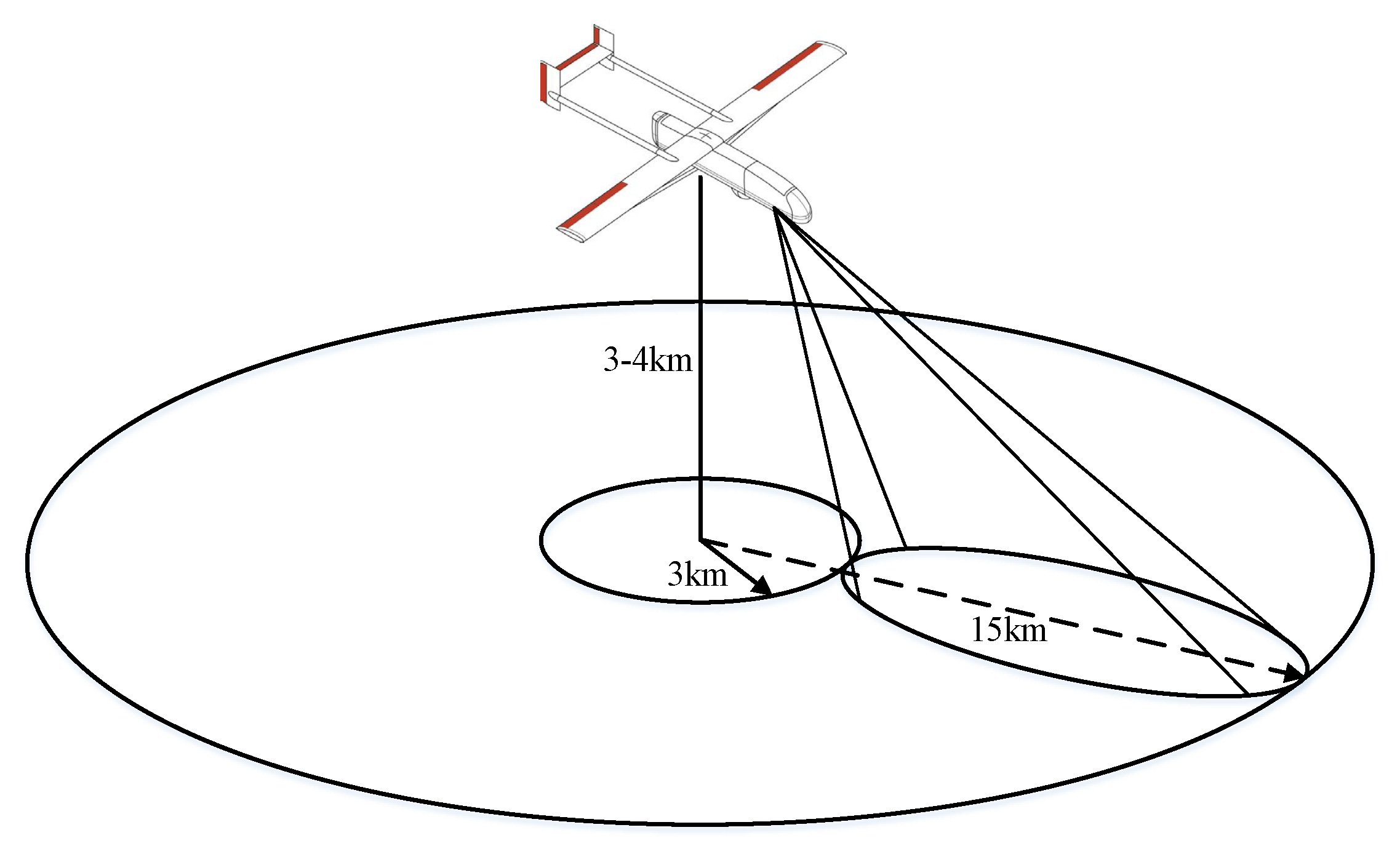
The sensor considered is a pulse-Doppler Radar which produces a measurement vector containing the range, azimuth, elevation, and Doppler; see Figure 1. The Doppler measurement is defined as the target speed in the sensor direction. Doppler radars can measure the component of the velocity of targets toward or away from the radar. Therefore, the Doppler is not expressed as a frequency in Hz, but as a speed in m/s. In this paper, tracking in Cartesian coordinates is considered, for which the state vector contains at least the position and speed in the x, y, and turn rate [6,7].
Remark 1:
The UAV size and class used in our simulation are medium altitude, long-endurance UAS platforms—still smaller than a light aircraft. They usually have a wingspan of about 5–10 m (16–33 feet) and can carry payloads of 100 to 200 kg. It is a very well-adapted size and class for our application when carrying a payload between 50 and 80 kg (Doppler Radar block) [8,9,10,11].
2. Multiple Sensors Modeling
2.1. Doppler Measurement Model
Observation: From the delay and bearing, a direct polar transformation can recover the 2D position. However, the velocity vector is only projected along the radial axis through the Doppler effect (range-rate). It means that multiple measurements and position data storage are needed to unambiguously recover velocity. Before the performance can be analyzed, a performance parameter needs to be defined. For most surveillance Radars, position accuracy is the most important performance parameter.
However, for a target tracking to be efficient for the multi-UAV system, a minimum degree of accuracy in the state estimate is necessary. Therefore, purely analyzing position accuracy is insufficient for this paper. Instead of estimating the accuracy only in range, other measurements such as bearing, elevation, and Doppler need to be taken into account. Below is the measurement signal component from Doppler Radar onboard each UAV:
where is the range from a reference sensor (UAV) to the target, the bearing, and the range rate. By using Taylor series expansion, the linearized measurement matrix is derived from . The Jacobian matrix and its second Hessian matrix of the measurement function h are then obtained, which are required for the implementation of the extended Kalman filter (EKF), second-order EKF, and their respective information space forms.
To investigate the impact of Doppler accuracy on the system performance, the accuracy is increased and decreased, and the system performance is compared to the performance measured in standard conditions defined in the simulation section. In this paper, Doppler range, range rate, and bearing signal are assumed to be observable and used as the measurement sequentially during all simulations. Comparative results are then illustrated and discussed in the last section [12].
2.2. Nonlinear Filtering Problem Statement
Different versions of information filters were developed and designed based on EKF, unscented KF (UKF), and generally called sigma points KFs including EKF, 2nd-order EKF, UKF, central difference KF (CDKF), divided difference KF (DDF), and particle filters as well, such as in the literature [13]. The extended information filter (EIF), its iterative form, a 2nd-order extended information form with its iterative forms were derived, and the cubature information filter was used in [14] to solve the pedestrian integrated navigation problem in a foot-mounted sensor fusion problem. The unscented information filter (UIF) was used for target tracking and derived on the basis of the UKF derived in [15]. As a reply, the third-degree cubature information filter (CIF) was proposed with a square root version by [16].
where and are defined as the quadrature point and the corresponding weight, respectively.
In [16], a new version of a CIF is proposed for pedestrian navigation problems and its superiority is demonstrated compared to UKF/UIF and EKF/EIF previously explored and investigated in the literature and by the authors.
2.3. Multi-Sensor Information Fusion
In this paper, sensors are Doppler Radars onboard UAVs, and different information of bearing, range, and range rate is delivered and broadcasted to the control center for global information filtering implementation. Different algorithms in the literature reflect optimal and suboptimal fusion methods, such as in [17,18].
For this goal, multiple quadratures in the literature were introduced and used as a new Gaussian approximation information filter derivation basis, such as the unscented transform and the Gauss–Hermite quadrature (GHQ) rule, and recently a cubature rule-based Kalman filter of degree 3 with the last derivate high-degree cubature Kalman filter proposed in [19] to approximate the Gaussian weighted integrals in the filtering algorithm, see (4). All new filters solve the Gaussian integral given in (4) using a numerical approximation with two fundamental parameters called points and weights, respectively denoted as and [20,21,22].
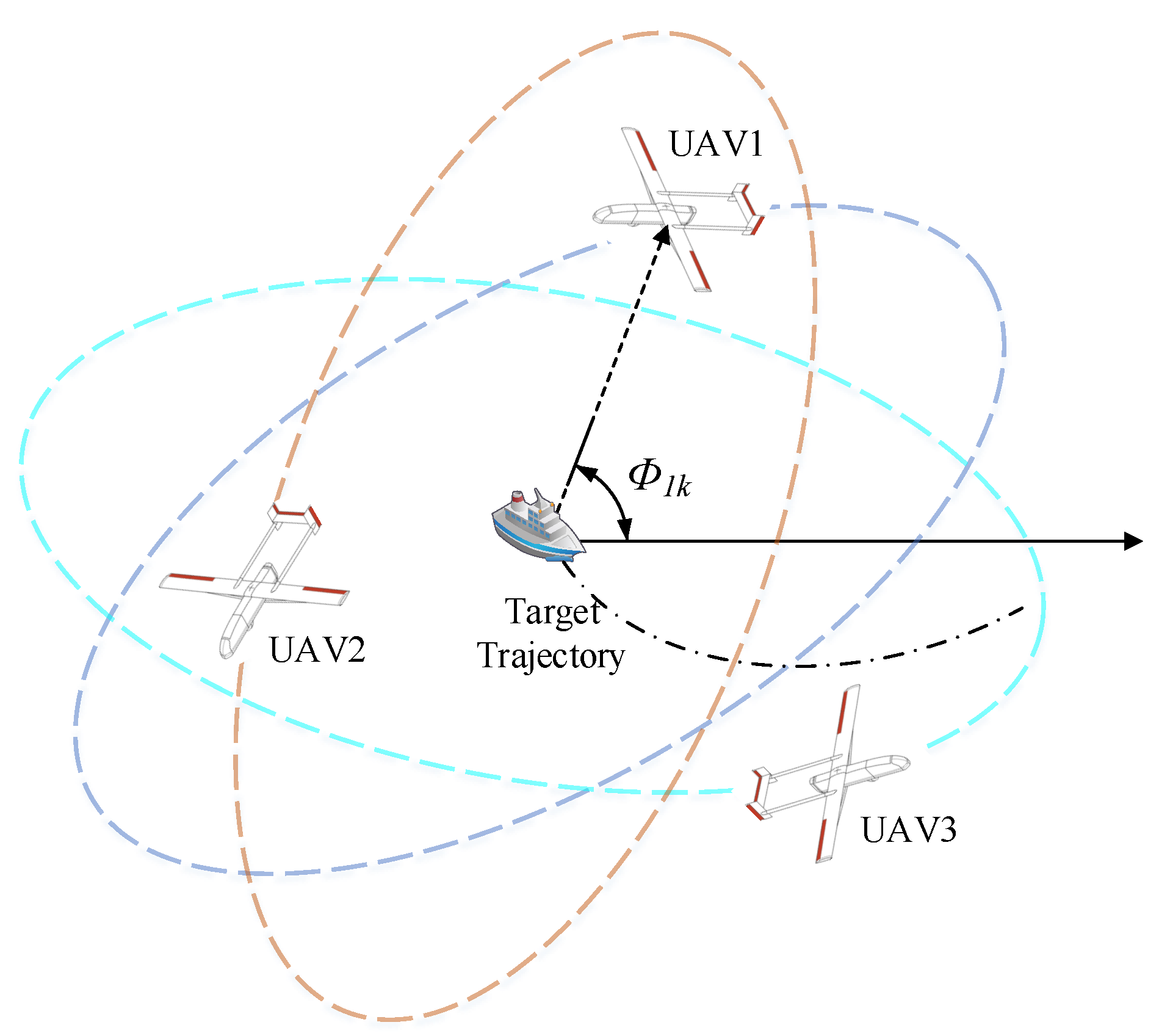
Later in the simulation, we analyse a collaborative target tracking based on a multi-sensor fusion problem statement; sensors are assumed onboard three UAVs in order to track the target manoeuvres. In Figure 2, one can observe the scenario used in the simulation. Multi-UAV navigation, collaboration, and path planning have recently been the subject of investigation; readers can refer to [23,24,25] for a review of trajectory planning and multi-agent algorithms.
2.4. Multiple Quadrature Information Filters
In this paper, instead of developing a Bayesian estimator, four (04) new information filters are proposed, including the major contribution which consists of the derivation of a 7th-degree cubature information filter in addition to Gauss–Hermite information filter of degree 3 and degree 5, and are implemented and discussed in simulations:
- A Gauss–Hermite and 3rd-degree-based KF
- A Gauss–Hermite 5th-degree-based KF
- A varying 5th-degree cubature rules KF—Version 1
- A varying 5th-degree cubature rules KF—Version 2
- A varying 5th-degree cubature rules KF—Version 2
- A kind of 7th-degree cubature rules KF— 7th SSRCKF (7th spherical simplex radial cubature Kalman filter)
For nonlinear filtering and smoothing problems, the algorithms mentioned and listed above are proposed as a superior alternative to CKF and UKF such as in [28]. Even with the innumerous simulation results in different publications that have been carried out with confirmation of the theoretical superiority of high-degree cubature filters, no global criterion exists on how to select the best nonlinear degree cubature Kalman filter. To the best of our knowledge, only their direct application to nonlinear estimation problems has been investigated and proposed. In this paper, we present a generalized quadrature filter algorithm with multiple quadrature point’s generation functions to solve the problem of maneuvering target tracking under time-varying multi-sensor information fusion trajectories (see Figure 3).
The use of mobile and controllable sensing platforms is a relatively new area of research, but it has attracted considerable attention in the generic sensor network literature [29,30]. This type of problem is sometimes referred to as sensor management. The majority of work in sensor management for target tracking assumes one of four practical observation models: range-only, bearing-only, range/bearing, and more recently, range/range-rate with or without bearing, such as proposed in this paper. These observation models are common due to the prevalent use of directional laser and Radar sensors. However, we suppose in this paper that UAVs have heavy fixed wings with high-speed engines, as mentioned in Remark 1 of Section 1.
2.4.1. Gaussian Nonlinear Filters
Based on the different derivation of multiple Gaussian point filters, following the same idea of the authors in [31], one can derive a general form for various quadrature point Kalman filters into a unified algorithm, with the only difference being in how points and weights given in Equation (4) are calculated [31]. Based on Equation (4) notations, and are respectively defined as the quadrature points and corresponding weights. One can use different quadrature, cubature rules, and sigma-points transformation to generate points and weights to be used in the Gaussian filtering algorithm given below. Each algorithm presents some advantages and some limitations. Most of them are discussed in this paper and compared in future sections and in simulations.
2.4.2. Gauss Multiple Quadrature Kalman Filters
It is specified that the following approximated numerical integration methods of the quadrature integral given in Equation (4) are efficient when the process and measurement noises are Gaussian and defined by zero white mean Gaussian noise and covariance and , respectively.
- a
- Initialization:
- Assume at time k that the posterior density function is known. Cholesky factorization can be given as follows:
- b
- Time update:
- c
- Measurement update step:
- The Cholesky factorization , the quadrature points , the predicted measurement , the average prediction , the innovation covariance matrix , the cross-covariance matrix , the quadrature Kalman gain , the state , and the error covariance are updated as follows:
Equations (5)–(19) summarize the general Gaussian quadrature Kalman filter proposed in this paper. A description of time update and measurement update steps at each time step are presented. It is a kind of generalized Gaussian Kalman filter form with multiple quadrature points and associated weight calculation variants. In the next section, one can transform the above equations into the information space framework.
3. Gaussian Points Information Filters Derivation
In the related literature, different versions of information filters were developed, and the only difference with the high-degree information filter proposed in this paper is how to select or how to calculate the quadrature weights and points to approximate a Gaussian integral defined by (4) in Section 2. In this paper, a 7th-degree spherical radial rule-based cubature Kalman filter has been derived as well as a 5th-degree GHIF, on the basis of Mysovskikh formulae of degree seven [32,33], such as developed in a stochastic form previously in the literature. The version we proposed still has a deterministic sampling points algorithm, but provides much better accuracy when compared with previous fifth-degree cubature Kalman filters.
3.1. Sensor Fusion and Selected Approach
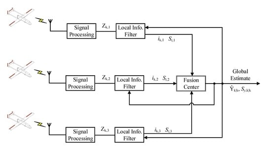
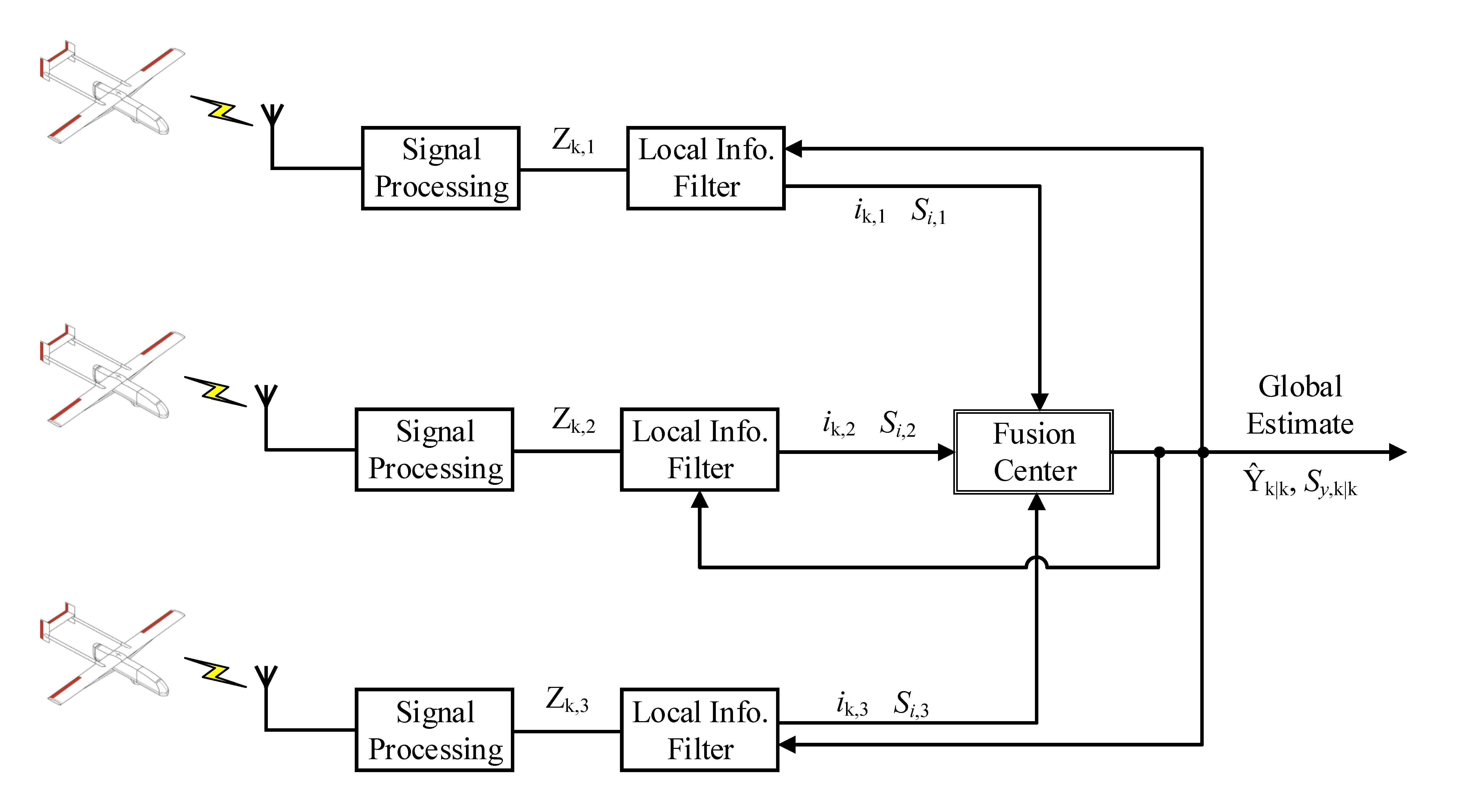
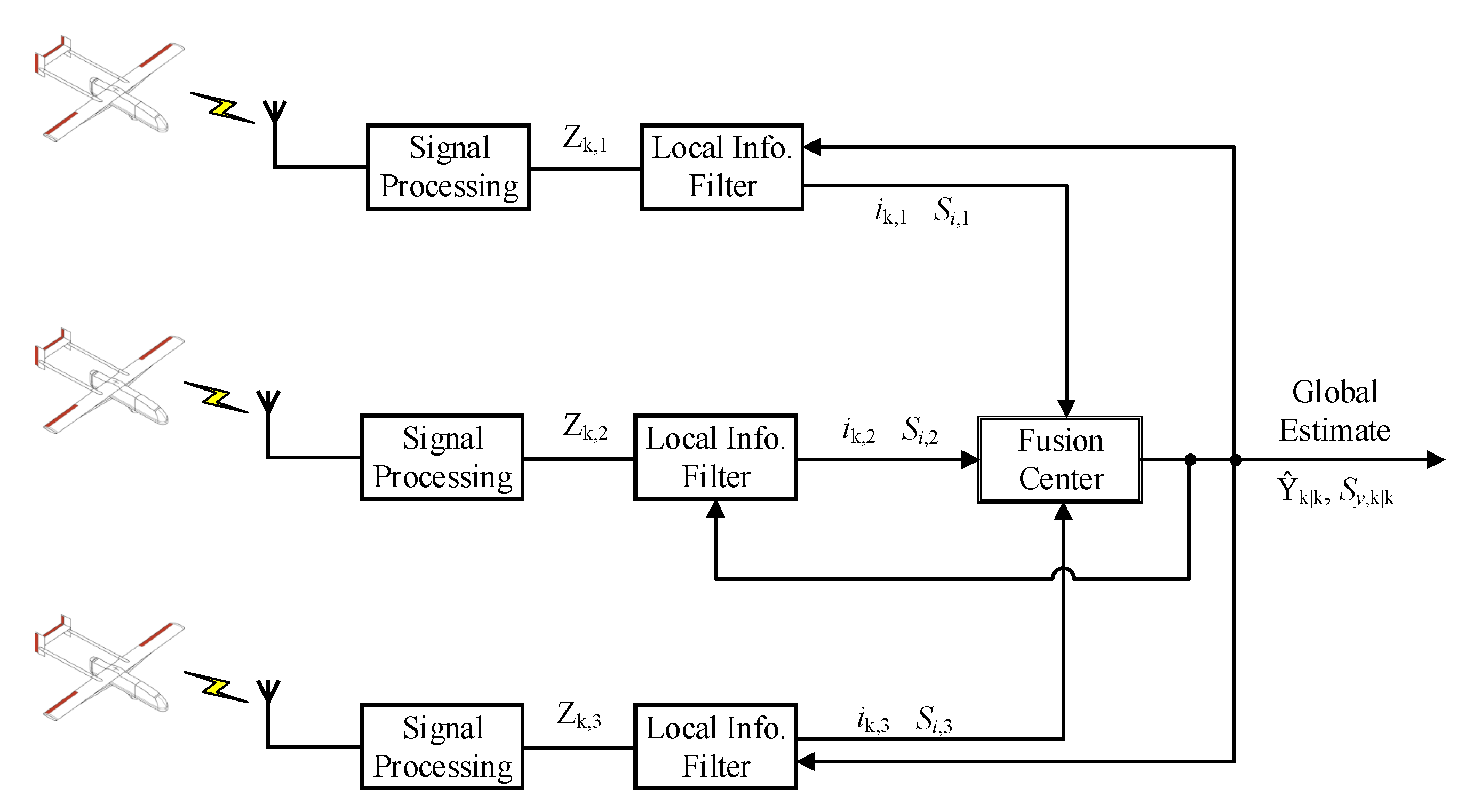
In the sensor fusion literature, there are a number of sensor fusion methods and algorithms based on Kalman and/or information framework, both with their own advantages and drawbacks with centralized and decentralized approaches with their convergence and divergence conditions [34]. In this paper, we specifically consider a distributed configuration with feedback (see Figure 3). In this configuration, when applied to target tracking based on multiple known ground sensors locations (UAV locations), the global estimate is broadcast so that all sensors utilize the global estimate for the next update step in the information filter algorithm. In this paper, moving and maneuvering UAV sensors are assumed to fly at a high speed. It is proposed to implement an information filter instead of the Kalman filter version of the 7th SSRCKF because all sensors’ information, regardless of the number, are simply updated after addition with the same process to compute their covariance, and thus are less computationally consuming, which makes our approach more feasible in real-time operations [34]. Below are equations of information vector and information matrices calculation in the information framework:
- a
- Prediction step:where are the transformed points obtained from the covariance decomposition; i.e.,
- b
- Update step:For multiple-sensor information fusion, the state and the information matrix can be updated by Equations (24) and (25):where is the number of sensors, and are the information state contribution and the information matrix contribution of the mth sensor, respectively. In the EIF framework [5,16], they are defined as:where and are the mth measurement function and the associated Jacobian matrix at time k, respectively; is the covariance of the measurement noise corresponding to the mth measurement equation.
Remark 3:
As described in Equations (26) and (27), it can be seen that the local information contributions of and are only computed at the mth sensor , and the total information contribution including the information state and the information matrix is the simple sum of the local contributions (vectors sum). Thus, one can expect and demonstrate that the information filter is computationally more efficient and well-adapted for multiple-sensor information fusion in a decentralized design than using or deriving the high-degree cubature filter in the Kalman framework.
An important issue in the information we propose is that compared to the extended information filter, the corresponding linearized measurement Jacobian matrix needs to be replaced by the various 5th- and 7th-degree quadrature approximations. However, for the mth sensor, the following equation can be obtained by the linear error propagation:
This is derived using the following steps:
where are the transformed points obtained by the given transformation:
As explained before, and as one can observe, the equation of the information filters remains the analog of the ones presented and proposed for previous derivations of unscented information filters, cubature information filters, and Gauss–Hermite information filter; the main difference (as mentioned in previous sections) is how to calculate quadrature points and their corresponding weights used to approximate the Gaussian integral given in Equation (4). The problem stated and solved in this paper is related to multi-agent cooperative target tracking as described in [35], but the information filter is proposed instead of other techniques proposed previously in order to allow the number of UAVs to extend without limitation and without alleviating the computational complexity. Thus, different quadrature rules and methods could be applied and transformed into the information framework. Other numerical rules could be investigated by interested readers, as given in [36].
3.2. High-Degree Cubature Information Filters
The cubature rule is a numerical rule used to approximate the integral given in Equation (4). Different cubature rules exist and are available in the books of Sobolev, Strood, and Mysovskikh. In the following sections, the description of the most efficient and optimal rules are described.
Algorithm I:
, points
Here, we describe formulae due to Mysovskikh for integration of the integral in Equation (1). As derived and described in [36], Mysovskikh derives a cubature formula for the surface of the sphere, , based on the transformation group of the regular simplex, with vertices:
, . The set of midpoints of the vertices projected onto the surfaces of the sphere is obtained by the given form:
Based on the selection of the cubature points as and and central symmetry as a requirement of the cubature formula, Mysovskikh calculated and described how a 5th-degree formula requiring points may be constructed of the form
then, using Mysovskikh’s degree-5 formula given in [36,37] for integration over the spherical surface, one can obtain:
This cubature formula was implemented for different state nonlinear model estimation, and results were compared with other 5th-degree cubature rules with Gauss–Hermite as the optimal reference.
Algorithm II:
points
As developed and derived in [36,37], without further development and demonstration and just by reference to the authors for deeper theoretical aspects, the second algorithm proposed for nonlinear filtering problems as an improvement of the 3rd-degree cubature Kalman filter derived and developed for filtering and smoothing problems is given below (this formula is shown as reported in [37]):
It was demonstrated in [37] that Algorithm II and Algorithm I allow the achievement of exactly the same result when applied to a radically symmetrical surface.
Algorithm III:
points
Another class of cubature rules with the same number of cubature points based on the work of Sobolev on invariant theory has emerged a class of formulae given in the following and described previously in [37]:
IMPORTANT NOTE: For better understanding of the difference between Algorithm II and III in which cubature points lie on the surface of a sphere with fixed radius (independent of the problem dimension n), it is mentioned that those of Algorithm II lie on a surface that grows with n (as do those of Algorithm I). This means that we have another good criterion connected with efficiency: The efficiency and optimality of the cubature rule depend on the state dimension.
Algorithm IV:
points
This is a formula valid for given by Stroud and reported by authors in [37] (not implemented in this paper).
For the interest of readers and specialized researchers in nonlinear filtering and the derivation of new cubature-based Kalman filtering algorithms, the following values are given on the basis of the form given as reported in [37]. Table 1 reflects the computational time complexity of the proposed filters and cubature rules.
4. Seventh-Fifth Degree Spherical-Radial Rule: Genz–Stroud–Mysovskikh (1981)
In this work, the seventh spherical rule described in [37,38] is considered as the basis of the novel seventh-degree information filter, following the definition of the efficient fifth-degree Mysovskikh cubature rule given in the previous section. The points are projections of the centroids of unit vertex regular n-simplex faces onto . One efficient seventh spherical degree rule given by [37] can be rewritten as below, as in [37]:
The points are projections of the centroids of unit vertex regular n-simplex faces onto . The set of is
The set is given by
The rule uses values.
In [37,38], methods of stochastic rules for the unbounded radial interval and the spherical surface have been combined to give stochastic rules for the original integration region. The general form for a stochastic spherical-radial (SR) rule with a degree l rule for the spherical surface integral and a degree m rule for the radial integral is given in [38]. This method is not applied in this paper, and we have selected the most efficient SR rule of degree seven with one point less that of the stochastic SR rule proposed by the authors in [38]. In the following section, details about how to implement the seventh-degree spherical radial rule in the Gaussian filtering framework are presented.
These proposed formulas were implemented and applied to multiple UAV-based target tracking problems and numerical simulations showing equivalent performances to the third 3rd-degree cubature rules and 5th cubature first formula proposed and derived from the cubature rules developed until the superior degrees seven, nine, etc. Other references in the literature can be found in [38,39]. In Table 2, one can observe the advantage of implementing a 7th-degree CKF instead of third and fifth degree GHKF.
Finally, when replacing the numerical integral given in Equation (44) in the general Gaussian point-based filter algorithm given in Equations (2) and (42), one obtains the new seventh-degree spherical simplex radial cubature Kalman filter (7th SSRCKF) [38]. When comparing the lower bound of the seventh-degree cubature rule with the one which is proposed and other seventh-degree forms proposed in the literature, the 7th SSRCKF is more efficient according to the number of points, with only cubature points. In Figure 4, it is easy to observe the difference between GHKF and multiple high-degree CKFs. So, the proposed rule approaches the lower bound given by . The proposed solution for the derivation of the new information filter of degree seven is more efficient than the existing similar degree rules in the literature (see Figure 4).
5. Simulation
The simulation is based on 100 Monte-Carlo runs for all scenarios including range/range rate and bearing-only tracking models. The metric used to compare the performance of the information filters is the root mean square error (RMSE). The target dynamics is highly nonlinear due to the unknown turn rate. It has been used as a benchmark to test the performance of different nonlinear filters [22,23,24]. The discrete-time dynamic equation of the target motion is given by:
where , , and are the position and velocity at time k, respectively. In this section, the performance of multiple quadrature-based information filters is demonstrated via a benchmarking of target-tracking problem with time-varying Gaussian measurement noises, which is to track a target executing a maneuvering turn in a two-dimensional space with unknown and time-varying turn rate done in this paper. In this section, the new proposed seventh-degree spherical simplex radial CIF is applied, three novel variant fifth-degree CIFs, higher-degree CIF, and high-degree GHIFs are also considered for the tracking of multiple moving sensors. The dynamic equation of this tracking problem is highly non-linear due to the unknown turn rate. In this simulation, we have considered a problem with [range, range rate, bearing] information in order to demonstrate the efficiency of the proposed approaches and methods in the information space.
Remark 4:
We assume each UAV is equipped with highly accurate integrated navigation system INS (Inertial Navigation System)/GPS (Global Positioning System) with ultra-tightly-coupled architecture, very well known to be robust against jamming and denied GNSS (Global Navigation Satellite System) environment; see [40,41]. Note that during simulations, positions of UAVs were assumed known with errors within the range of 2.5–5 m.
5.1. Multi-UAVs Range-Rate-Only Target Tracking
We considered the problem of range rate tracking assuming that there were three (03) moving sensors in known locations, fixed without uncertainties; other problem statements can be found, for example, in [39,42]. In the first simulation, three sensors are used to measure the range rate between the target and the sensors. The measurement sampling interval was = 0.1 s, then switched to 0.5 s. The simulation results are based on 100 Monte Carlo runs. The initial estimate values with different uncertainty level values were introduced gradually. They are given as follows: = [1000 m, 300 m/s, 1000 m, 0, −3 deg/s]T and being the initial covariance: . The metrics used to compare the performance of various filters was the root mean square error (RMSE). The Doppler measurement is described in Equation (2).
Different covariance noise values were assigned to each component of the measurement vector. Range, range rate, and bearing were simulated with appropriate values. Illustrations are given in Figure 5, Figure 6 and Figure 7. See Figure 6 for comparative results of the target trajectory estimation using different nonlinear filters proposed in this paper.
5.1.1. Extended Results for Range Rate Doppler Tracking
Through these simulations, one can construct different assumptions on what will be the trajectory model of the target after time Ts (tracking simulation time). Trajectory fitting was applied to the estimated trajectory in order to predict the next maneuver and build appropriate interactive multiple models based on fitting trajectory generation: spline, cubic, quadric, etc. An interpretation of the multiple hypothesis trajectories could be that the multi-UAV shall be assigned new tracking tasks on the basis of trajectory model instead of velocity and turn rate model. See Figure 8 for a clear description of the simulated scenario in this paper.
5.1.2. Range Rate Observation
From Figure 5, Figure 6, Figure 7 and Figure 8, one can observe the superiority of the 5th-degree GHIF, 5th-degree and 7th-degree CIF compared to other high-degree cubature information filters. In general, range rate maintained good estimation results when three UAVs were constantly moving around the target trajectory. However, it must be specified that the multi-UAV location is known exactly. The simulation conditions are as follows:
Integration time = 0.1; State dimension n = 5; Initial turn rate = −3/(); Simulation duration = 100; reptimes = 100; Monte Carlo samples N = 100; Process noise covariance’s values: q1 = 0.1; q2 = 1.75 × 10.
5.2. Multi-UAVs Range-Only Target Tracking
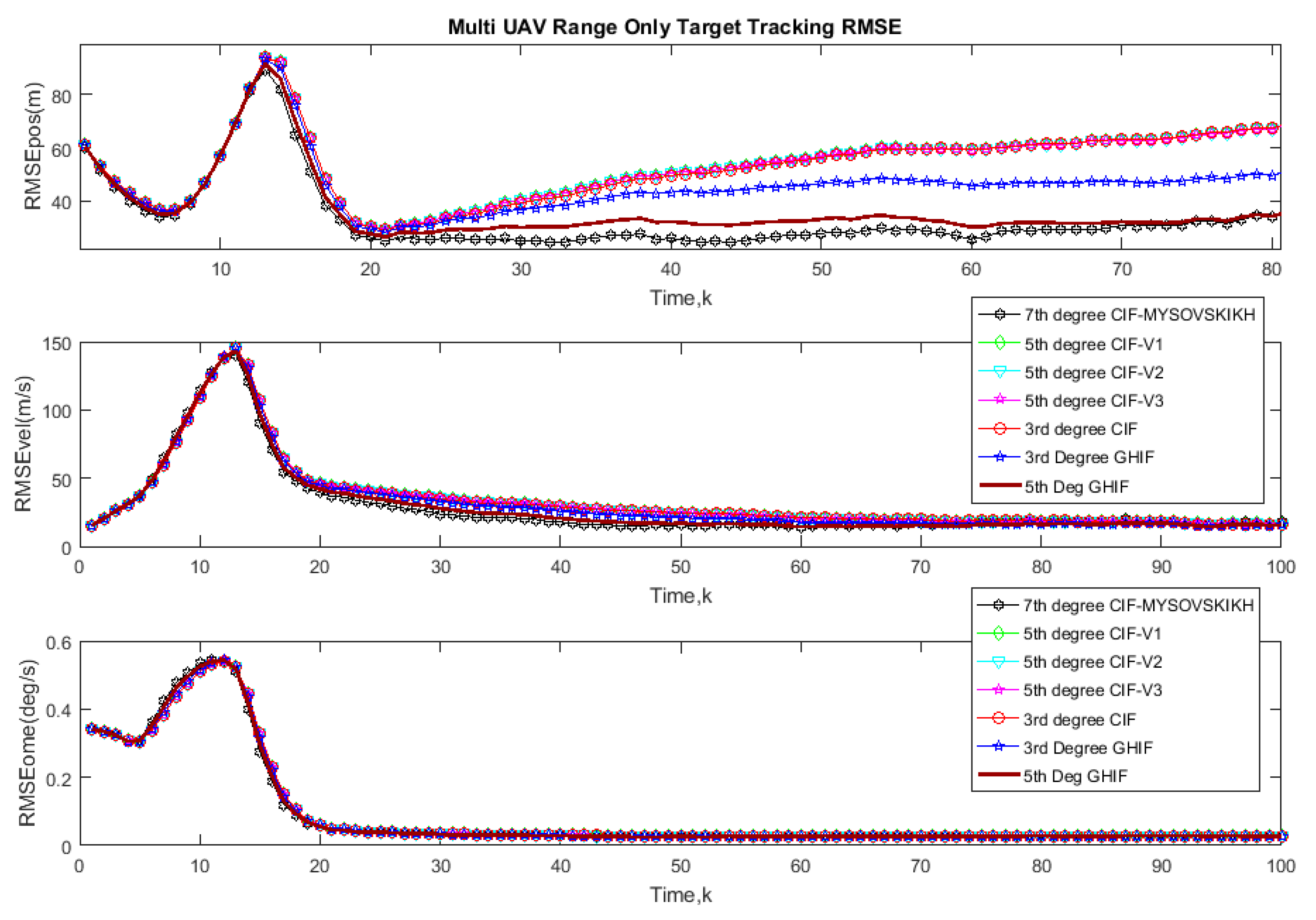
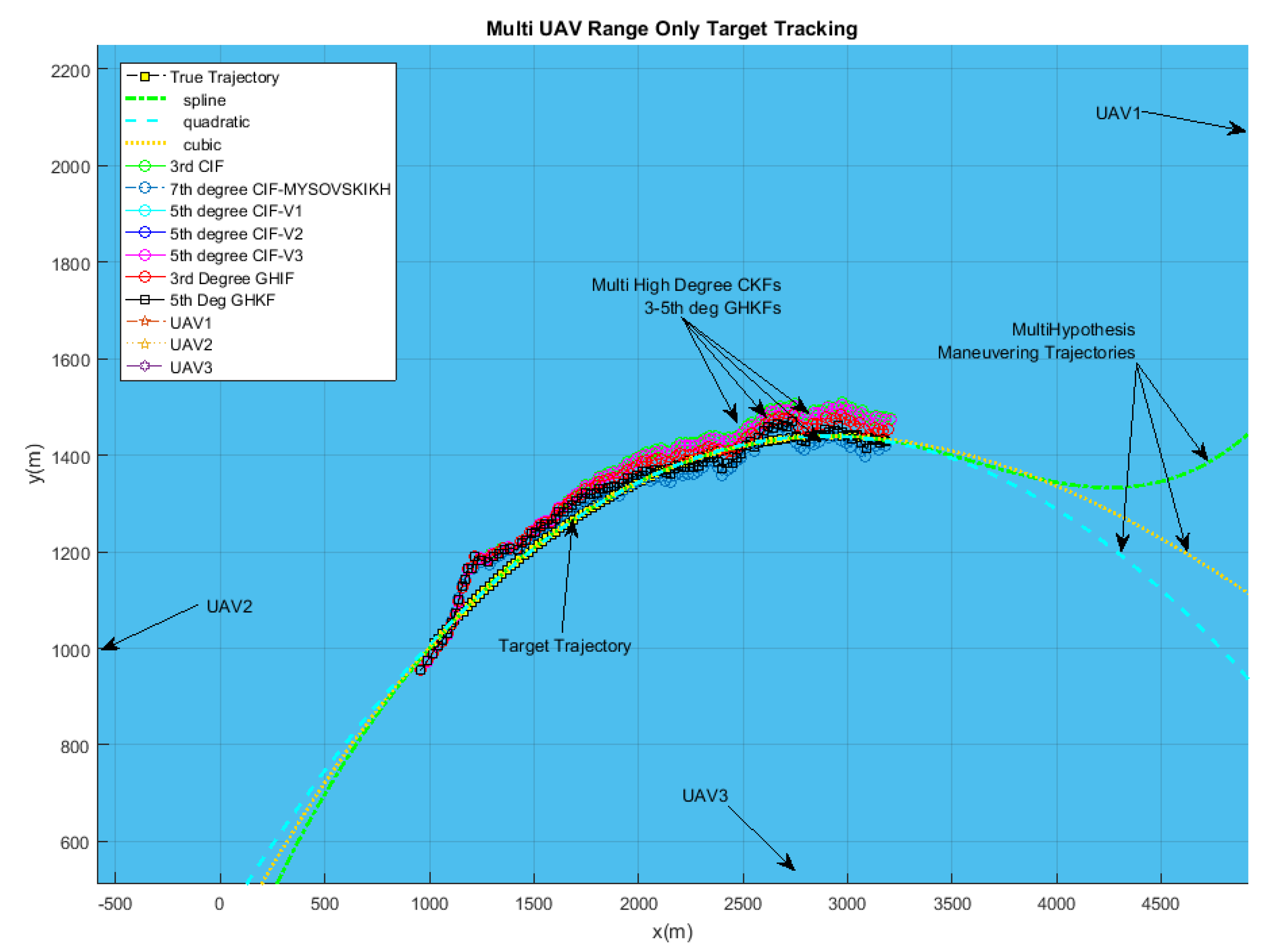
In the case of Multi-UAVs range-only target tracking, from Figure 9, Figure 10, Figure 11 and Figure 12, it is interesting to observe and confirm the superiority of the 5th-degree GHIF, 5th-degree and 7th-degree CIF compared to other high-degree cubature information filters. This can be explained by the degree of nonlinearity in the measurement equation. Multi-UAVs range-only target tracking maintains a good estimation accuracy. UAVs are flying in the same scenario, such as for range rate simulation. Initial conditions and parameters values are exactly the same.
5.3. Discussion
During these simulations, different measurements from each UAV were used to compute the local innovation matrix and broadcasted to the control center for global computing information. In our scenarios, we had three (03) UAVs in operation of Search and Rescue and tracking a target in a configuration where there was no leader. We supposed that positions and local speeds of UAVs were known, which were accurate enough to achieve better performances during the tracking mission. One can observe, however, that from range rate to range-only tracking and compared with previous bearing simulation results, the accuracy and performances of the information filters proposed and derived for this problem are different, and show interesting results. For instance, in this paper there is no attention given to leader–follower formation criteria or a rendezvous point path planning for the multi-UAVs using Dubins method and other approaches [43].
We repeated exactly the same simulation conditions for different scenarios using range rate, range-only, and bearing-only tracking for coherent benchmarking between different filtering methods and new high-degree derivation. It is clear after analyzing the results in Figure 5, Figure 6, Figure 7, Figure 8, Figure 9, Figure 10, Figure 11 and Figure 12 that higher disturbances and errors affect the target trajectory estimation performances for all categories of filters in the case of range-only tracking; on the contrary, in the range rate measurement availability, higher accuracy, and lower error were achieved and maintained, especially for the seventh-degree CIF and the fifth-degree GHIF. Future work will consider multiple Doppler measurements affected by non-Gaussian noises modeled as in [44] with divergence avoidance algorithms development such as in [45].
6. Conclusions
In this paper, a new class of fifth- and novel seventh spherical radial-degree CIFs are proposed for multiple sensors’ information fusion based on Mysovskikh’s efficient 7th-degree spherical rule. An accurate and efficient Gauss–Hermite quadrature information filter has been applied as a lower bound for performance evaluation of the proposed methods. The influence of observation condition and the availability of different measurements have been demonstrated and carried out. In this paper, a centralized but distributed information filtering-based method improved the performances of the multi-sensor target tracking algorithm when derived in the information space. This new robust and efficient information filter has greatly improved the performances in different scenarios and configurations, with range-only, range rate, and bearing-only tracking conditions. Besides the theoretical formulation and the proposal of the recently-developed high-degree information filters, new results have been illustrated and discussed considering this problem of multi-UAV target tracking using different Doppler measurements.
All of the algorithms we implemented on an Intel CoreTM i3-2120, 3.30 GHZ CPU with 4.00 Gb RAM. Table 2 shows the number of points and computational time of CKF, 5th CKF-V1, 5th CKF-V2, 5th CKF-V3, and 7th CKF for each run. The points of the 5th-degree-CKF-V1 as well as the 5th-degree-CKF-V2 and 5th-degree-CKF-V3 differed only by few points. As shown in Table 2, the computational time of the algorithms is approximately proportional to the number of points. One can observe that the computational cost of the multiple fifth-degree CKFs (V1, V2, and V3) is slightly different from each other due to the different 5th-degree cubature rules. Due to the computation complexity of information, the 7th SSRCKF algorithm is larger than fifth-degree CKF (V1, V2 and V3), but can be implemented onboard UAVs with fast CPU boards. It is also important to mention that the advantages of the use of the high-degree cubature filters are that the points and weights of the numerical integration are calculated offline.
An attractive problem of rendezvous point selectivity during Search and Rescue (SAR) missions and leader–follower algorithm development for this specific matter should be in the scope of interest and certainly considered as a challenging problem statement. For future works and presently under development, a stochastic form of the seventh-degree cubature Kalman filter will be applied to denser moving sensor networks with large uncertainties not only at the initialization step but also in the Doppler measurement covariance and sensor location information. Experimental work is already in an advanced stage based on the work of our co-worker [46] for field tests onboard UAVs.
Finally, optimal dynamical sensors placement based on Fisher information matrix based on novel interpolation seventh-degree cubature rules described by Misovskikh in [47] is being developed and implemented and will be proposed in future work as a superior alternative based on deterministic and stochastic sampling methods. In the future, we plan to implement our algorithms and install Doppler radars prototypes onboard a real fixed wing UAVs during remote sensing missions in the arctic for validation purposes.
Acknowledgments
This work was supported by Ministry of Education and Science of the Russian Federation Grant No. 9.1559.2017, Russian Foundation for Basic Research Grant 18-08-00234, Russian Science Foundation Grant 16-19-10381, and Postdoctoral Fellowship of the 10th GERAD competition.
Author Contributions
Hamza Benzerrouk performed simulations and organized the paper content and wrote the paper; Alexander Nebylov has verified the feasibility of the theoretical approaches proposed in this paper with multiple clarifications. Meng Li contributed to improving the paper in terms of formulation, simulation, and grammar.
Conflicts of Interest
The authors declare no conflict of interest.
References
- Jia, B.; Xin, M.; Pham, K.; Blasch, E.; Chen, G. Multiple Sensor Estimation Using A High-Degree Cubature Information Filter. In Proceedings of the SPIE Defense, Security, and Sensing 2013, Baltimore, MD, USA, 29 April–3 May 2013. [Google Scholar]
- Jia, B.; Xin, M.; Cheng, Y. High-degree cubature Kalman filter. Automatica 2012, 49, 510–518. [Google Scholar] [CrossRef]
- Benzerrouk, H.; Nebylov, A.; Salhi, H. Contribution in Information Signal Processing for Solving State Space Nonlinear Estimation Problems. J. Signal Inf. Process. 2013, 4, 375–384. [Google Scholar] [CrossRef]
- Jia, B.; Xin, M. Multiple sensor estimation using a new fifth-degree cubature information filter. Trans. Inst. Meas. Control 2015, 37, 15–24. [Google Scholar] [CrossRef]
- Jia, B.; Xin, M.; Cheng, Y. Multiple sensor estimation using the sparse Gauss-Hermite quadrature information filter. In Proceedings of the American Control Conference (ACC 2012), Montreal, QC, Canada, 27–29 June 2012; pp. 5544–5549. [Google Scholar]
- Elling, L. Analysis of Interacting Multiple Model-extended Kalman Filters at High Update Rates; Nederlandse Defensie Academie: Den Haag, The Netherlands, 2015. [Google Scholar]
- Ahmed, M.; Subbarao, K. Target Tracking in 3-D Using Estimation Based Nonlinear Control Laws for UAVs. Aerospacee 2016, 3, 5. [Google Scholar] [CrossRef]
- Schwartz, C.E.; Bryant, T.G.; Cosgrove, J.H.; Morse, G.B.; Noonan, J.K. A Radar for Unmanned Air Vehicles. Linc. Lab. J. 1990, 3, 119–143. [Google Scholar]
- Göktoǧan, A.H.; Brooker, G.; Sukkarieh, S. A compact millimeter wave Radar sensor for unmanned air vehicles. Field Serv. Robot. 2006, 24, 311–320. [Google Scholar]
- Ren, X.; Qin, Y.; Qiao, L. A novel 3D imaging method for airborne downward-looking sparse array SAR based on special squint model. Int. J. Antennas Propag. 2014, 2014, 982014. [Google Scholar] [CrossRef]
- Watts, A.C.; Ambrosia, V.G.; Hinkley, E.A. Unmanned aircraft systems in remote sensing and scientific research: Classification and considerations of use. Remote Sens. 2012, 4, 1671–1692. [Google Scholar] [CrossRef]
- Mittermaier, T.J.; Siart, U.; Eibert, T.F.; Bonerz, S. Extended Kalman Doppler tracking and model determination for multi-sensor short-range Radar. Adv. Radio Sci. 2016, 14, 39–46. [Google Scholar] [CrossRef]
- Julier, S.J.; Uhlmann, J.K.; Durrant-Whyte, H.F. A new method for the nonlinear transformation of means and covariances in filters and estimators. IEEE Trans. Autom. Control 2000, 45, 477–482. [Google Scholar] [CrossRef]
- Benzerrouk, H.; Nebylov, A.; Salhi, H.; Closas, P. MEMS IMU/ZUPT Based Cubature Kalman Filter Applied to Pedestrian Navigation System. Conference Proceedings Paper–Sensors and Applications 2014. Available online: http://sciforum.net/conference/ecsa-1/paper/2395/download/manuscript.pdf (accessed on 1 June 2014).
- Lee, D.J. Nonlinear estimation and multiple sensor fusion using unscented information filtering. IEEE Signal Process Lett. 2008, 15, 861–864. [Google Scholar] [CrossRef]
- Benzerrouk, H. Modern Approaches in Nonlinear Filtering Theory Applied to Original Problems of Aerospace Integrated Navigation Systems with non-Gaussian Noises; Saint Petersburg State University: Sankt-Peterburg, Russia, 2014. [Google Scholar]
- Arasaratnam, I.; Haykin, S. Cubature Kalman Filtering. IEEE Trans. Autom. Control 2009, 54, 1254–1269. [Google Scholar] [CrossRef]
- Sarkka, S.; Hartikainen, J. On Gaussian optimal smoothing of nonlinear state space models. IEEE Trans. Autom. Control 2010, 55, 1938–1941. [Google Scholar] [CrossRef]
- Jia, B.; Xin, M. High-degree cubature joint probabilistic data association information filter for multiple sensor multiple target tracking. In Proceedings of the 53rd IEEE Conference on Decision and Control, Los Angeles, CA, USA, 15–17 December 2014; pp. 304–309. [Google Scholar]
- Dobrodeev, L.N. Cubature Rules with Equal Coefficients for Integrating Functions with Respect to Symmetric Domains. Comput. Math. Math. Phys. 1979, 18, 27–34. [Google Scholar] [CrossRef]
- Mysovskikh, I.P. The approximation of multiple integrals by using interpolatory cubature formulae. In Quantitative Approximation; Devore, R.A., Scherer, K., Eds.; Academic Press: New York, NY, USA, 1980; pp. 217–243. [Google Scholar]
- Genz, A.; Monahan, J. A Stochastic Algorithm for High Dimensional Multiple Integrals over Unbounded Regions with Gaussian Weight. J. Comp. Appl. Math 1999, 112, 71–81. [Google Scholar] [CrossRef]
- Lanillos, P.; Gan, S.K.; Besada-Portas, E.; Pajares, G.; Sukkarieh, S. Multi-UAV target search using decentralized gradient-based negotiation with expected observation. Inf. Sci. 2014, 282, 92–110. [Google Scholar] [CrossRef]
- Jamieson, J.; Biggs, J. Path Planning Using Concatenated Analytically-Defined Trajectories for Quadrotor UAVs. Aerospace 2015, 2, 155–170. [Google Scholar] [CrossRef] [Green Version]
- Chahl, J. Unmanned Aerial Systems (UAS) Research Opportunities. Aerospace 2015, 2, 189–202. [Google Scholar] [CrossRef]
- Cai, W.; Zhang, M.; Zheng, Y.R. Task Assignment and Path Planning for Multiple Autonomous Underwater Vehicles Using 3D Dubins Curves. Sensors 2017, 17, 1607. [Google Scholar] [CrossRef] [PubMed]
- Itkin, M.; Kim, M.; Park, Y. Development of Cloud-Based UAV Monitoring and Management System. Sensors 2016, 16, 1913. [Google Scholar] [CrossRef] [PubMed]
- Lu, J.; Darmofal, D.L. Higher-dimensional integration with Gaussian weight for applications in probabilistic design. SIAM J. Sci. Comput. 2005, 2, 613–624. [Google Scholar] [CrossRef]
- Olfati-Saber, R. Distributed Kalman filtering for sensor networks. In Proceedings of the 46th IEEE Conference on Decision and Control, New Orleans, LA, USA, 12–14 December 2007. [Google Scholar]
- Closas, P.; Prades, C.F.; Vails, J.V. Multiple quadrature Kalman filtering. IEEE Trans. Signal Process. 2012, 60, 6125–6137. [Google Scholar] [CrossRef]
- Sobolev, S.L. Cubature formulas on the sphere invariant under finite groups of rotations. Dokl. Akad. Nauk SSSR 1962, 146, 310–313. [Google Scholar]
- Stoyanova, S.B. Cubature formulae of the seventh degree of accuracy for the hypersphere. J. Comput. Appl. Math. 1997, 84, 15–21. [Google Scholar] [CrossRef]
- George, D.E.; Unnikrishnan, A. On the divergence of information filter for multi sensors fusion. Inf. Fusion 2016, 27, 76–84. [Google Scholar] [CrossRef]
- Heredia, G.; Caballero, F.; Maza, I.; Merino, L.; Viguria, A.; Ollero, A. Multi-Unmanned Aerial Vehicle (UAV) Cooperative Fault Detection Employing Differential Global Positioning (DGPS), Inertial and Vision Sensors. Sensors 2009, 9, 7566–7579. [Google Scholar] [CrossRef] [PubMed]
- Hu, J.; Xie, L.; Xu, J.; Xu, Z. Multi-Agent Cooperative Target Search. Sensors 2014, 14, 9408–9428. [Google Scholar] [CrossRef] [PubMed]
- Zhang, Y.; Huang, Y.; Li, N.; Zhao, L. Interpolatory cubature Kalman filters. IET Control Theory Appl. 2015, 9, 1731–1739. [Google Scholar] [CrossRef]
- Meng, Z.; Luo, Z. Constructing cubature formulae of degree 5 with few points. J. Comput. Appl. Math. 2013, 237, 354–362. [Google Scholar] [CrossRef]
- Zhang, Y.; Huang, Y.; Wu, Z.; Li, N. Seventh-degree spherical simplex-radial cubature Kalman filter. In Proceedings of the 33rd Chinese Control Conference, Nanjing, China, 28–30 July 2014. [Google Scholar]
- Meng, D.; Miao, L.; Shao, H.; Shen, J. A Seventh-Degree Cubature Kalman Filter. Asian J. Control 2018, 20, 250–262. [Google Scholar] [CrossRef]
- Kou, Y.; Zhang, H. Sample-wise aiding in GPS/INS ultra-tight integration for high-dynamic, high-precision tracking. Sensors 2016, 16, 519. [Google Scholar] [CrossRef] [PubMed]
- Bischof, C.; Schön, S. Vibration detection with 100 Hz GPS PVAT during a dynamic flight. Adv. Space Res. 2017, 59, 2779–2793. [Google Scholar] [CrossRef]
- Salamat, B.; Tonello, A.M. Stochastic Trajectory Generation Using Particle Swarm Optimization for Quadrotor Unmanned Aerial Vehicles (UAVs). Aerospace 2017, 4, 27. [Google Scholar] [CrossRef]
- Kikutis, R.; Stankunas, J.; Rudinskas, D.; Masiulionis, T. Adaptation of Dubins Paths for UAV Ground Obstacle Avoidance When Using a Low Cost On-Board GNSS Sensor. Sensors 2017, 17, 2223. [Google Scholar] [CrossRef] [PubMed]
- Benzerrouk, H. Gaussian vs. Non-Gaussian noise in inertial/GNSS integration. GNSS Solut. Inside GNSS Mag. 2012, 32–39. [Google Scholar]
- Schlee, F.H.; Standish, C.J.; Toda, N.F. Divergence in the Kalman filter. AIAA J. 1967, 5, 1114–1120. [Google Scholar] [CrossRef]
- Li, W.; Zhang, H.; Osen, O.L. A UAV SAR Prototype for Marine and Arctic Application. In Proceedings of the ASME 36th International Conference on Ocean, Offshore and Arctic Engineering, Trondheim, Norway, 25–30 June 2017. [Google Scholar]
- Mysovskikh, I.P. Interpolatory Cubature Formulas; Nauka: Moscow, Russia, 1981. (in Russian) [Google Scholar]
Figure 1.
The unmanned aerial vehicle (UAV) Radar has a wide area of 360 deg Field of View (FOV), Radar antenna sweeps out an annular of 3–15 km. Doppler Radar is designed for the automatic detection and tracking of moving ground and marine vehicles as well as low-altitude (maximum altitude: 3–4 km) slow-flying aircraft such as general aviation aircrafts, and helicopters out to a range of 15 km.

Figure 2.
Multi-UAVs-based target tracking problem configuration at time . In this paper, three (03) UAVs are assumed to navigate independently following different circular and elliptical trajectories around the manoeuvring target with high-speed dynamic between 140 and 180 m/s.
Figure 2.
Multi-UAVs-based target tracking problem configuration at time . In this paper, three (03) UAVs are assumed to navigate independently following different circular and elliptical trajectories around the manoeuvring target with high-speed dynamic between 140 and 180 m/s.

Figure 3.
During a search and rescue (SAR) mission, multiple UAVs track a target with centralized distributed measurement information broadcasted to the control center (CC) for information estimate implementation. In this configuration, communication is allowed between each UAV and the CC.
Figure 3.
During a search and rescue (SAR) mission, multiple UAVs track a target with centralized distributed measurement information broadcasted to the control center (CC) for information estimate implementation. In this configuration, communication is allowed between each UAV and the CC.

Figure 4.
Target tracking estimation using 3rd degree CIF, 5th degree CIF-V1-V2-V3 and 7th-degree Cubature Information filters (CIFs) compared to 3rd-degree Gauss–Hermite information filter. UAV1, UAV2 and UAV3 are delivering Doppler measurement information to the control center for global information fusion.
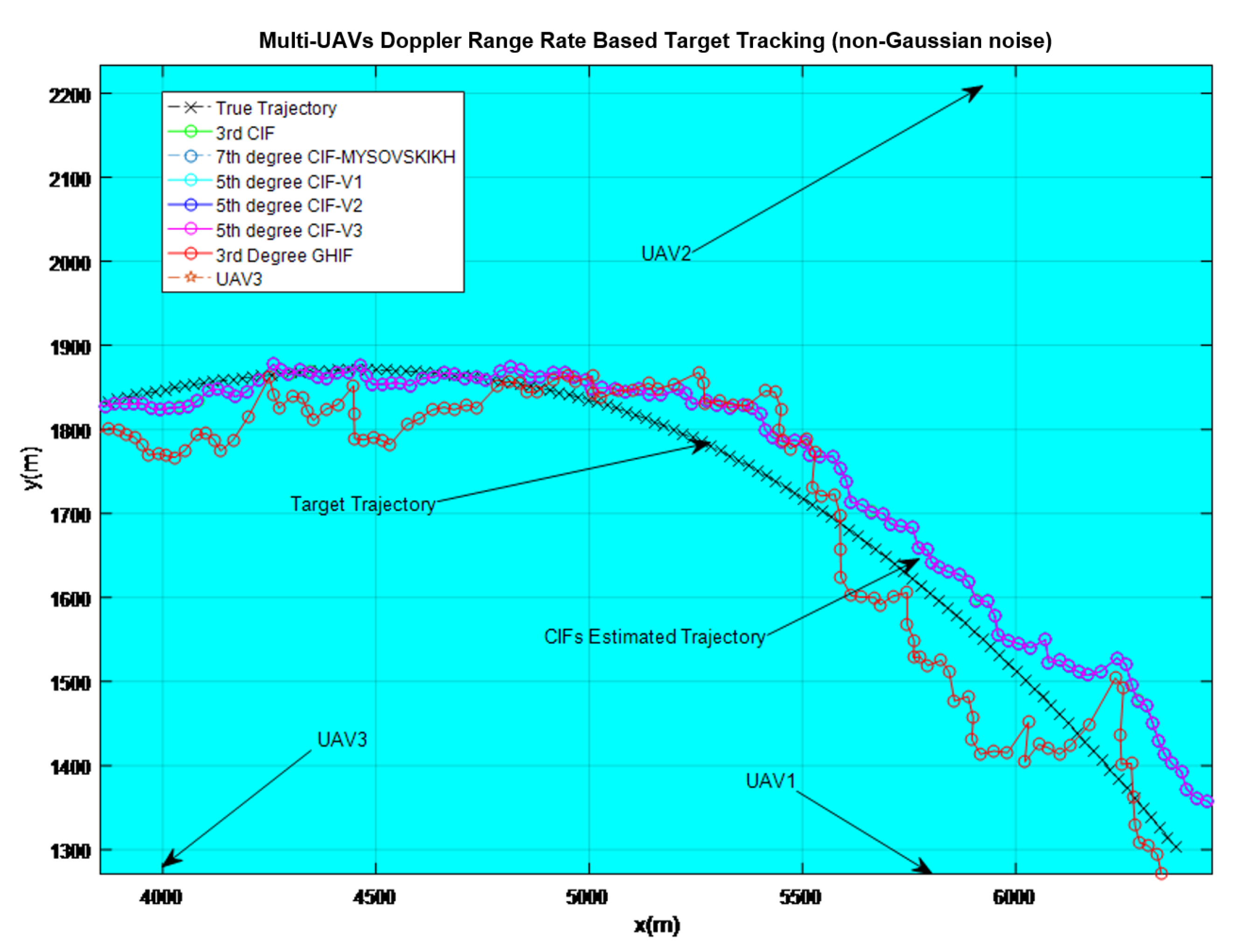
Figure 5.
Range rate Doppler-based estimation: UAV1, UAV2, UAV3 trajectories are clearly described and indicated around the target trajectory. In black, 7th-degree CIF and 5th-degree GHIF are close to the true target trajectory, 5th-degree CIFs and 3rd-degree CIF-GHIF are superposed in pink color with light deviation from the black trajectory estimate. Three possible fitting trajectories (spline, quadric, cubic) are illustrated with discontinuous green, blue, and yellow colors.

Figure 6.
Range rate Doppler-based estimation: Results of 7th-degree CIF, 5th-degree CIF, 5th-degree GHIF, 3rd-degree GHIF compared to the true trajectory in green color.
Figure 6.
Range rate Doppler-based estimation: Results of 7th-degree CIF, 5th-degree CIF, 5th-degree GHIF, 3rd-degree GHIF compared to the true trajectory in green color.
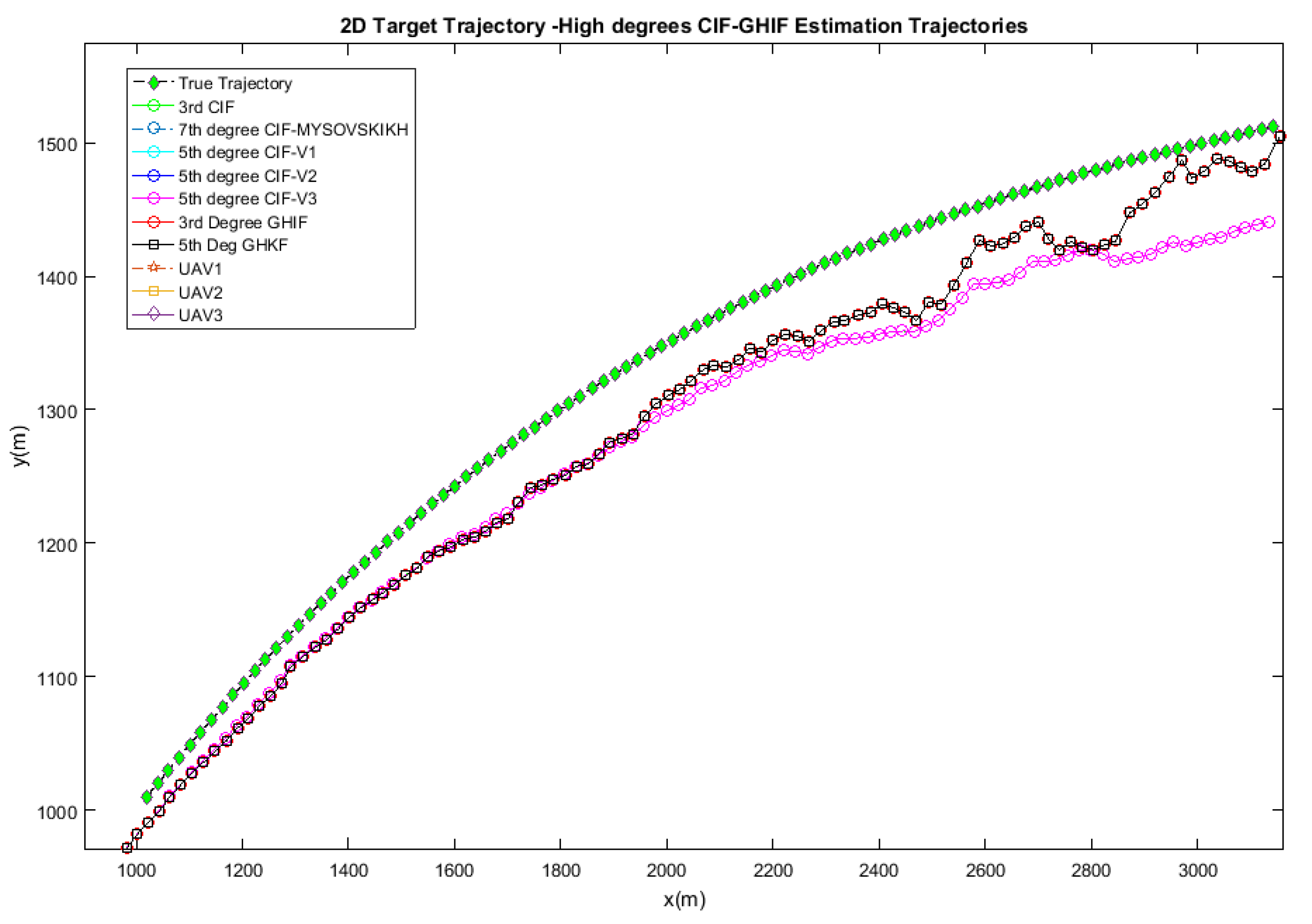
Figure 7.
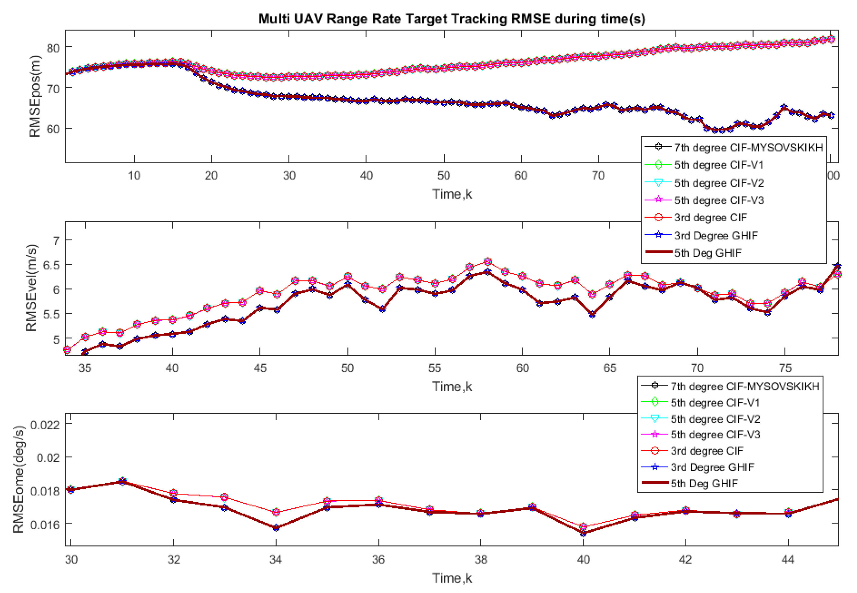
Root mean square error (RMSE) based on range rate Doppler: Results of 7th-degree CIF, 5th-degree CIF, 5th-degree GHIF, 3rd-degree GHIF compared to the true trajectory in green color. The lower error bound was achieved by 7th-degree CIF and 5th-degree GHIF.
Figure 7.
Root mean square error (RMSE) based on range rate Doppler: Results of 7th-degree CIF, 5th-degree CIF, 5th-degree GHIF, 3rd-degree GHIF compared to the true trajectory in green color. The lower error bound was achieved by 7th-degree CIF and 5th-degree GHIF.

Figure 8.
Zoom on range rate Doppler-based trajectory: Results of 7th-degree CIF, 5th-degree CIF, 5th-degree GHIF, 3rd-degree GHIF compared to the true trajectory in green color. The lower error bound was achieved by 7th-degree CIF and 5th-degree GHIF.
Figure 8.
Zoom on range rate Doppler-based trajectory: Results of 7th-degree CIF, 5th-degree CIF, 5th-degree GHIF, 3rd-degree GHIF compared to the true trajectory in green color. The lower error bound was achieved by 7th-degree CIF and 5th-degree GHIF.
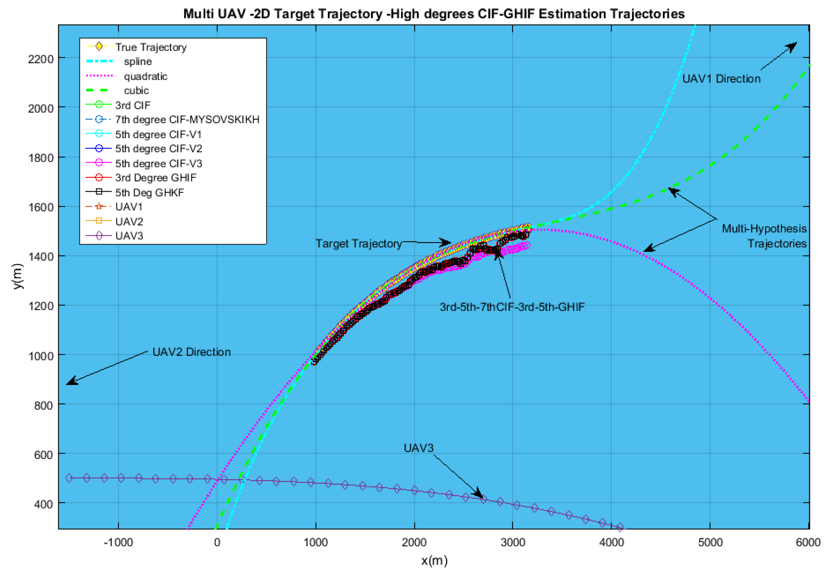
Figure 9.
Range-only Doppler-based estimation: Results of 7th-degree–5th-degree/5th-degree–3rd-degree GHIF trajectory.
Figure 9.
Range-only Doppler-based estimation: Results of 7th-degree–5th-degree/5th-degree–3rd-degree GHIF trajectory.
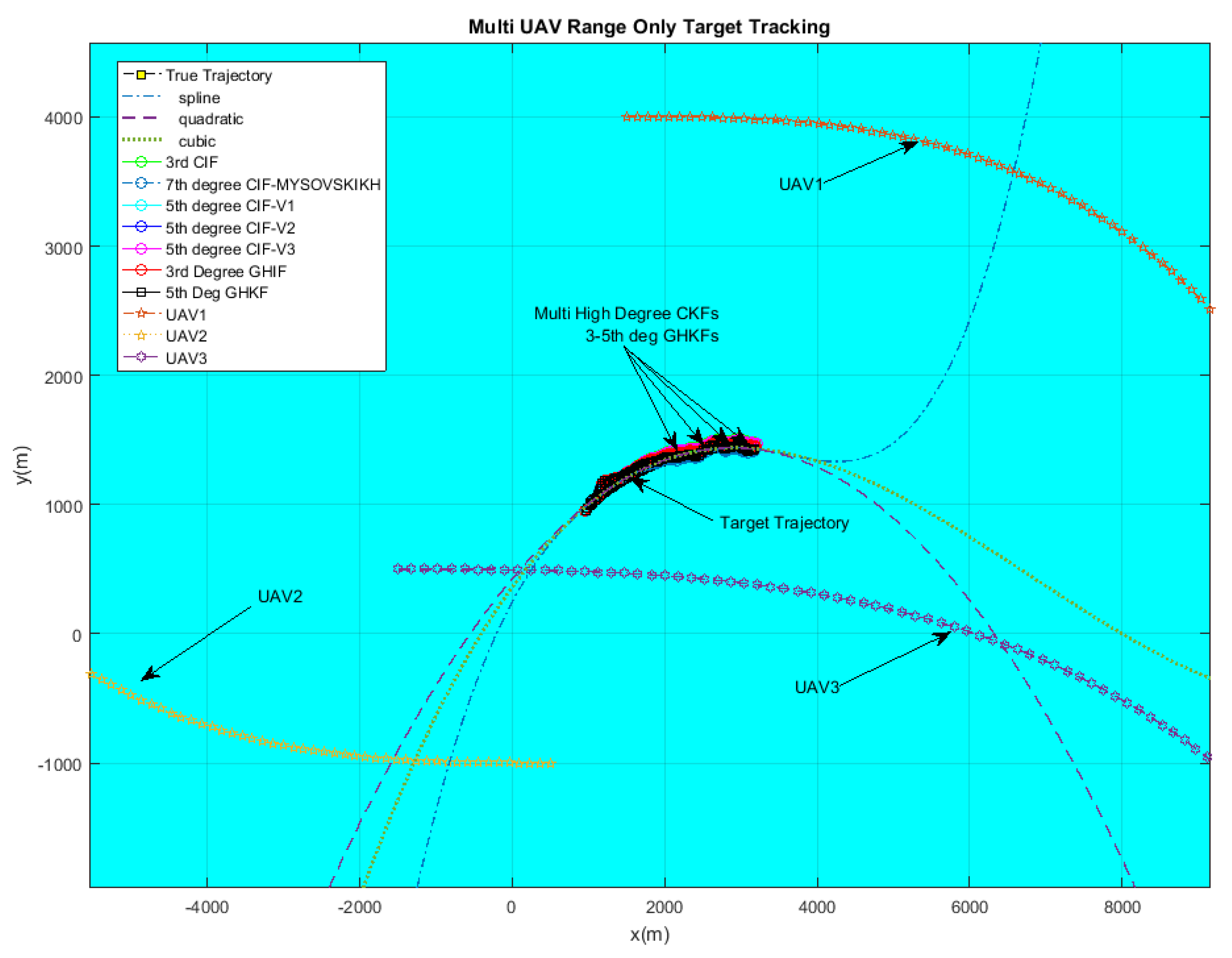
Figure 10.
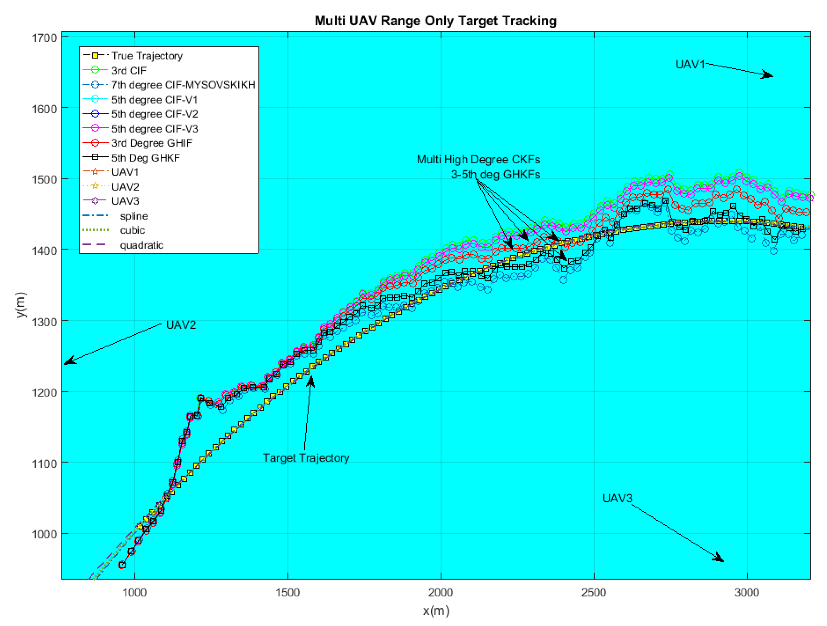
Zoom on range-only Doppler-based estimation: Results of 7th-degree CIF, 5th-degree CIF, 5th-degree GHIF, 3rd-degree GHIF compared to the true trajectory in discontinuous black color.
Figure 10.
Zoom on range-only Doppler-based estimation: Results of 7th-degree CIF, 5th-degree CIF, 5th-degree GHIF, 3rd-degree GHIF compared to the true trajectory in discontinuous black color.

Figure 11.
RMSE of range-only Doppler-based estimation: Results of 7th-degree CIF, 5th-degree CIF, 5th-degree GHIF, 3rd-degree GHIF.
Figure 11.
RMSE of range-only Doppler-based estimation: Results of 7th-degree CIF, 5th-degree CIF, 5th-degree GHIF, 3rd-degree GHIF.

Figure 12.
Larger view of range-only Doppler-based estimation: Results of 7th-degree CIF, 5th-degree CIF, 5th-degree GHIF, 3rd-degree GHIF compared to multiple reference trajectories (spline, quadratic, cubic).
Figure 12.
Larger view of range-only Doppler-based estimation: Results of 7th-degree CIF, 5th-degree CIF, 5th-degree GHIF, 3rd-degree GHIF compared to multiple reference trajectories (spline, quadratic, cubic).


Table 1.
Comparative quadrature points for different rules used in this paper. GHKF: Gauss–Hermite Kalman filter and CKFs: Cubature Kalman filters (3rd-degree, multiple versions of 5rd-degree, Version 1—V1, Version 2—V2, Version 3—V3, Version 4—V4 and 7rd-degree).
Table 1.
Comparative quadrature points for different rules used in this paper. GHKF: Gauss–Hermite Kalman filter and CKFs: Cubature Kalman filters (3rd-degree, multiple versions of 5rd-degree, Version 1—V1, Version 2—V2, Version 3—V3, Version 4—V4 and 7rd-degree).
| Quadrature Rule | Quadrature Points Number |
|---|---|
| 3-point GHKF | |
| 5-point GHKF | |
| 3rd-degree CKF | |
| 5th-degree CKF-V1 | |
| 5th-degree CKF-V2 | |
| 5th-degree CKF-V3 | |
| 5th-degree CKF-V4 | |
| 7th-degree CKF |
Table 2.
Execution time per iteration for different quadrature rules used in this paper.
| Quadrature Rule | Quadrature Points Number | Execution Time (ms) |
|---|---|---|
| 3-point GHKF | 243 | 16.1 |
| 5-point GHKF | 3125 | 206.0 |
| 3rd-degree CKF | 10 | 0.8 |
| 5th-degree CKF-V1 | 43 | 2.2 |
| 5th-degree CKF-V2 | 51 | 1.8 |
| 5th-degree CKF-V3 | 51 | 1.6 |
| 5th-degree CKF-V4 | 32 | 1.4 |
| 7th-degree CKF | 284 | 9.2 |
© 2018 by the authors. Licensee MDPI, Basel, Switzerland. This article is an open access article distributed under the terms and conditions of the Creative Commons Attribution (CC BY) license (http://creativecommons.org/licenses/by/4.0/).
Share and Cite
MDPI and ACS Style
Benzerrouk, H.; Nebylov, A.; Li, M. Multi-UAV Doppler Information Fusion for Target Tracking Based on Distributed High Degrees Information Filters. Aerospace 2018, 5, 28. https://doi.org/10.3390/aerospace5010028
AMA Style
Benzerrouk H, Nebylov A, Li M. Multi-UAV Doppler Information Fusion for Target Tracking Based on Distributed High Degrees Information Filters. Aerospace. 2018; 5(1):28. https://doi.org/10.3390/aerospace5010028
Chicago/Turabian StyleBenzerrouk, Hamza, Alexander Nebylov, and Meng Li. 2018. "Multi-UAV Doppler Information Fusion for Target Tracking Based on Distributed High Degrees Information Filters" Aerospace 5, no. 1: 28. https://doi.org/10.3390/aerospace5010028
Note that from the first issue of 2016, this journal uses article numbers instead of page numbers. See further details here.