Volatility Spillover Effects of the US, European and Chinese Financial Markets in the Context of the Russia–Ukraine Conflict

Abstract

The present study aims to investigate the volatility spillover effects in the international financial markets before and during the Russia–Ukraine conflict. The subject of this paper is the study of the influence of the recent war between Russia and Ukraine on the transmission of volatility between the American, European and Chinese stock markets using the DY methodology. The sample period for daily data is from 1 June 2019 to 1 June 2022, excluding holidays. The volatility spillover index increased during the war period, but this increase remains insignificant compared to that recorded during the COVID-19 pandemic crisis. According to the empirical results, we also found varying levels of dependence and spillover effects between the European, American and Chinese stock indices before and during the Russia–Ukraine conflict.

1. Introduction

The Russia–Ukraine conflict is considered the most serious event in Europe since World War II because it comes at a critical time for the global economy. It has dashed the prospects for global economic recovery from the ravages of COVID-19, at least for now. Since the World Health Organization (WHO) declared the COVID-19 outbreak a public health emergency of international concern, the global economy has been strained by falling financial markets. The conflict between Russia and Ukraine had a significant impact on financial market volatility. Economic sanctions and inflation are the main ways in which the Russia–Ukraine war has impacted global financial markets.

Russia and Ukraine are ranked among the major exporters of various commodities and food products. The conflict between Russia and Ukraine has impacted Russian exports, which are limited due to sanctions; for Ukraine, ports are closed due to the conflict. Wheat futures on the Chicago futures market have already reached 14-year highs due to the disagreement (Josephs 2022). Russian oil and gas are used to heat homes, fuel businesses and fill gas tanks in many European countries. Within days, the conflict fueled global inflation by driving up the price of oil, natural gas and other commodities (Cohen 2022). The conflict between Russia and Ukraine exacerbated existing supply chain problems by threatening to destroy some transportation infrastructure (including ports in Ukraine) and prompting financial sanctions on Russian exports. Due to Turkey’s decision to restrict transit through the Bosphorus and Ukraine’s decision to close commercial shipping, sea freight routes through the Black Sea will be restricted for an unknown period of time. Grain shipments through Russian, Ukrainian and possibly Romanian and Bulgarian ports will be directly affected. During the coronavirus pandemic, this restriction will have ramifications around the world, including in China, which depends on land routes through Russia (en route to Europe). Prior to the pandemic, air transport accounted for 35% of global freight. The EU’s decision to block Russian aircraft and cargo from its airspace will significantly impede air traffic between Russia and Europe and between Europe and Asia. This conflict will also impact land trade routes, as transit through Russia will become extremely difficult (if not impossible from a reputational, compliance or security perspective). These debates have demonstrated the importance of studying volatility spillover effects between international financial markets.

Yazbeck et al. (2022) studied a representative sample of Lebanese household members aged 18 and older (N = 914) to determine the prevalence and correlates of food insecurity, low dietary diversity (DD), unhealthy eating habits and changes in household dietary patterns in response to the Russia–Ukraine war. Binary logistic regression results also revealed that food insecurity was twice as prevalent in households with low monthly income, 35% more prevalent in women and three times more prevalent in participants who were married. They quantified these findings. In order to identify the problems and create solutions to lessen the negative consequences of the war, a systematic approach and an international effort are needed to address how the Russia–Ukraine conflict is affecting food security in Lebanon.

Marfatia (2017) took a new approach to global volatility propagation across 22 of the major stock markets by combining the best aspects of parametric and nonparametric techniques. The strategy of his research work is to examine risk covariation at the national and regional levels by combining wavelet techniques with time-varying conditional volatility. The evidence implies that, in the long run, risk covariation between the U.S. and European markets is strongest, especially at lower frequencies. The integration of a country’s stock market risks is more closely related to the region to which the country belongs at higher (short-term) frequencies and less to the U.S. or other international markets. His research offers new insights showing that risk spillover was mainly limited to lower frequencies. This study differs from our work in that our sample consists of only three global stock market indices while the cited study applies to 22 stock market indices.

This article examines the influence of conflict on the transmission of volatility between the world’s major financial markets, focusing on the American, European and Chinese stock markets. The goal is to use the methodologies proposed by Diebold and Yilmaz (2012, 2014) to investigate the influence of Russia’s uranium war on the transmission of volatility across global financial markets. We will see how foreign currency shocks from a global financial market affect the volatility of a market index’s return.

We can identify the risk of financial contagion of major stock indices on a worldwide level thanks to the effects of volatility spillover. The interconnectedness of the three financial markets inspired this study, which allows us to categorize stock market indices based on the amount of their contribution to contagion effects of volatility before and during the war. We also calculate a worldwide spillover index to determine the overall impact of this conflict on the transmission of volatility in financial markets.

We will show how events related to the Russia–Ukraine conflict have influenced the risk of financial contagion using daily data from 1 January 2019 through 1 June 2022. The period we have chosen in our analysis is characterized by a high volatility of the various international stock market indices due to the evolution of the conflict between these two countries after a partial recovery that characterized the international financial markets that reported significant shocks during the pandemic crisis, which will allow us to analyze the impact of the war on global financial markets.

2. Literature Review

During the last few years, research on financial markets has progressed in the modeling of financial contagion. Several economic studies on the transmission of volatility between financial markets, particularly after the global financial crisis of 2008, have used the term “financial contagion”.

Diebold and Yilmaz (2009) proposed the contagion index (DY’s index), which uses a VAR of order p with N variables and an H-period forecast to assess the interdependence of returns and volatility. On a large number of returns, this index adds the contribution of each variable to the variance of the prediction error of other variables. Yilmaz (2010) investigated the spread of volatility on Asian stock exchanges and discovered that there is a propagation dynamic in the behavior of the indices of spread of returns and spread of volatility in Asia over time.

Diebold and Yilmaz (2012) used generalized vector autoregression (VAR), which generates invariant estimations of the order of the VAR, to calculate volatility deferrals on the American markets for stocks, bonds, currencies and commodities. They demonstrated enormous changes in market volatilities, as well as spillovers of volatility to other markets, during the global financial crisis that began in 2007, while market volatilities were relatively limited before the crisis.

Beraich et al. (2021) studied the impact of the COVID-19 pandemic crisis on the volatility of the Moroccan financial market by applying GARCH models and noticed that the volatility of the MASI stock index increased during the crisis period.

Before and after the 2008 global financial crisis (GFC), Belcaid and El Ghini (2019) assessed the return and volatility spillovers between the stock markets of Morocco, the United States, the United Kingdom, France and Germany as represented by the MASI, S&P 500, FTSE 100, CAC 40 and DAX 30 indices, respectively. Using Diebold and Yilmaz’s methodology, their findings demonstrate a varying degree of financial interconnectedness between the stock markets in Morocco and the aforementioned developed nations. Additionally, they discovered a substantial rise in the spillover index during the immediate aftermath of the financial crisis, demonstrating that the U.S. and European stock markets were the most negatively impacted.

To create a volatility index, Beraich and El Main (2022) used the DY approach in conjunction with the daily stock prices of Moroccan financial organizations. Their empirical findings show that the COVID-19 issue caused the volatility spillover index to grow. Additionally, they discovered various levels of pre- and post-COVID-19 pandemic crisis interconnectedness and spillover effects between the six publicly traded Moroccan banks and the Moroccan banking sector stock index.

Li et al. (2022) used input–output analysis and complex network methodologies to examine a path analysis of the influence of the Russian–Ukrainian conflict on the world from a regional, industrial and critical path perspective. In four points, they outlined their findings: (1) Due to the fact that domestic industry interaction tends to determine how Russia’s economy develops, sanctions may not have much of an impact on the country. (2) Germany, the United States, France and South Korea are all heavily interdependent economically, as are Russia and China. (3) Industries that serve as resource processing hubs, significant suppliers or consumers for adjacent industries, or that have low symmetry and high clustering, such as mining and quarrying, power generation, coke and refined petroleum products, chemicals and chemical products and construction in Russia, must be examined in particular. (4) Important roles are played by key industries in Russia as providers of Chinese coke and refined petroleum products as well as the Japanese construction sector, as well as consumers of German machinery and equipment and professional, scientific and technological activities from the United States.

The crisis between Russia and Ukraine has had repercussions around the world. Major commodity markets (oil, gas, platinum, gold and silver) have seen significant changes in supply and prices. The prolonged violence has had a significant impact on commodity prices and financial markets around the world. Since the beginning of the financial crisis in 2008, which directly affected the oil and gold markets, this effect can be considered the biggest change. Alam et al. (2022) conducted a study to show how the Russian invasion affected the dynamic interconnectedness of five commodities, the G7 and BRIC (leading stock) markets. They used the time-varying parameter vector autoregression (TVP-VAR) technique, which captures how spillovers are formed by distinct crisis periods, and found that all commodities and markets are highly interconnected (G7 and BRIC). Their results show that during this invasion crisis, the stock markets of the US, Canada, China and Brazil, as well as gold and silver (commodities), are the receivers of shocks from other commodities and markets.

3. Data

The following stock market indices were chosen to analyze the impact of the Russia–Ukraine conflict on volatility spillover effects on international financial markets:

• Dow Jones Europe (Europe);
• MSCI-USA (United States);
• MSCI China (China).

Our database runs from 1 January 2019 to 1 June 2022. To meet the objectives of the study, we used a cut-off date (24 February 2022) to split the data into two sub-periods: before and during the Russia–Ukraine conflict.

3.1. Methodology

The evaluation and analysis of volatility spillovers between the main international markets (US, Europe and China) is the basis of our study. To perform the evaluation and analysis of volatility spillovers between the main international markets, we examined the key strategies of Diebold and Yilmaz (2012, 2014).

The return and volatility of a stock market index over time evolve under internal shocks (asset-specific shocks) or external shocks from other stock market indices. The objective is to determine how much of the overall expected volatility for each index is contributed by the two different types of shocks.

In our study, we use a technique created by Diebold and Yilmaz (2012, 2014). Generalized vector autoregression (VAR) models of order p are used as the basis for this approach. This method has the advantage of producing generalized, order-invariant, variance decompositions that allow for correlated shocks but appropriately compensate for correlation rather than orthogonalizing shocks.

3.1.1. VAR (p) Model

A p-order multivariate vector autoregressive stochastic process, $VAR\left(p\right)$, is a generalization of the univariate autoregressive stochastic process$AR\left(p\right)$. N is the total number of variables under investigation, and 1 is the dimension of the $VAR\left(p\right)$ process. Each variable’s time course is represented by an equation that functions as a function of the variable’s time-lagged values, the lagged values of the other variables in the model, and an error term.

Each financial variable in a $VAR\left(p\right)$ model is represented as a linear combination of its historical values and the historical values of the other financial variables in the system. We represented these variables as a system of linear equations where the number of equations corresponds to the number of financial variables because we have a database of many time series that influence one another.

If not, we will have a system of N linear equations for N time series that affect each other.

A model $VAR\left(p\right)$ for N processes $\left({(X_{1,t})}_{tϵ𝕫},{(X_{2,t})}_{tϵ𝕫}\dots \dots \dots .. {(X_{N,t})}_{tϵ𝕫}\right)$ is presented as a system of N linear equations as follows:

$$\{\begin{array}{c}{X}_{1,t}=c_1+\left[{\mathsf{\Phi }}_{11,1}{X}_{1,t-1}+{\mathsf{\Phi }}_{12,1}{X}_{2,t-1}+\dots +{\mathsf{\Phi }}_{1N,1}{X}_{N,t-1}\right]+\dots +\left[{\mathsf{\Phi }}_{11,p}{X}_{1,t-p}+{\mathsf{\Phi }}_{12,p}{X}_{2,t-p}+\dots +{\mathsf{\Phi }}_{1N,p}{X}_{N,t-p}\right]+{\epsilon }_{1,t}\\ X_{2,t}=c_2+\left[{\mathsf{\Phi }}_{21,1}{X}_{1,t-1}+{\mathsf{\Phi }}_{22,1}{X}_{2,t-1}+\dots +{\mathsf{\Phi }}_{2N,1}{X}_{N,t-1}\right]+\dots +\left[{\mathsf{\Phi }}_{21,p}{X}_{1,t-p}+{\mathsf{\Phi }}_{22,p}{X}_{2,t-p}+\dots +{\mathsf{\Phi }}_{2N,p}{X}_{N,t-p}\right]+{\epsilon }_{2,t}\\ .\\ .\\ .\\ X_{N,t}=c_N+\left[{\mathsf{\Phi }}_{N1,1}{X}_{1,t-1}+{\mathsf{\Phi }}_{N2,1}{X}_{2,t-1}+\dots +{\mathsf{\Phi }}_{NN,1}{X}_{N,t-1}\right]+\dots +\left[{\mathsf{\Phi }}_{N1,p}{X}_{1,t-p}+{\mathsf{\Phi }}_{N2,p}{X}_{2,t-p}+\dots +{\mathsf{\Phi }}_{NN,p}{X}_{N,t-p}\right]+{\epsilon }_{N,t}\end{array}$$

(1)

A generalized $VAR\left(p\right)$ model can be presented in matrix form as follows:

$$X_t=C+{\displaystyle \sum }_{\mathrm{k}=1}^{\mathrm{p}}{\mathrm{A}}_{\mathrm{k}}{X}_{t-k}+{\epsilon }_t=C+{\mathrm{A}}_1{X}_{t-1}+{\mathrm{A}}_2{X}_{t-2}+\dots +{\mathrm{A}}_p{X}_{t-p}+{\epsilon }_t$$

(2)

$$\left(\begin{array}{c}{X}_{1,t}\\ X_{2,t}\\ ⋮\\ X_{N,t}\end{array}\right)=\left(\begin{array}{c}{c}_1\\ c_2\\ ⋮\\ c_N\end{array}\right)+\left[\left(\begin{array}{cccc}{\mathsf{\Phi }}_{11,1}& {\mathsf{\Phi }}_{12,1}& \cdots & {\mathsf{\Phi }}_{1N,1}\\ {\mathsf{\Phi }}_{21,1}& {\mathsf{\Phi }}_{22,1}& \cdots & {\mathsf{\Phi }}_{2N,1}\\ ⋮& ⋮& \ddots & ⋮\\ {\mathsf{\Phi }}_{N1,1}& {\mathsf{\Phi }}_{N2,1}& \cdots & {\mathsf{\Phi }}_{NN,1}\end{array}\right)\left(\begin{array}{c}\begin{array}{c}{X}_{1,t-1}\\ X_{2,t-1}\\ ⋮\end{array}\\ X_{N,t-1}\end{array}\right)+\cdots +\left(\begin{array}{cccc}{\mathsf{\Phi }}_{11,p}& {\mathsf{\Phi }}_{12,p}& \cdots & {\mathsf{\Phi }}_{1N,p}\\ {\mathsf{\Phi }}_{21,p}& {\mathsf{\Phi }}_{22,p}& \cdots & {\mathsf{\Phi }}_{2N,p}\\ ⋮& ⋮& \ddots & ⋮\\ {\mathsf{\Phi }}_{N1,p}& {\mathsf{\Phi }}_{N2,p}& \cdots & {\mathsf{\Phi }}_{NN,p}\end{array}\right)\left(\begin{array}{c}\begin{array}{c}{X}_{1,t-p}\\ X_{2,t-p}\\ ⋮\end{array}\\ X_{N,t-p}\end{array}\right)\right]+\left(\begin{array}{c}{\epsilon }_{1,t}\\ {\epsilon }_{2,t}\\ ⋮\\ {\epsilon }_{N,t}\end{array}\right)$$

(3)

where

• $C—\mathrm{vector} \left(N\times 1\right) \mathrm{of} \mathrm{the} N \mathrm{constants} c_i \mathrm{of} \mathrm{the} \mathrm{equations} \mathrm{of} \mathrm{the} VAR\left(p\right) \mathrm{model}$;
• $X_t—\mathrm{vector} \left(N\times 1\right) \mathrm{of} \mathrm{the} N \mathrm{variables} X_{i,t} \mathrm{of} \mathrm{the} VAR\left(p\right) \mathrm{model}$;
• ${\epsilon }_t—\mathrm{vector} \left(N\times 1\right) \mathrm{of} \mathrm{the} N \mathrm{innovations} \mathrm{of} \mathrm{the} VAR\left(p\right) \mathrm{model}$;
• ${\mathrm{A}}_{k }—\mathrm{matrix} \left(N\times N\right) \mathrm{of} \mathrm{the} \mathrm{coefficients} \mathrm{of} \mathrm{the} VAR\left(p\right) \mathrm{model}$;
• $X_{t-k}—\mathrm{vector} \left(N\times 1\right) \mathrm{of} \mathrm{the} \mathrm{N} \mathrm{variables} X_{i,t} \mathrm{lagged} \mathrm{at} \mathrm{order} k.$

3.1.2. Volatility of Returns

There are many measures of return of a stock index; a frequently used one is the geometric return or the log return, which involves calculating the logarithm of the differential of the values in t and t − 1.

The return of this stock at time t is defined as follows:

$$R_t=\mathit{log}\left(\frac{P_t}{P_{t-1}}\right)=\mathit{log}\left(P_t\right)-\mathit{log}\left(P_{t-1}\right)=\mathit{log}\left(r_t+1\right) \mathrm{where} t=1, 2, \dots , n$$

(4)

and

$$r_t=\frac{P_t-P_{t-1}}{P_{t-1}}$$

(5)

where

• $R_t—$the log return of a stock at time t;
• $r_t—$the algebraic return of a stock at time t;
• $P_t—$the stock price at time t.

When assessing our financial series, we frequently take into account daily log returns. In the financial literature, there are various techniques for estimating asset volatility. Garman and Klass (1980) estimated the volatility of financial series using current information based on past daily prices (opening, closing, high and low prices). These models employ historical data on stock prices for the renowned GARCH family (Engle and Kroner 1995; Engle and Sheppard 2001; Engle 2002; Francq and Zakoïan 2010). The approach proposed in this paper is that of Parkinson (1980), which gives an estimate of the variance of returns based on the highest prices $(H_i)$ and the lowest prices $(L_i)$.

The Parkinson volatility is then obtained using the following formula:

$${\tilde{\sigma }}_{it}^2=0.361\times {(\ln \left(H_{it}\right)-\ln \left(L_{it}\right))}^2$$

(6)

3.1.3. Decomposition of the Variance of the Forecast Error (FEVD)

Given a $VAR\left(p\right)$ model with N variables, the decomposition of the variance of the forecast error of the variable $X_{i,t}$ determines the percentage of the variance of this error that is explained by a shock to another variable $X_{j,t}$. The variance of the forecast error of i represents 100%, and each variable j of the system of its $\mathit{VAR}\left(p\right)$ model will make a contribution to explain this variance.

The forecast error variance decomposition (FEVD) is used to indicate how much information each variable contributes to the other variables in the $\mathit{VAR}\left(p\right)$ model. It finds out how much the forecast error variance of each variable can be explained by shocks to the other variables that come from the outside.

Diebold and Yilmaz (2012) calculate the forecast error variance decompositions as follows:

$$d_{ij}^{\mathrm{H}}=\frac{{\mathsf{\sigma }}_{jj}^{-1}{\mathsf{\Sigma }}_{h=0}^{\mathrm{H}-1} {\left({\mathrm{e}}_i^{\prime }{\mathrm{A}}_h{\mathsf{\Sigma }\mathrm{e}}_j\right)}^2}{{\mathsf{\Sigma }}_{h=0}^{\mathrm{H}-1}({\mathrm{e}}_i^{\prime }{\mathrm{A}}_h{\mathsf{\Sigma }\mathrm{A}}_h^{\prime }{\mathrm{e}}_i)}$$

(7)

where

• $d_{ij}^{\mathrm{H}}$—explains the shocks contributed by the financial variable $X_j$ to the variance of the forecast error of another variable$X_i$;
• ${\sigma }_{jj}$—standard deviation of the residual for the $j$th equation in the model;
• $e_i$—selection vector, with 1 for the $i$th element and 0 otherwise;
• $\mathsf{\Sigma }$—vector of variances of the $\epsilon$ disturbances.

The individual row sum of $d_{ij}\left(\mathrm{H}\right)$ is not equal to unity $\left({\mathsf{\Sigma }}_{j=1}^{\mathrm{N}}{d}_{ij}^{\mathrm{g}}\ne 1\right)$. Therefore, the row sum result is used to divide the individual component of the decomposition matrix to normalize it. This is expressed by the following calculation:

$${\widetilde{ d}}_{ij}^H=\frac{d_{ij}^{\mathrm{H}}}{{\mathsf{\Sigma }}_{j=1}^{\mathrm{N}}{d}_{ij}^{\mathrm{H}}}$$

(8)

where

• $d_{ij}^{\mathrm{H}}$—the proportion of shocks contributed by the financial variable $X_j$ to the variance of the forecast error of another variable$X_i$; ${\mathsf{\Sigma }}_{j=1}^{\mathrm{N}}{\widetilde{d }}_{ij}^{\mathrm{H}}=1$.

3.1.4. Spillover Index

The total spillover index determines the contribution of volatility shocks of all variables to the total variance of forecast errors:

$$S^{\mathrm{H}}=\frac{{\mathsf{\Sigma }}_{i,j=1,i\ne j}^{\mathrm{N}}{\tilde{d}}_{ij}^{\mathrm{H}}}{{\mathsf{\Sigma }}_{i,j=1}^{\mathrm{N}}{\tilde{d}}_{ij}^{\mathrm{H}}}\times 100=\frac{{\mathsf{\Sigma }}_{i,j=1,i\ne j}^{\mathrm{N}}{\tilde{d}}_{ij}^{\mathrm{H}}}{\mathrm{N}}\times 100 \mathrm{with} i\ne j$$

(9)

The directional spillovers received by institution i from all other institutions j (from others) are

$$S_{i \overleftarrow{\mathit{f}\mathit{r}\mathit{o}\mathit{m}} j}^{\mathrm{H}}=\frac{{\mathsf{\Sigma }}_{i,j=1,i\ne j}^{\mathrm{N}}{\tilde{d}}_{ij}^{\mathrm{H}}}{{\mathsf{\Sigma }}_{j=1}^{\mathrm{N}}{\tilde{d}}_{ij}^{\mathrm{H}}}\times 100$$

(10)

The directional spillovers transmitted by institution i to all other institutions j (to others) are

$$S_{i \overrightarrow{\mathit{t}\mathit{o}} j}^{\mathrm{H}}=\frac{{\mathsf{\Sigma }}_{j=1,i\ne j}^{\mathrm{N}}{\tilde{d}}_{ij}^{\mathrm{H}}}{{\mathsf{\Sigma }}_{j=1}^{\mathrm{N}}{\tilde{d}}_{ij}^{\mathrm{H}}}\times 100$$

(11)

The difference between the gross shocks sent from asset i and the gross shocks received from all other assets can be used to determine the net spillovers from asset i to all other assets:

$$NS=S_{i \overrightarrow{\mathit{t}\mathit{o}} j}^{\mathrm{H}}-S_{i \overleftarrow{\mathit{f}\mathit{r}\mathit{o}\mathit{m}} j}^{\mathrm{H} }$$

(12)

The Diebold–Yilmaz variance decomposition table, which is displayed below in

Table 1. Variance decomposition of Diebold and Yilmaz.

	${\mathbf{X}}_1$	${\mathbf{X}}_2$	$\dots$	${\mathbf{X}}_{\mathit{N}}$	Contribution from Others
${\mathrm{X}}_1$	$d_{11}\left(\mathrm{H}\right)$	$d_{12}\left(\mathrm{H}\right)$	$\dots$	$d_{1N}\left(\mathrm{H}\right)$	${\mathsf{\Sigma }}_{j=1}^{\mathrm{N}}{d}_{1j}\left(\mathrm{H}\right)j\ne 1$
${\mathrm{X}}_2$	$d_{21}\left(\mathrm{H}\right)$	$d_{22}\left(\mathrm{H}\right)$	$\dots$	$d_{2N}\left(\mathrm{H}\right)$	${\mathsf{\Sigma }}_{j=1}^{\mathrm{N}}{d}_{1j}\left(\mathrm{H}\right)j\ne 2$
$⋮$	$⋮$	$⋮$	$\ddots$	$⋮$	$⋮$
${\mathrm{X}}_N$	$d_{N1}\left(\mathrm{H}\right)$	$d_{N2}\left(\mathrm{H}\right)$	$\dots$	$d_{NN}\left(\mathrm{H}\right)$	${\mathsf{\Sigma }}_{j=1}^{\mathrm{N}}{d}_{Nj}\left(\mathrm{H}\right)j\ne \mathrm{N}$
Contribution to Others	${\mathsf{\Sigma }}_{i=1}^{\mathrm{N}}{d}_{i1}\left(\mathrm{H}\right)$ $i\ne 1$	${\mathsf{\Sigma }}_{i=1}^{\mathrm{N}}{d}_{i2}\left(\mathrm{H}\right)$ $i\ne 2$	$\dots$	${\mathsf{\Sigma }}_{i=1}^{\mathrm{N}}{d}_{i3}\left(\mathrm{H}\right)$ $i\ne 3$	$\frac{1}{\mathrm{N}}{\mathsf{\Sigma }}_{i,j=1}^{\mathrm{N}}{d}_{ij}\left(\mathrm{H}\right)i\ne j$

, contains the underlying variance decomposition based on a daily VAR that was located using the generalized variance decomposition. The estimated variance of the H-day forecast error of index i due to shocks from index j is also included in the $i{j}^{th}$ entry. The assets in the first row are where the spillovers originate. The assets that receive spillovers are listed in the first column. The “Contribution from Others” column of the asset indicated in the first column displays the total of its spillovers. The spillovers from the asset indicated in the first row are added up in the row labeled “Contribution to Others”.

The difference in total directional spillovers is shown in the “Spillover Net” row (“Contribution to Others” minus “Contribution from Others”). The sum of all non-diagonal columns and rows divided by the sum of all diagonal columns and rows, stated as a percentage, is known as the total spillover index.

The benefit of utilizing this approach is that it dynamically models the overflow while taking into account temporal variations.

4. Preliminary Analysis

By analyzing the evolution of the values of the stock market indices of China, United States and Europe before and during the period of the war crisis presented in Figure 1, we noticed that these stock prices were affected by the effects of the Russia–Ukraine conflict. We noted that these graphs are characterized by a downward trend during the first months of 2022 (period of the war crisis in Ukraine). Figure 2 displays the evolution of the daily returns of the three indices.

The log returns of the indices in the two specified sub-periods are summarized in

Table 2. Descriptive statistics and stationarity results (before the war crisis).

Before the War Crisis	MSCI-CHINA	MSCI-USA	MSCI-EUROPE
Mean	0.0038	0.0030	−0.0023
Median	0.0042	0.0019	0.0013
Maximum	0.0284	0.0345	0.0299
Minimum	−0.0224	−0.0241	−0.0166
Std. Dev.	0.0119	0.0093	0.0082
Skewness	−0.2214	0.2733	0.8145
Kurtosis	4.8881	6.3578	6.3578
Normality test: Jarque–Bera Probability	10.3304	18.3255	11.2944
	0.0085	0.0001	0.0035
Unit root test: ADF Probability	−24.2271	−23.1485	−25.4371
	0	0	0

and

Table 3. Descriptive statistics and stationarity results (during the war crisis).

During the War Crisis	MSCI-CHINA	MSCI-USA	MSCI-EUROPE
Mean	−0.0016	−0.0016	−0.0012
Median	−0.0013	−0.0010	−0.0015
Maximum	0.1454	0.0298	0.0621
Minimum	−0.0765	−0.0901	−0.0506
Std. Dev.	0.0302	0.0199	0.01802
Skewness	1.5035	−1.3067	0.3401
Kurtosis	9.8526	6.8789	5.2154
Normality test: Jarque–Bera Probability	165.6701	64.7179	15.8884
	0	0	0.0003
Unit root test: ADF Probability	−17.7735	−15.2305	−19.0789
	0	0	0

using certain descriptive statistics (before and during war). For all series, the kurtosis is significantly higher than 3, indicating a severe return distribution (leptokurtic). Additionally, the data show a statistically significant departure from the Gaussian distribution according to the Jarque–Bera normalcy test (p < 0.0001). The log return series has autocorrelation, according to the statistics from the Ljung–Box (1978) test.

The log returns of the three series were subjected to the common augmented Dickey–Fuller (ADF) unit root test, as shown in Table 2 and Table 3. At the 1% significance level, the ADF statistic falls short of its crucial values. As a result, these series can be used for additional analysis because they lack unit roots and are not moving.

5. Empirical Results

In this section, we measure the volatility spillovers of returns during the pre-crisis and during-crisis sub-periods for the assets of the three stock market indices. The spillover index will allow us to indicate the connectivity and volatility transmission between each index pair $\left(i,j\right)$ in both directions ($i\overrightarrow{ to }j and i \overleftarrow{from} j \left(\forall i\ne j\right)$) and between each index $i$ and all other indices ($i\overrightarrow{ to all }j and i \overleftarrow{from all} j \left(\forall i\ne j\right)$).

Here, we present the description of the static spillover index for returns and volatility. In addition, we calculate the average directional spillovers and the average net spillovers before and during the Russian war crisis in Ukraine. This can tell us a lot about how the spillover effect is passed on between the indices that make up the international financial markets.

The KPPS basalized variance decomposition is the variance decomposition that underlies

Table 4. Volatility spillover index (pre-crisis period).

	MSCI-CHINA	MSCI-EUROPE	MSCI-USA	Contribution from Others
MSCI-CHINA	86.82	8.48	4.70	13.18
MSCI-EUROPE	10.40	81.32	8.28	18.68
MSCI-USA	5.66	6.74	87.60	12.40
Contribution to Others	16.06	15.22	12.98	44.26
Contribution to Others Including Own	102.88	96.54	100.58
Spillover Net *	2.88	−3.46	0.58	SI = 14.75% **

* spillover net = contribution to others − contribution from others; ** spillover index.

and

Table 5. Volatility spillover index (during-crisis period).

	MSCI-CHINA	MSCI-EUROPE	MSCI-USA	Contribution from Others
MSCI-CHINA	83.04	10.25	6.72	16.96
MSCI-EUROPE	4.63	73.16	22.21	26.84
MSCI-USA	3.34	1.18	95.48	4.52
Contribution to Others	7.97	11.43	28.93	48.32
Contribution to others Including Own	91.00	84.59	124.41
Spillover Net *	−9.00	−15.41	24.21	SI = 16.11% **

* spillover net = contribution to others − contribution from others; ** spillover index.

. Additionally, the $i{j}^{th}$ entry represents the anticipated variation of index i’s 10-day forecast error as a result of shocks from index j. The assets that cause the spillovers are displayed in the first row. The assets receiving the spillovers are identified in the first column. The total spillovers that the asset indicated in the first column has received are shown in the column labeled “Contribution from Others”. The value in the “Contribution to Others” row for the asset listed in the first row represents the total of spillovers.

The difference in total directional spillovers is shown in the “Spillover Net” row (“Contribution to Others” minus “Contribution from Others”). The sum of all non-diagonal columns and rows expressed as a percentage of the sum of all diagonal columns and rows is known as the total spillover index.

5.1. Pre-Crisis Sub-Period: From 1 January 2019 to 23 February 2022

Table 4 provides an approximate decomposition of the volatility spillover index before the COVID-19 pandemic crisis.

Analyzing the results in Table 4, we notice that the gross directional spillovers of the MSCI-EUROPE index are the strongest; its “contribution from others” value is equal to 18.68% of the variance of the volatility forecast errors, which means that 18.68% of the volatility shocks of the European index are due to the shocks of the stock market indices of China and the United States. Conversely, the European index is responsible for 15.22% of the variance of the volatility forecast errors of the other indices (MSCI-CHINA and MSI-USA). As for the net spillover effects of the European index, they are equal to −3.46%. This negative value shows that the weight of transmitted volatility shocks is lower than the weight of the shocks received for the pre-crisis period.

Individually, the gross directional volatility spillovers from the MSCI-EUROPE index to the other indices are 8.48% for the MSCI-CHINA and 6.74% for the MSCI-USA; this indicates that 8.48% of the volatility shocks of the Chinese index are produced because of the European market shocks, and only 6.74% of the volatility shocks for the U.S. market index are due to the volatility shocks of the Europe index. In general, we notice that in the gross directional spillovers of the European stock market index, the “contribution to others” value remains at 15.22% while the “from others” contribution amounts to 18.68%, which gives a negative net spillover value of −3.46% for this index. We therefore conclude that the volatility spillovers transmitted by this index before the crisis are lower compared to the shocks received. The Chinese market index transmitted 16.06% of these shocks to the other indices while it received only 13.18%, which gives positive net spillovers of 2.88%. The MSCI-USA index has positive net spillovers of 0.58%, this value close to 0 shows that this market is almost neutral because there is not a big difference between the weight of the shocks transmitted and the shocks received from other markets.

The spillover index amounts to 14.75%; this index presents a substantial key figure of the summary results, as it shows that 14.75% of the forecast error variance results from volatility spillovers. Therefore, on average, the spillovers transmitted in the three international stock markets selected in our study are significantly large, and they reflect a real level of financial connectivity between the three stock indices.

5.2. During-Crisis Sub-Period: From 24 February 2022 to 1 June 2022

Table 5 presented above provides an approximate decomposition of the volatility spillover index during the war crisis.

During the war crisis, the gross directional spillovers from each market increased significantly. In fact, Table 5 shows that the U.S. market is responsible for 28.93% of the error in the volatility forecasts of the other two markets during the pandemic crisis—up from 12.98% before the crisis. The value of shocks transmitted from the U.S. market to the Chinese and European markets increased significantly during the war.

The “from others” value of the MSCI-USA index fell from 12.4% (pre-crisis) to 4.52% (during the crisis), indicating that the magnitude of volatility shocks to the U.S. index caused by shocks to the other indices was negatively affected by the war crisis.

As for the net spillover of the U.S. index during the war, it is +24.21%. This positive figure shows that the weight of the volatility shocks that are transmitted is stronger than the shocks that are received during this crisis.

During the crisis, the net spillover of the MSCI-EUROPE index changed from −3.46% to −15.41%, which is a significant change. The spillover from the U.S. and Chinese indices to the European market index during the crisis was much higher than that before the crisis, from 18.68% to 26.84%. The European index, on the other hand, transferred 11.43% to the other indices during the war compared to 15.22% before the war.

Finally, the contribution of volatility shocks “from others” for the MSCI-CHINA index changed from 13.18% to 16.96%, and the MSCI-CHINA “to others” value changed from 16.06% to 7.97%. During the crisis sub-period of the Russia–Ukraine conflict, the net effects of the Chinese market decreased significantly from +2.88% to −9%.

In performing a pairwise static analysis, it is interesting to note that the spillover from the U.S. market shocks received from the European index was apparently the largest and represents the largest contribution (22.21%), Conversely, for the U.S. index, the volatility shocks received by this index from the MSCI-EUROPE index represent the smallest contribution of 1.18%.

The spillover index is larger during the war compared to the pre-war period; it reached almost 16.11%, compared to 14.75% before the crisis. This increase is due to the fact that the effects of the crisis on the assets of the three markets became stronger.

All these changes are due to the fact that the effects of the crisis are spreading more rapidly through the international stock markets.

5.3. Dynamic Spillover Index (before and during War Crisis)

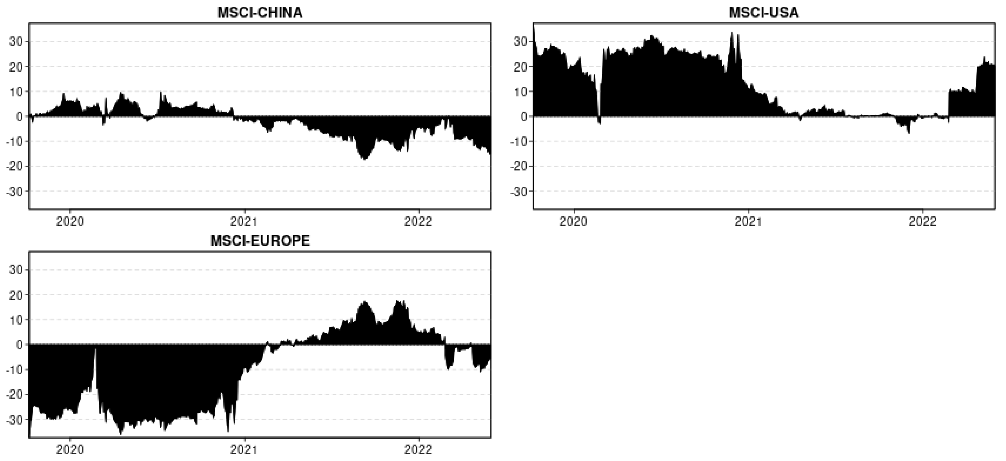
Figure 3 presents the evolution of the conditional volatility of the stocks of the three international stock market indices selected in our study. This remarkable fluctuation in volatility requires a dynamic analysis of the transmission of volatility shocks between the three indices, the red line corresponds to the beginning of the Russian war period in Ukraine.

In the following, we will perform a dynamic analysis of the rolling sample. It is important to note that most studies in this area use rolling samples of 200 days and forecast errors of 10 days, but because of the short duration of the Russian war in Ukraine that started a few months ago, we have plotted the volatility spillover curves using rolling samples of 50 days and forecast errors of 5 days.

5.3.1. Total Volatility Spillover Index

The volatility spillover index in Figure 4 shows a usually dynamic movement and exhibits a minor trend, occasionally increasing and occasionally decreasing, starting from a value slightly above 30% toward the end of 2019. the red line corresponds to the beginning of the Russian war period in Ukraine.

This index presents a dramatic decline in early 2020 after an increase in mid-2020. This increase is followed by a gradual decline at the end of the year 2020. The year 2021 is marked by a small fluctuation of the spillover index around 8%, and during the year 2022, the total spillover index increased once again, reaching values close to 20%.

The high volatility spillover values observed in Figure 4 during 2020 characterize the COVID-19 pandemic and the war crisis and its consequences for the international financial markets.

5.3.2. Total Directional Spillover

We shall show a dynamic analysis of the overall directional connectedness for each index below using sliding estimation windows.

We will concentrate on the directional connection dynamics over time.

For each stock index, Figure 5 and Figure 6 show the total directional connectivity (“to others” for Figure 5 and “from others” for Figure 6). Figure 7 then shows the net total directional connectivity curves. The “to others” and “from others” directional spillover curves do not have the same trend or size, which is the first thing to note in Figure 7 and Figure 8 regarding the “to” and “from” curves. Compared to the “to others” curves, the “from others” curves are significantly smoother. Some of these shocks can be propagated to other indices since stock market indices are susceptible to both external shocks and their own volatility shocks as a result of past shocks. Some of these shocks are minuscule and insignificant, but when an index experiences one, it is probable that the contagion effect it has on other indices will be significantly greater.

In Figure 5, we can see that the “from others” connectivity curves for each index vary across indices during the war period, with the “from others” value being higher for MSCI-EUROPE and MSCI-CHINA and very low for MSCI-USA.

For the “to others” connectivity measures in Figure 6, we notice that the U.S. market transmitted a large amount of volatility shocks to the other markets during the war while the contribution to others for the Chinese index is the lowest. Each index has a different total connectivity to the other indices.

The MSCI-USA index transmits shocks that have a higher weight than the shocks received by the other markets the majority of the time, according to our analysis of the variance of the net spillover of volatility shown in Figure 7. The U.S. index has practically all positive net spillover values. The net spillovers for the other indices are typically more adverse than favorable. Shocks that have a greater weight than the shocks communicated during the war were applied to the MSCI-CHINA and MSCI-EUROPE indices.

5.3.3. Total Directional Spillover Pairwise

When analyzing financial contagion, pairwise volatility connection analysis is crucial. It is worthwhile to emphasize the significance of pairwise connection as a gauge of the transmission of volatility shocks among the three stock market indices. The rolling sample windows show the importance of pairwise connection measurements. It is crucial to look at the volatility relationships between the index pairs since the volatility of one financial institution might influence the volatility of another.

Since there are three indices (USA, CHINA and EUROPE) in our sample, it is therefore necessary to present graphs of volatility connectivity for each of the three pairs in order to analyze how these shocks led to dynamic volatility connectivity between the index pairs during the Russian war in Ukraine.

Analyzing the variation of net volatility spillovers by the pairs shown in Figure 8, we noticed that the MSCI-EUROPE/MSCI-USA pair values are almost all negative, which shows that the European index receives volatility shocks from the MSCI-USA index that are of greater magnitude than those it transmits to the MSCI-USA index. For the MSCI-CHINA/MSCI-USA pair, the degree of connectivity is very low, with small positive or negative values very close to zero. Finally, for the MSCI-CHINA/MSCI-EUROPE pair, the degree of connectedness is positive in 2020 and negative from 2021 onwards, with significant negative values during the war period.

5.3.4. Robustness Assessment of the Total Connectivity

We analyze the reliability of our findings with reference to the selection of the VAR(p) model parameters before wrapping up this section. We have looked into estimation window sizes of 200 days and 10-day forecast horizons. The results are shown in Figure 9, where the blue band corresponds to an interval (from 10% to 90%) based on 100 randomly selected orders, and the black solid line corresponds to our reference order.

The series changes over time with remarkable consistency, which amply demonstrates the dependability of our VAR model estimation findings with respect to the order p of the VAR model or the sliding window’s time horizon in the dynamic analysis.

It should be noted that the range (from 10% to 90%) based on 100 random orders of total connection is extremely narrow.

6. Conclusions

This study presents important results on the connectivity and volatility spillovers between international stock indices in the context of the Russian war in Ukraine that characterized the year 2022. The approach adopted is the one suggested by Diebold and Yilmaz (2012, 2014).

The daily data of the stock market indices of the three markets (American, European and Chinese) from 1 January 2019 to 1 June 2022 were used for this study. The time frame of the analysis allowed for a comparison of volatility spillovers between the three international markets before the onset of the Russia–Ukraine conflict crisis and during the war. Comparisons were made both statically and dynamically using the methods used. This methodology has also allowed us to compare the degree of spillover between these three stock markets.

The static examination of connectivity and volatility spillovers between the indices reveals a lower level of connectivity before the war than during the war. The results show that connectivity varied over time and significantly increased during the war crisis. According to the dynamic analysis, the U.S. market has the highest volatility spread, which shows that the MSCI-USA index is the most connected to other indices.

Risk managers at major international stock exchanges should consider the high connectivity between stock indices at the time of a crisis. Policymakers are also called upon to determine which markets have the greatest volatility spillovers and which indices are the greatest transmitters of volatility. By identifying these indices, it is possible to create macroprudential policies that will reduce financial contagion effects to predict the occurrence of financial crises. Determining the magnitude of volatility shocks transmitted between financial markets also allows one to anticipate the onset of a crisis or a chaotic period. In this context, we can cite the harmful effects of the subprime crisis, which was purely a banking crisis concentrated in the United States and then affected the world’s main stock markets through a contagion effect.

References

Alam, M. Kausar, Mosab I. Tabash, Mabruk Billah, Sanjeev Kumar, and Suhaib Anagreh. 2022. The Impacts of the Russia–Ukraine Invasion on Global Markets and Commodities: A Dynamic Connectedness among G7 and BRIC Markets. Journal of Risk and Financial Management 15: 352. [Google Scholar] [CrossRef]
Belcaid, Karim, and Ahmed El Ghini. 2019. Spillover effects among European, the US and Moroccan stock markets before and after the global financial crisis. Journal of African Business 20: 525–48. [Google Scholar] [CrossRef]
Beraich, Mohamed, and Salah Eddin El Main. 2022. Volatility Spillover Effects in the Moroccan Interbank Sector before and during the COVID-19 Crisis. Risks 10: 125. [Google Scholar] [CrossRef]
Beraich, Mohamed, Mohamed Amine Fadali, and Yousra Bakir. 2021. Impact of the COVID-19 crisis on the moroccan stock market. International Journal of Accounting, Finance, Auditing, Management and Economics 2: 100–8. [Google Scholar]
Cohen, Shana. 2022. Is the bowl bare?—The cost of under-development. The Journal of North African Studies 27: 433–40. [Google Scholar] [CrossRef]
Diebold, Francis X., and Kamil Yilmaz. 2009. Measuring financial asset return and volatility spillovers, with application to global equity markets. The Economic Journal 119: 158–71. [Google Scholar] [CrossRef] [Green Version]
Diebold, Francis X., and Kamil Yilmaz. 2012. Better to give than to receive: Predictive directional measurement of volatility spillovers. International Journal of Forecasting 28: 57–66. [Google Scholar] [CrossRef] [Green Version]
Diebold, Francis X., and Kamil Yilmaz. 2014. On the network topology of variance decompositions: Measuring the connectedness of financial firms. Journal of Econometrics 182: 119–34. [Google Scholar] [CrossRef] [Green Version]
Engle, Robert. 2002. Dynamic conditional correlation: A simple class of multivariate generalized autoregressive conditional heteroskedasticity models. Journal of Business & Economic Statistics 20: 339–50. [Google Scholar]
Engle, Robert F., and Kenneth F. Kroner. 1995. Multivariate simultaneous generalized ARCH. Econometric Theory 11: 122–50. [Google Scholar] [CrossRef]
Engle, Robert F., and Kevin Sheppard. 2001. Theoretical and Empirical Properties of Dynamic Conditional Correlation Multivariate GARCH. Working Paper 8554. Cambridge: National Bureau of Economic Research. [Google Scholar]
Francq, Christian, and Jean-Michel Zakoïan. 2010. Inconsistency of the MLE and inference based on weighted LS for LARCH models. Journal of Econometrics 159: 151–65. [Google Scholar] [CrossRef] [Green Version]
Garman, Mark B., and Michael J. Klass. 1980. On the estimation of security price volatilities from historical data. Journal of Business 53: 67–78. [Google Scholar] [CrossRef]
Josephs, J. 2022. Ukraine war is an economic catastrophe, warns World Bank. BBC News, March 4. [Google Scholar]
Li, Weidong, Anjian Wang, Weiqiong Zhong, and Chunhui Wang. 2022. An Impact Path Analysis of Russo–Ukrainian Conflict on the World and Policy Response Based on the Input–Output Network. Sustainability 14: 8672. [Google Scholar] [CrossRef]
Marfatia, Hardik A. 2017. A fresh look at integration of risks in the international stock markets: A wavelet approach. Review of Financial Economics 34: 33–49. [Google Scholar] [CrossRef]
Parkinson, Michael. 1980. The extreme value method for estimating the variance of the rate of return. Journal of Business 53: 61–65. [Google Scholar] [CrossRef]
Yazbeck, Nour, Rania Mansour, Hassan Salame, Nazih Bou Chahine, and Maha Hoteit. 2022. The Ukraine–Russia War Is Deepening Food Insecurity, Unhealthy Dietary Patterns and the Lack of Dietary Diversity in Lebanon: Prevalence, Correlates and Findings from a National Cross-Sectional Study. Nutrients 14: 3504. [Google Scholar] [CrossRef] [PubMed]
Yilmaz, Kamil. 2010. Return and volatility spillovers among the East Asian equity markets. Journal of Asian Economics 21: 304–13. [Google Scholar] [CrossRef]
Figure 1.
Evolution of the values of the stock market indices.
Figure 2.
Daily returns of the stock market indices.
Figure 3.
Daily index volatility.
Figure 4.
Total volatility spillover index percent.
Figure 5.
Directional volatility spillovers from others.
Figure 6.
Directional volatility spillover to others.
Figure 7.
Net volatility spillovers.
Figure 8.
Net pairwise volatility spillovers.
Figure 9.
Robustness of results.