Research on Pricing Methods of Convertible Bonds Based on Deep Learning GAN Models

Abstract

This paper proposes two data-driven models (including LSTM pricing model, WGAN pricing model) and an improved model of LSM based on GAN to analyze the pricing of convertible bonds. In addition, the LSM model with higher precision in traditional pricing model is selected for comparative study with other pricing models. It is found that the traditional LSM pricing model has a large error in the first-day pricing, and the pricing function needs to be further improved. Among the four pricing models, LSTM pricing model and WGAN pricing model have the best pricing effect. The WGAN pricing model is better than the LSTM pricing model (0.21%), and the LSM improved model (1.17%) is better than the traditional LSM model (2.26%). Applying the generative deep learning model GAN to the pricing of convertible bonds can circumvent the harsh preconditions of assumptions, and significantly improve the pricing effect of the traditional model. The scope of application of each model is different. Therefore, this paper proves the feasibility of the GAN model applied to the pricing of convertible bonds, and enriches the pricing function of derivatives in the financial field.

1. Introduction

As a kind of securities with both bond and equity attributes, convertible bond has attracted the attention of the industry and academia since its birth in 1993. Comparing with A-shares, the convertible bond has developed more slowly and is still in an emerging market. The deep learning technology has the technology of mining the nonlinear laws in the data and the strict assumptions in the traditional pricing of convertible bonds. Some scholars began to carry out pricing of convertible bonds from another new perspective, that is, to introduce the relevant algorithm of deep learning to the valuation and pricing of convertible bonds, so as to reduce the pricing error. Though, the traditional convertible bond pricing theory can be roughly divided into four categories: B–S (Black–Scholes) option pricing model, tree graph pricing model, finite difference method and least square Monte Carlo pricing model (LSM).

However, due to the differences between the terms of domestic and foreign convertible bonds and the limitations of traditional models, it is found empirically that directly applying these methods to the pricing of domestic convertible bonds is not a good way to price convertible bonds. Considering some defects of the above models, this paper adopts a data-driven method (including the LSTM model and GAN model) to price convertible bonds, so as to solve the pricing imprecision problem of traditional methods. This method can discard some strict restrictions in traditional models and include more influential factors. According to the characteristics of different industries, reasonable influence factors can be selected for scientific pricing.

This paper also uses the method mentioned in Wiese et al. (2020) and Tan et al. (2022) for reference, and uses the GAN model instead of Monte Carlo to generate simulation data. It is put into the traditional LSM model to form the LSM improvement model, so as to overcome the defects caused by the assumptions of LSM, so as to improve the pricing power of the traditional model and promote the traditional pricing model to keep pace with the times. Therefore, the focus of this paper is to put forward two kinds of pricing methods (including the data-driven pricing method and LSM improved model) to solve the problem of low precision and difficult pricing of convertible bonds.

Theoretically, the study of this paper enriches the existing pricing theory, and discusses the shortcomings, what needs to be improved, and applies the new method to the traditional pricing model, so that it can overcome the pre-defect, and then better complete its pricing task. In practice, a new financial data generation method is adopted, and it is applied to the traditional least square pricing model to price the convertible bond, in order to enrich the pricing function in the financial field and provide empirical evidence for strategic investment of financial assets. The research framework is shown in the following (Figure 1).

2. Literature Review

This paper summarizes the traditional pricing methods of convertible bonds according to the first division way. Among them, the analytical method is mainly the Black–Scholes option pricing method, and the numerical method includes the tree graph method, finite difference method and least square Monte Carlo simulation method. Secondly, because the machine learning algorithm can skip the overly strict assumptions in the traditional pricing methods, many scholars at home and abroad began to introduce machine learning methods to study the pricing of convertible bonds.

2.1. Pricing Method of Convertible Bonds Based on B–S Option Pricing Model

The application of the B–S option pricing method to the pricing of convertible bonds can be dated back to the studies of Brennan and Schwartz (1977) and Ingersoll (1977), who believed that convertible bonds were affected by three factors: interest payment, cash dividend and redemption terms. Since the volatility of the stock price of convertible bonds is an important factor in the B–S model, foreign scholars have made many improvements around it. Stochastic volatility (Hull and White (1988)), mean recovery Gaussian motion described volatility (Kalotay et al. (1993)) and GARCH option pricing theory (Duan 1995) were applied to the pricing of convertible bonds, and more accurate pricing results were obtained. In recent years, many new statistical methods have been applied to the valuation of convertible bonds. In 2018, the concept of index variance gamma model was applied to the valuation of convertible bonds (CB), which is a new attempt by Yang et al. (2018). This differs from the standard Black–Scholes approach to valuing derivatives by using the VG process to describe the dynamic underlying asset logarithm price.

Domestic scholars have done a lot of improvement research on the basis of the mature theoretical achievements abroad. Zheng and Lin (2004) proved that the B–S model could be applied to the pricing of Chinese convertible bonds by adding some special clauses (downward revision clauses of convertible bonds). Xie (2021) took the Opai convertible bond as an example and conducted a pricing study by using the B–S pricing model that considered sell-back clauses and redemption clauses, and found that the pricing effect of the model was more complete after considering the two clauses.

2.2. Pricing Method of Convertible Bonds Based on Tree Graph Method

It can be seen from the previous study that the pricing effect of the analytical method on the convertible bond is not very good, so scholars began to conduct in-depth research on the numerical method of pricing. Since Cox et al. (1979) proposed the binary tree pricing model in 1979, scholars at home and abroad began to use it for pricing convertible bonds. Hung and Wang (2002) used the binary tree method to derive the value of convertible bonds after considering the two factors of random interest rate and default risk. On this basis, Das and Sundaram (2007) added stochastic volatility as the third factor, in which CEV model was used to predict stochastic volatility. Ma et al. (2019) priced Chinese convertible bonds by using the willow model that included stock price and interest rate. Although the willow model is similar to the classical binary tree, the nodes in the willow model do not increase over time.

2.3. Pricing Method of Convertible Bonds Based on Finite Difference Method

Brennan and Schwartz (1977) first established the finite difference method to solve the structural model, and provided the convenient conditions of partial differential equations under some special conditions in 1980. Takahashi et al. (2001) applied the idea of investment fund recovery in the event of default of convertible bonds to the pricing model, adopted the credit risk model and obtained the value of convertible bonds through the finite difference method. Lau and Kwok (2004) verified the impact of two redemption clauses on the value of convertible bonds. Domestic scholars Xie et al. (2013), under the assumption that the discovery of the credit risk of underlying stocks will not decline to zero, found similar pricing effects when constructing a trinomial tree and a finite difference method for comparative analysis of pricing. In recent years, Chang and Wang (2020), based on the premise of Tsallis entropy distribution and instantaneous default risk, obtained the partial differential equation satisfied by the price of convertible bonds by applying the principle of no arbitrage, so as to derive the numerical solution of the price of convertible bonds (finite element method).

2.4. Pricing Method of Convertible Bonds Based on Least Square Monte Carlo Simulation Method

Since Longstaff and Schwartz (2001) first applied the least square Monte Carlo simulation method (LSM) to solve the American option problem, Lvov et al. (2004) used the CIR stochastic interest rate model to compare the accuracy of the LSM method and the finite difference method for convertible bonds. Yang et al. (2010) introduced the dilution effect of downward correction of convertibility and found through LSM model pricing that random interest rates could affect the pricing of convertible bonds, which was suggested to be included in the model, which was also verified by Batten et al. (2018). Feng et al. (2018) conducted an in-depth study on the impact of redemption clauses and sell-back clauses on the pricing of convertible bonds based on the LSM method.

2.5. Debentable Pricing Method Based on Machine Learning Model

It can be seen that traditional convertible bond pricing models are based on the displayed mathematical formula for pricing, but it is difficult for these models to reproduce the unique statistical characteristics of financial series, such as leverage effect, coarse-fine volatility correlation and the gain/loss asymmetry of financial time series (Takahashi et al. (2019); Dogariu et al. (2021)). Zhou et al. (2007) compared the pricing effect of the B–S model, the binary tree model and the artificial neural network model on convertible bonds and found that the estimation effect of the artificial neural network model is better. Niu and Ba (2021) used 31 factors of convertible bonds as input variables to predict the price of convertible bonds and found that the support vector regression model could well complete the prediction task.

2.6. Review of GAN Model Applications in Various Fields

Deep learning, especially GAN proposed by Goodfellow et al. (2014), has the potential to conduct dynamic modeling of complex data. Therefore, in this paper, we choose to use GAN as the generation model of stock price. In the financial field, GAN architecture also shows advantages in stock price prediction (Dogariu et al. (2021)), separation of market behavior from stock price movements (Hadad et al. (2017)), and systematic trading strategies (Koshiyama et al. (2021)). The application of the GAN model by domestic scholars mainly focuses on image generation and natural language processing, and a few of them are involved in the financial field. In the field of image generation, Yang and Jiao (2021) adopted a new structure, Retina-GAN, integrating the attention mechanism and RU-Net structure into the generator node, generating the adantagonistic network (GAN) for automatic vascular segmentation of fundus images. In the financial field, Yao et al. (2022) conducted a study on credit bond default data based on the WGAN model and the SMOTE sampling technique. The research results show that the generation technique of the GAN model can improve the predictive ability of related algorithms on bond default risk and provide a new way to study bond default risk forecast under non-balanced sample conditions.

2.7. Overview

Through the review of the relevant research literature, it is found that the research on pricing of convertible bonds in China started relatively late. Although compared with the development lag of foreign countries, domestic scholars pay more attention to exploring pricing methods of convertible bonds suitable for the Chinese market.

In the study of convertible bond pricing, domestic and foreign scholars have experienced the evolution from the B–S formula to the tree graph method and finite difference method, and then to the least square Monte Carlo method, which gradually takes more terms and situations into account, thus improving the applicability and accuracy of the pricing model. With the development of machine learning, scholars at home and abroad have also begun to explore the application of relevant models to the pricing of convertible bonds, and found that the machine learning model can improve the pricing effect of convertible bonds.

It can be seen that existing research mainly revises and improves the mainstream pricing model, but lacks the innovative application of convertible bond pricing and the pricing accuracy of traditional pricing methods is poor. Therefore, this paper uses the traditional pricing model, LSTM model, GAN model and LSM improved model to price convertible bonds, and compares and analyzes the pricing effects and application scenarios of different models.

3. Research Design

Convertible bonds, referred to as convertible bonds, can be converted into a certain percentage of the underlying stocks in accordance with the agreed terms during the conversion period, or held until maturity to obtain all interest, or sold directly for earnings. Due to its complex structure and characteristics, this chapter mainly elaborates related background concepts of convertible bonds from the development history and basic concepts of convertible bonds. In addition, while discussing the traditional pricing theory of convertible bonds, this paper also expounds the deep learning models used in this paper. Finally, the evaluation index of the model pricing effect and the authenticity evaluation index theory, which needed to be used in the generation sequence of the LSM improved model, are analyzed.

3.1. Pricing Theory of Convertible Bonds

3.1.1. Traditional Convertible Bond Pricing Theory

(1)

B–S option pricing theory

The Black–Scholes formula was put forward by Black and Scholes in April 1973, and later perfected by Morton, which became the classic algorithm in the option pricing model. Subsequently, Ingersoll (1977) and other scholars introduced it to analyze the pricing of domestic convertible bonds. As an analytical method, the B–S model mainly decomposed the intrinsic value of convertible bonds into two parts: pure bond value and option value, and then directly calculated the value of the two parts of convertible bonds through the B–S option pricing model. Finally, the total value of pure bond and option was added to obtain the analytical solution of convertible bonds, namely:

$$\mathrm{Value} \mathrm{of} \mathrm{convertible} \mathrm{bonds}=\mathrm{Net}\mathrm{debt} \mathrm{value}+\mathrm{Option} \mathrm{value}$$

(1)

The value of the pure debt part of the convertible bond can be obtained through the classical discounted cash model, as for the meaning of each letter in the model please refer to the following formular and

Table 1. The meanings of each letter in the discounted cash flow model.

Name	Meaning
$B_{t,T}$	The theoretical price of the ordinary bond tranche
I	The coupon rate for each interest payment date
FV	Principal due for conversion
R	Convertible bond yield to maturity (discount rate)
T	The duration of a convertible bond

, namely:

$$B_{t,T}={\displaystyle \sum _t^T\frac{I}{{(1+R)}^t}}+\frac{FV}{{(1+R)}^T}$$

(2)

The value of the option part of the convertible bond is obtained through the B–S formula, which is derived as follows:

In the case of risk neutral, the intrinsic option of a convertible bond is simplified into a European call option. The exercise price of a convertible bond is the price of the equity transfer, denoted as X; 100 (par value)/X is the conversion ratio; the stock price at the current time t is $S_t$, and the stock price at the expiration time T is $S_T$, $C_{t,T}$, indicating the partial value of the convertible bond option.

$$E[\max (\frac{100}{X}(S_T-X,0)]=\frac{100}{X}E[\max (S_T-X,0)]$$

(3)

$$C_{t,T}=\frac{100}{X}E[\max (S_T-X,0)]e^{-r_f(T-t)}$$

(4)

According to the B–S formula, the logarithmic return rate of the stock price follows the normal distribution, and is as follows:

$$E[\max (S_T-X,0)]e^{-r_f(T-t)}=S_{t}N(d_1)-X{e}^{-r_f(T-t)}N(d_2)$$

(5)

$$C_{t,T}=\frac{100}{X}[S_{t}N(d_1)-X{e}^{-r_f(T-t)}N(d_2)]$$

(6)

where $N(*)$ represents the cumulative probability distribution function of the standard normal distribution variable with a mean of 0 and a standard deviation of 1; $d_1=\frac{\ln (\frac{S_t}{X})+(r_f+\frac{{\delta }^2}{2})(T-t)}{\delta \sqrt{(T-t)}}$, $d_2=d_1-\delta \sqrt{(T-t)}$, and $\delta$ represent stock price volatility.

Therefore, with the B–S option pricing method, the value of the convertible bond is

$$CB{V}_{t,T}=B_{t,T}+C_{t,T}$$

(7)

(2)

Binary tree pricing method

Specifically, the option validity period of the convertible bond is divided into several time intervals $\Delta t$. Suppose that the stock price of the company at the current moment rises or falls from moment $t_0$, and the stock price at the next moment $t_0+\Delta t$ is $Su$ or $Sd$, where u represents the rising range and d represents the falling range. Suppose that the probability of rising is P, the probability of falling is P − 1 and the number of rising probabilities is m, then:

$$S_{t,T}=S{u}^m{d}^{n-m}$$

(8)

According to the risk-neutral pricing theory, $P=\frac{e^{r_f\Delta t}-d}{u-d},u=e^{\delta \sqrt{\Delta t}},d=\frac{1}{u}$,$r_f$ is the risk-free interest rate and $\delta$ is the volatility of the stock price.

(3)

Finite difference method

The application of the finite difference method to the pricing of convertible bonds was first proposed by scholars such as Brennan and Schwartz (1977). In the model of Tsiveriotis and Fernandes (1998), the value of convertible bonds (V) is divided into debt part value (B) and stock part value (E). The specific formula is as follows:

$$\frac{\partial \mathrm{V}}{\partial \mathrm{t}}+\frac{1}{2}{\mathsf{\delta }}^2{\mathrm{S}}^2\frac{{\partial }^2\mathrm{V}}{\partial {\mathrm{S}}^2}+\mathrm{rS}\frac{\partial \mathrm{V}}{\partial \mathrm{S}}-\mathrm{r}(\mathrm{V}-\mathrm{B})-({\mathrm{r}}_{\mathrm{f}}+{\mathrm{r}}_{\mathrm{c}})\mathrm{B}=0$$

(9)

$$\frac{\partial \mathrm{B}}{\partial \mathrm{t}}+\frac{1}{2}{\mathsf{\delta }}^2{\mathrm{S}}^2\frac{{\partial }^2\mathrm{B}}{\partial {\mathrm{S}}^2}+\mathrm{r}\mathrm{S}\frac{\partial \mathrm{B}}{\partial \mathrm{S}}-({\mathrm{r}}_{\mathrm{f}}+{\mathrm{r}}_{\mathrm{c}})\mathrm{B}=0$$

(10)

where S is the stock price of the underlying asset; ${\mathrm{r}}_{\mathrm{f}}$ is the risk-free interest rate; ${\mathrm{r}}_{\mathrm{c}}$ is credit risk spreads; $\mathsf{\delta }$ is the volatility of stock prices.

In this model, the impact of redemption clauses and sell-back clauses on convertible bonds can also be taken into account. Based on the above partial differential equation, Lai et al. (2005) took into account the downward revision clause and modified the terminal conditions and boundary conditions to make the model more suitable for Chinese market conditions.

3.1.2. Least Square Monte Carlo (LSM) Model

Basic principles

The idea of the LSM model is to discretize the duration of convertible bonds [0,T] into {${\mathrm{t}}_0,{\mathrm{t}}_1,{\mathrm{t}}_2,\dots ,{\mathrm{t}}_{\mathrm{k}}$}. The optimal exercise time in each simulated path is obtained by backward pushing. There are two main considerations in choosing the optimal exercise time: (1) the holding value of delayed exercise is less than the immediate conversion value; (2) the return of immediate stock conversion is greater than 0. According to the method proposed by Longstaff and Schwartz (2001) in 2001, the conditional expected income of the next exercise is $E(e^{-r_f\Delta t}h(S_k|S_{k-1}))$, taken as the holding value of the delayed exercise in a risk-neutral scenario. Specific conditions for exercising the right are as follows:

$$\{\begin{array}{c}E(e^{-r_f\Delta t}h(S_k|S_{k-1}))\le h\left(t_n\right)\mathrm{and}h\left(t_n\right)>0,\mathrm{Immediate} \mathrm{exercise}\\ \mathrm{Otherwise}, \mathrm{No} \mathrm{exercised}\end{array}$$

(11)

where the conditional expected return $E(e^{-r_f\Delta t}h(S_k|S_{k-1}))={\displaystyle \sum _{i=0}^{\infty }{\alpha }_i{L}_i\left(S_k\right)}$, ${\alpha }_i$ refers to the parameter to be estimated of the Laguerre polynomial at time i, $L_i\left(S_k\right)$ is the basis function at time i. The common linear combination of the basis function is $E(e^{-r_f\Delta t}h(S_k|S_{k-1}))={\alpha }_0+{\alpha }_1{S}_{\mathrm{k}}+{\alpha }_2{S}_{\mathrm{k}}{}^2$.

In order to more intuitively show the pricing process of LSM and combine with the path classification method of stock prices proposed by Feng et al. (2016),

Figure 2 and Figure 3 are drawn as the pricing situation in the simulation path, and path1 represents the path where early redemption occurs. path2 and path3 represent the path of in-price and out-of-price American options.

3.1.3. Comparison of Traditional Pricing Methods

The above two sections discuss the basic principles and specific steps of traditional pricing methods. In order to intuitively compare the three pricing methods, the advantages and disadvantages of the above four technologies are summarized (

Table 2. Comparison of advantages and disadvantages of traditional pricing models.

Pricing Method	Advantage	Shortcoming
B–S model	(1) The thinking is clear and the analytical solution can be obtained (2) Easy to calculate	(1) Use only European options (2) Unable to reflect the value of the additional terms of the convertible bond
Binary tree	(1) Ability to handle American options	(1) Large amount of computation (2) Additional clauses dealing with path dependence are relatively weak
Finite difference method	(1) Ability to handle American options (2) By changing the terminal, more factors affecting the value of convertible bonds can be considered	(1) Large amount of computation (2) The method is limited by the partial differential equation of convertible bonds
LSM simulation	(1) It can solve the problem of path dependence (2) Ability to handle American options	(1) The amount of calculation is large, and it needs to consume a large amount of memory, so it is difficult to achieve tens of thousands of simulations

):

Based on the above analysis, the least square Monte Carlo simulation is used as the pricing comparison group, compared with the deep learning pricing model alone, and the deep learning financial data generation technology is applied to the least square Monte Carlo pricing, so as to overcome the situation that the assumptions of traditional pricing methods are divorced from the real situation.

3.2. Theoretical Analysis of Neural Network Model

Considering the difficulties of existing pricing methods, this paper adopts two pricing ideas. One is to learn from the neural network model adopted by Yang et al. (2020) as the pricing model to price convertible bonds at any time within the duration. The other is to learn from the in-depth pricing method adopted by Tan et al. (2022) for the traditional pricing framework of convertible bonds. This method has the stylized fact of high real data reproducibility and can skip many overly stringent assumptions.

3.2.1. LSTM Model

The Long short-term memory network LSTM (Long short-term memory) is a variant of RNN, whose core concept lies in cell state and “gate” structure. Its essence is an improved version of RNN. On the basis of the original RNN, a cell state c is added for long-term state storage. The structure diagram is as follows Figure 4 (where $C_{\mathrm{t}}$ represents the memory state at time t and ${\mathrm{h}}_{\mathrm{t}-1}$ represents the hidden layer state at time T − 1):

(1)

Forget the door

$${\mathrm{f}}_{\mathrm{t}}=\mathrm{Sigmoid}\left({\mathrm{W}}_{\mathrm{f}}{[\mathrm{h}}_{\mathrm{t}-1}{,\mathrm{X}}_{\mathrm{t}}\right]+{\mathrm{b}}_{\mathrm{f}})$$

(12)

The function of the forgetting gate is to control the degree to which the cellular state of the previous moment is retained, that is, the degree of previous memory. The principle is to take the hidden state ${\mathrm{h}}_{\mathrm{t}-1}$ and input value ${\mathrm{X}}_{\mathrm{t}}$ at the moment t − 1 as input, and convert it into a probability value ${\mathrm{f}}_{\mathrm{t}}$ with the interval between 0 and 1 through Sigmoid activation. The closer to 1, the more important it is, that is, the more important the past information is. ${\mathrm{W}}_{\mathrm{f}},{\mathrm{b}}_{\mathrm{f}}$ represent the weight and bias of the forgetting door, respectively.

(2)

Input door

$${\mathrm{i}}_{\mathrm{t}}=\mathrm{Sigmoid}\left({\mathrm{W}}_{\mathrm{i}}{[\mathrm{h}}_{\mathrm{t}-1}{,\mathrm{X}}_{\mathrm{t}}\right]+{\mathrm{b}}_{\mathrm{i}})$$

(13)

$${\tilde{\mathrm{C}}}_{\mathrm{t}}=\tan \mathrm{h}\left({\mathrm{W}}_{\mathrm{c}}{[\mathrm{h}}_{\mathrm{t}-1}{,\mathrm{X}}_{\mathrm{t}}\right]+{\mathrm{b}}_{\mathrm{c}})$$

(14)

The main function of the input gate, also known as the memory gate, is to update the cell state, and the forgetting gate input method; first of all, the hidden state ${\mathrm{h}}_{\mathrm{t}-1}$ and the input value ${\mathrm{X}}_{\mathrm{t}}$ at t − 1 moment are taken as the input, and converted into a probability value ${\mathrm{i}}_{\mathrm{t}}$ with the interval between 0 and 1 through Sigmoid activation, which is used to control the updating degree of the new information. Both inputs are passed into the Tanh layer at the same time to activate, creating a new cell state ${\tilde{\mathrm{C}}}_{\mathrm{t}}$.

(3)

Cell state

$$C_{\mathrm{t}}={\mathrm{f}}_{\mathrm{t}}{C}_{\mathrm{t}-1}+{\mathrm{i}}_{\mathrm{t}}{\tilde{C}}_{\mathrm{t}}$$

(15)

The function of the cell state structure is mainly used to generate the cell state at the current moment. The work flow is to take the output of the forgetting gate and memory gate as the input to update the cell state, so as to obtain the cell state $C_{\mathrm{t}}$ at the moment t.

(4)

Output gate

$${\mathrm{O}}_{\mathrm{t}}=\mathrm{Sigmoid}\left({\mathrm{W}}_{\mathrm{o}}{[\mathrm{h}}_{\mathrm{t}-1}{,\mathrm{X}}_{\mathrm{t}}\right]+{\mathrm{b}}_{\mathrm{o}})$$

(16)

$${\mathrm{h}}_{\mathrm{t}}=O_{\mathrm{t}}\cdot \tan \mathrm{h}(C_t)$$

(17)

3.2.2. Generative Adversarial Network (GAN)

(1)

The basic principle of generating adversarial network model.

Since the GAN model was proposed by Goodfellow et al. (2014) in 2014, it has become one of the most popular generation task algorithms at present. The function of a large number of seeds is to ensure the diversity of the generated images. In the most original GAN papers, a multi-layer perceptron (i.e., MLP) was used to build generation models and discriminant models, and the specific structure is shown in Figure 5.

The distribution of the generator and discriminator in the training process is shown in Figure 6 (the generated data distribution is the blue line, and the real data distribution is the green line).

As shown in the figure above, the line trains the discriminator so that it can distinguish the real data from the generated data, and then trains the discriminator so that the distance between the generated data and the real data becomes smaller. After several rounds of training of the discriminator generator, we hope that the distribution of the generated sample and the real sample has been completely consistent. And the discriminator cannot tell them apart anymore.

As shown in Figure 4, random noise $Z$ (each element of z is generally set as independent and equally distributed and subject to standard normal distribution or uniform distribution [0, 1]) is passed into generator $G$ to obtain output distribution $P_{\mathrm{G}}$. The distribution of real data is represented by $P_{\mathrm{data}}$, and then the output distribution data $P_{\mathrm{G}}$ and real distribution data $P_{\mathrm{data}}$ are passed into discriminator 7$D$, respectively, to obtain the probability value of sample generation and the probability value of the real sample. The specific optimization objective function is as follows

$$\underset{G}{\min } \underset{D}{\max }V(D,G)=E_{x~P_{data}}[\log D(x)]+E_{\mathrm{z}~P_{\mathrm{z}}(z)}[\log (1-D(G(z)))]$$

(18)

where $\mathrm{x}~P_{\mathrm{data}}$ represents the data distribution derived from real data, and $\mathrm{z}~P_{\mathrm{z}}\left(\mathrm{z}\right)$ is equivalent to a sampling of noise data. $E_{x~P_{data}}[\log D(x)]$ represents the discriminator’s expectation of the judgment result of the real sample. For the optimal discriminator D, the judgment result D(x) for the real sample should be 1, that is, log(D(x)) is 0; similarly, $E_{\mathrm{z}~P_{\mathrm{z}}(z)}[\log (1-D(G(z)))]$ represents the discriminator’s expectation of the spurious sample judgment result.

3.2.3. Wasseratein Generated Network Model (WGAN)

WGAN is the Wasseratein generation network model proposed by Arjovsky and Bottou (2017), whose core idea is to measure the distance between beam parts by Earth-Mover distance (also known as Wasseratein distance). Its advantage is that compared with KL divergence and JS divergence, even if the two distributions do not overlap, Wasserstein distance can still reflect their distance, which is exactly what will really happen under the condition of high dimension and insufficient sample sampling. Based on this, the loss function of the generator and discriminator in WGAN can be rewritten as:

$$G_{\mathrm{loss}}=-E_{\mathrm{z}~P_{\mathrm{z}}}[f_w(G(z))]$$

(19)

$$D_{\mathrm{loss}}=E_{\mathrm{z}~P_{\mathrm{z}}}[f_w(G(z))]-E_{\mathrm{x}~P_{\mathrm{data}}}[f_w(\mathrm{x})]$$

(20)

where $f_w(x)$ represents a series of functions f that depend on the parameter w, which can be any function chosen, or a network model, where the parameter w is the set of parameters in the network. $f_w(x)$ satisfies the Lipschiz condition (a condition of smoothness stronger than uniformly continuous), namely $|f_w(\mathrm{a})-f_w(\mathrm{b})|\le K|a-b|$, where K is the Lipschiz constant and generally takes a value of 1.

Later, Gulrajani et al. (2017) added a penalty term to the discriminator loss function on the basis of WGAN to replace weight clipping in WGAN, which was widely adopted to overcome the situation of the poor weight clipping effect, and then obtained the discriminator loss function in the WGan-GP model, namely

$$D_{\mathrm{loss}}=E_{\mathrm{z}~P_{\mathrm{z}}}[f(G(z))]-E_{\mathrm{x}~P_{\mathrm{data}}}[f_w(x)]+\lambda E_{\mathrm{x}~P_{\mathrm{penalty}}}[{(||{\nabla }_{x}f(\mathrm{x})|{|}_2-1)}^2]$$

(21)

where $\lambda E_{\mathrm{x}~P_{\mathrm{penalty}}}[{(||{\nabla }_{x}f(\mathrm{x})|{|}_2-1)}^2]$ represents the gradient penalty, which is used to constrain function $f_w(x)$ to meet the Lipschiz condition, and $\mathrm{x}~P_{\mathrm{penalty}}$ represents the penalty distribution composed of the region of the generated data set, the region of the real data set and the region between them.

3.2.4. LSM Improved Model

Consistent with the discussion in the previous two chapters, the improved model of LSM mainly refers to the method mentioned in Wiese et al. (2020) and Tan et al. (2022), and uses the GAN model instead of the Monte Carlo method to generate simulation data and put it into the traditional LSM model, thus forming the improved model of LSM. The generator and discriminator of the GAN model both use the TCN model, so this part mainly analyzes the theory of time convolutional network.

4. Data and Empirical Analysis

4.1. LSM Pricing Model

4.1.1. Model Description

The research samples selected in this paper are bank convertible bonds. It can be seen from the issuance announcement of each sample that the trigger condition of call-back is the following: Only the holders of convertible bonds can trigger the call-back clause when they are identified by China Securities Regulatory Commission as changing the use of raised funds, so it cannot be quantified, so call-back clause is not considered in the model. Secondly, according to the inference in the literature of Zhou and Wu (2013), Zheng and Lin (2004) and the downward revision conditions of the special downward revision clause, it is found that the downward revision clause is equivalent to transferring the old shareholders’ equity to the investors of convertible bonds, which directly affects the original shareholders’ equity.

4.1.2. Sample Data and Descriptive Statistics

As can be seen from the total issuance volume in chapter one, the largest convertible bonds issuing scale in our country are usually banks. In addition, convertible bonds with a higher rating are usually issued by banks. Therefore, the sample mainly selects the existing bank convertible bonds on 20 January 2023, whose pricing date is the first day of listing, and conducts multi-node pricing on the Shanghai Pudong Development convertible bonds (through analysis of pricing results with other models), with the pricing range from 20 January 2022 to 20 January 2023, every 30 days as a node. The convertible bond price of each node is estimated, respectively.

4.1.3. Parameter Estimation

The first step of the LSM pricing model is to estimate the volatility of the risk-free interest rate and stock price. The following is the estimation process and results of the two parameters. In addition to that, other input parameters are set as follows: Monte Carlo simulation compensation is 252 trading days in a year, the number of simulations is 5000 times and the initial stock price selected is recorded as S0 on the day before the listing of convertible bonds.

(1)

Risk-free interest rate

In the selection of risk-free interest rate, the maturity yield of ordinary bonds of China commercial banks with the same rating as the issuing subject is selected as the risk-free interest rate, which can consider the credit risk of enterprises on the basis of the risk-free interest rate, namely, credit spread.

(2)

Stock price volatility

For the estimation of stock price volatility, the academic circle generally adopts the historical volatility estimation method and the GRACH model estimation method. The former uses the closing price data of the 252 trading days before the pricing date to estimate, while the latter uses the GARCH model to solve the unconditional stock price volatility, which is generally divided into four steps:

• Descriptive statistics of the logarithmic rate of return of stock price;
• Test the stationarity of logarithmic rate of return;
• Autocorrelation and ARCH effect test;
• GARCH model is used to estimate stock price volatility, and unconditional stock price volatility is obtained.

This paper refers to the research results of Zhao and Zhao (2009) and uses the GARCH model to solve stock price volatility. Next, take the Jiangbank Convertible Bond (128034.SZ) for example to illustrate the process of estimating stock price volatility as the following chart:

First of all, the logarithmic yields of the first 252 trading days of the CB were selected and visualized, as shown in Figure 7, and the descriptive statistics were carried out, as shown in

Table 3. Descriptive statistics of bank class samples (still existing on 20 January 2023).

Security Code	Security Abbreviation	Term of Issue	Listing	Maturity	Transfer Price	Debt Rating	Subject Rating	Issue Size (100 Million)
128034.SZ	Jiangyin convertible bonds	6	2018/2/14	2024/1/26	9.16	AA+	AA+	20
110059.SH	Shanghai Pudong Development convertible Bond	6	2019/11/15	2025/10/27	15.05	AAA	AAA	500
110043.SH	Wuxi convertible bond	6	2018/3/14	2024/1/30	8.9	AA+	AA+	30
110053.SH	Su Yin convertible bond	6	2019/4/3	2025/3/13	7.9	AAA	AAA	200
110079.SH	Hangyin convertible bond	6	2021/4/23	2027/3/28	17.06	AAA	AAA	150
113011.SH	Everbright bonds	6	2017/4/5	2023/3/16	4.36	AAA	AAA	300
113021.SH	Citic bonds	6	2019/3/19	2025/3/3	7.45	AAA	AAA	400
113042.SH	On the silver bond	6	2021/2/10	2027/1/24	11.03	AAA	AAA	200
113050.SH	South Bank convertible bonds	6	2021/7/1	2027/6/14	10.1	AAA	AAA	200
113052.SH	CCB convertible bond	6	2022/1/14	2027/12/26	25.51	AAA	AAA	500
113055.SH	Convert bonds into silver	6	2022/4/06	2028/3/2	14.53	AAA	AAA	80
113056.SH	Heavy silver bond	6	2022/4/14	2028/3/22	11.28	AAA	AAA	130
113062.SH	Changyin convertible bond	6	2022/10/17	2028/9/14	8.08	AA+	AA+	60
113065.SH	Qilu convertible bond	6	2022/12/19	2028/11/28	5.87	AAA	AAA	80
113516.SH	Sunong convertible bonds	6	2018/8/20	2024/8/2	6.34	AA+	AA+	25
128048.SZ	Zhang Bank convertible bonds	6	2018/11/29	2024/11/12	6.06	AA+	AA+	25
128129.SZ	Green farmers swap bonds	6	2020/9/18	2026/8/24	5.74	AAA	AAA	50

Data source: Choice database.

and

Table 4. Risk-free interest rates of 17 sample convertible bonds considering credit risk.

Security Abbreviation	Debt Rating	Listing	Risk-Free Rate (%)
Jiangyin convertible bonds	AA+	2018/2/14	5.6003
Shanghai Pudong Development convertible Bond	AAA	2019/11/15	3.8117
Wuxi convertible bond	AA+	2018/3/14	5.4230
Su Yin convertible bond	AAA	2019/4/3	4.0120
Hangyin convertible bond	AAA	2021/4/23	3.6957
Everbright bonds	AAA	2017/4/5	4.4287
Citic bonds	AAA	2019/3/19	4.0818
On the silver bond	AAA	2021/2/10	3.7587
South Bank convertible bonds	AAA	2021/7/1	3.6836
CCB convertible bond	AAA	2022/1/14	3.2402
Convert bonds into silver	AAA	2022/4/06	3.4224
Heavy silver bond	AAA	2022/4/14	3.3653
Changyin convertible bond	AA+	2022/10/17	3.0916
Qilu convertible bond	AAA	2022/12/19	3.3693
Sunong convertible bonds	AA+	2018/8/20	4.8510
Zhang Bank convertible bonds	AA+	2018/11/29	4.5052
Green farmers swap bonds	AAA	2020/9/18	3.6520

.

As can be seen from

Table 5. Descriptive statistics of the logarithmic yield rate of Jiangbank convertible bonds and regular shares.

Name	Mean	Max	Min	STD	Jarque-Bera
Jiangyin convertible bonds	−0.001116	0.09561	−0.10552	0.03721	38.85 (3.7 × 10−9)

, the Jarque-Bera statistic is 38.85, p value is 3.7 × 10⁻⁹, and H0 hypothesis is rejected, indicating that the return rate of logarithm of stock does not obey the normal distribution.

Then the second step is the ADF unit root test. The specific results are shown in

Table 6. Descriptive statistics of logarithmic yield rate of Jiangbank convertible bonds.

Name	ADF	p-Value
Jiangyin convertible bonds	−13.279	0.00

. It can be seen from the table that, at the significance level of 1%, the null hypothesis of the existence of unit root can be rejected, that is, the time series of logarithmic return rate of positive shares of unit root does not exist and is stable.

Furthermore, the ARCH effect test was conducted on the square sequence of residual errors in the mean value equation (see

Table 7. ARCH effect test.

Name	Lagrange Multiplier Statistics	p-Value
Jiangyin convertible bonds	27.649	0.00

). It can be seen that the Lagrange multiplier statistic is 27.649, the p value is zero and the ARCH effect exists.

Finally, the GARCH (1,1) model is used to correct the volatility of stocks. According to the results of Stata, the GARCH (1,1) model of the stock volatility of the convertible bonds of Jiangbank can be obtained as follows:

$${\sigma }_{\mathrm{t}}{}^2=0.0000566+0.1027115{\alpha }_{\mathrm{t}-1}{}^2+0.8478677{\sigma }_{\mathrm{t}-1}{}^2$$

(22)

Thus, according to the estimation formula ${\sigma }^2=\frac{{\alpha }_0}{1 - {\alpha }_1 - {\beta }_1}$ of the unconditional variance formula, the estimated value ${\widehat{\sigma }}^2$ of daily volatility can be obtained as 0.001145, which is converted into an annual volatility of 0.5372, shown in

Table 8. Summary of estimated annualized volatility parameters of 17 convertible bonds.

Security Code	Security Abbreviation	Historical Volatility	GARCH(1,1)
128034.SZ	Jiangyin convertible bonds	0.5896	0.5372
110059.SH	Shanghai Pudong Development convertible Bond	0.2140	0.2239
110043.SH	Wuxi convertible bond	0.5056	0.4960
110053.SH	Su Yin convertible bond	0.2098	0.3323
110079.SH	Hangyin convertible bond	0.3931	0.4133
113011.SH	Everbright bonds	0.1581	0.1602
113021.SH	Citic bonds	0.2493	0.2652
113042.SH	On the silver bond	0.1858	0.1871
113050.SH	South Bank convertible bonds	0.3129	0.3123
113052.SH	CCB convertible bond	0.3473	0.3467
113055.SH	Convert bonds into silver	0.3495	0.3532
113056.SH	Heavy silver bond	0.2510	0.2505
113062.SH	Changyin convertible bond	0.2957	0.2954
113065.SH	Qilu convertible bond	0.2859	0.2866
113516.SH	Sunong convertible bonds	0.3746	0.3764
128048.SZ	Zhang Bank convertible bonds	0.5175	0.5175
128129.SZ	Green farmers swap bonds	0.4297	0.4361

.

4.1.4. Empirical Results

(1)

Pricing results on the first day of listing

We use the pricing error rate formula mentioned in Section 2 to evaluate the pricing results of the model, namely

$$\mathrm{Pricing} \mathrm{error} \mathrm{rate}=\frac{\mathrm{Theoretical} \mathrm{price} - \mathrm{Actual} \mathrm{price}}{\mathrm{Actual} \mathrm{price}}$$

Based on the LSM model and combined with the above estimated parameters as input values, the estimated first-day price, actual price and error rate of 17 sample convertible bonds simulated in Python are shown in

Table 9. Pricing results on the first day of listing of the LSM model.

Security Abbreviation	Actual Price	Estimated Price	Error Rate
Jiangyin convertible bonds	97.7600	112.0035	14.56%
Shanghai Pudong Development convertible Bond	103.8901	107.4661	3.44%
Wuxi convertible bond	97.3947	115.2294	18.31%
Su Yin convertible bond	109.1290	117.3514	7.53%
Hangyin convertible bond	113.9763	120.0042	5.28%
Everbright bonds	102.9918	108.7224	5.56%
Citic bonds	107.9877	112.1466	3.85%
On the silver bond	100.1368	105.6658	5.52%
South Bank convertible bonds	120.2712	120.9079	0.52%
CCB convertible bond	111.0496	115.2653	3.79%
Convert bonds into silver	121.7108	124.3157	2.14%
Heavy silver bond	104.8973	109.5403	4.42%
Changyin convertible bond	118.7719	120.6737	1.60%
Qilu convertible bond	95.1164	111.7812	17.52%
Sunong convertible bonds	99.1781	118.5775	19.56%
Zhang Bank convertible bonds	102.3814	122.2723	19.42%
Green farmers swap bonds	109.0568	119.8994	9.94%

.

From Table 9, we can see that the traditional pricing method has a certain deviation without considering the revised terms, and the maximum value of the error is within 20%. Among them, the deviation rate of the first day estimated price of five convertible bonds is more than 10%, with a maximum value of 19.42% and a minimum value of 0.52% of Nanyin convertible bonds. The overall mean absolute percentage error (MAPE) was 8.41%. In summary, these results show that the estimated results of the model are higher than the first-day prices of convertible bonds, indicating that the pricing function of the model needs to be improved.

(2)

Multi-node pricing results within the duration

Consistent with the above, this paper compared with the pricing model in the following paper and selected the Pudong Development convertible bond with a relatively low error rate as an example to conduct multi-node pricing analysis. The pricing range was from 20 January 2022 to 20 January 2023, and the price of each node was estimated every 30 days, namely 12 nodes. Among them, stock price volatility and stock transfer price are updated every 30 days, shown

Table 10. Multi-node pricing of Shanghai Pudong Development convertible bonds.

Date	GARCH(1,1)	Actual Price	Estimated Price	Error Rate
2022/2/21	0.1756	105.9092	102.7697	−2.96%
2022/3/21	0.1684	104.7241	102.1407	−2.46%
2022/4/20	0.1563	104.8308	102.3051	−2.40%
2022/5/20	0.1513	105.3475	102.4839	−2.71%
2022/6/20	0.1559	105.0701	102.8459	−2.11%
2022/7/20	0.1559	105.4568	103.1392	−2.19%
2022/8/22	0.1568	106.3042	103.3065	−2.81%
2022/9/20	0.1588	106.3561	103.5676	−2.62%
2022/10/20	0.1578	106.3608	103.8714	−2.34%
2022/11/21	0.1618	105.3742	102.8606	−2.38%
2022/12/20	0.1667	104.0123	103.2316	−0.75%
2023/1/20	0.1590	104.916	103.5403	−1.31%

below:

Figure 8 describes the LSM pricing results of the multi-node duration of Shanghai Pudong Development CB. It can be seen that the trend of estimated price and actual price is basically the same, and the trend of inflection point is earlier than the real situation. The deviation of pricing results is also mostly maintained within plus or minus 3%, meeting the pricing accuracy of the pricing error rate within 95%, and MAPE is 2.26%. Duration pricing results are excellent.

4.2. Long and Short-Term Memory Network (LSTM) Pricing Model

4.2.1. Model Description

The LSTM model is one of the most frequently used neural network models among the current series prediction models, and has excellent effects in natural language processing, series prediction and other aspects. This paper will use the modified model to predict the price of convertible bonds. The LSTM’s model super parameters are set as follows:

(1)

Step Length

Step size in LSTM refers to the length of input sequence in the model, that is, the sequence length to be considered by the model during prediction. However, since LSTM is a supervised neural network model, a reasonable time step cannot be known before training, so it is necessary to set this parameter. The main task of the predictive pricing model of convertible bonds in this paper is to predict the price of the fifth trading day in the future, so as to avoid large errors in the future. In this paper, the experimental time step is set as 5 consecutive trading days.

(2)

Hidden layer

In the process of multiple hyperparameter adjustment, it is found that the number of hidden layers and neurons of LSTM is set to 1 and 128, respectively, and the number of neurons in the two fully connected layers between the input layer and gate structure and the LSTM gate structure and output layer is set to 16 and 128, respectively.

(3)

Activation function

In the neural network model, in order to improve the effect of the model, learn some nonlinear factors and prevent the neural network from falling back into a perceptron model after training for many times, an activation functions need to be added between layers. The activation function adopted in this paper is the ReLU function, whose expression is $f(x)=\max (0,x)$, $x$ representing the input value, and f(x) representing the output result.

4.2.2. Sample Data and Descriptive Statistics

As the data-driven modeling approach is inconsistent with traditional thinking, another modeling approach is adopted in this paper, that is, daily data of all maturing and unmaturing bank convertible bonds from 1 January 2010 to 20 January 2023 are selected for pricing analysis of convertible bonds. There are 25 convertible bonds in total, with a total of 18,134 sample values. Twenty-three of them were selected as training sets and the remaining two as test sets to test the pricing ability of the model (all data came from Choice financial data terminal).

In the test set, samples Zhongpu convertible bond and Jiangyin convertible bond were selected. The former had a total issuance of CNY 50 billion, was rated AAA at the time of issuance, and the issuance period was 6 years. The latter issued a total of CNY 2 billion, with a rating of AA+ at the time of issuance and a maturity of six years.

4.2.3. Data Preprocessing

In the following section, the input characteristic variables are preprocessed and converted into daily data that can be input.

(1)

Quarterly financial data/monthly macro indicators

Generally speaking, the financial data referred by investors is delayed, and the financial data of the last quarter is generally released in the next quarter, so the data of this quarter adopts the data of the last quarter and adjusts the value at the beginning of each quarter. The same is true for the monthly macro indicators.

(2)

Debt rating and subject rating

For debt rating and subject rating, AAA and AA+ in the sample are mapped as 1 for AAA and 2 for AA+ in this paper.

(3)

Normalization

In order to increase the stability of model training and solve the dimensional problem between indexes, this paper carries out dimensionless processing on the original data. Generally speaking, dimensionless processing includes regularization, zero-mean standardization and min-max normalization. Referring to the method of previous scholars (Tang et al. (2020)), min-max normalization is adopted to de-dimensionalize data, namely

$$\overline{x}=\frac{x-\min (x)}{\max (x)-\min (x)}$$

(23)

where $\overline{x}$ represents the feature data after normalization processing, min(x) represents the minimum value of the feature data set, and max(x) represents the maximum value of the feature set.

4.2.4. Empirical Results

There were 25 convertible bonds in the sample interval. In the experiment, Shanghai Development convertible bonds and Jiangbank convertible bonds were selected as test sets to verify the model pricing results. All the data in the training set were divided into several single samples with characteristics and label values according to the input sample requirements of LSTM, that is, the characteristic values of a single sample were 33 characteristic values of the past five trading days as the input of the model. The closing price of the convertible bond on the sixth trading day is used as the output of the model. Then, the samples from all training sets were divided into a training set and verification set in a ratio of about 3:1 (the number of training set samples was 10,000, and the verification set was 3670).

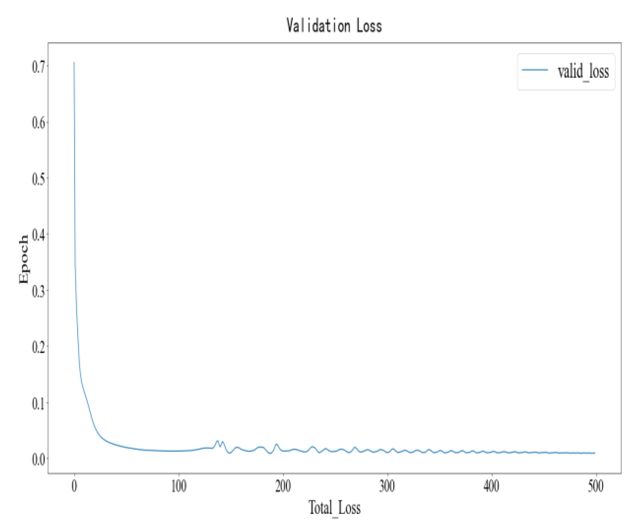
Figure 9 and Figure 10, respectively, describe the loss change process of each round of LSTM in the training set and verification set, where the abscx axis represents the epoch of training rounds, with a total of 500 rounds of training; the ordinate represents the total training error of each round, namely the summary value of the mean square error of each round. It can be seen that when the training reaches about 20 rounds, the model can simulate the samples in the training set very well, that is, better parameters are obtained in the training set.

4.3. WGAN Pricing Model

4.3.1. Model Description

As explained in the theory part of Section 2, WGAN, as a derivative model of basic GAN, inherits the advantages of the former, strengthens the training stability of the model and is widely used in the industry. Due to the special structure of the dual training model of WGAN, this paper refers to the modeling method of Kang (2019). It intends to use its discriminator to enhance the pricing effect of the generator model. The structure of the model is shown as follows in Figure 11:

(1)

Generator structure

As LSTM has many parameters, this section adopts the gated cycle unit structure (GRU) with faster computing performance as WGAN’s generator model, and uses Leaky ReLU as the activation function. The specific parameters are listed in the following table:

(2)

Discriminator structure

Compared with traditional GAN, the discriminator of WGAN cancels the Sigmoid activation function of the output layer, resulting in the final output not being a value between 0 and 1. Instead, the W distance between the generated distribution and the real distribution is fitted, thus making the training of the model more stable. This paper chooses a multi-layer perceptron as the discriminator of the WGAN model and Leaky ReLU as the activation function. The specific parameters are shown in the following table:

Where $f_w(x)$ represents the function satisfying the Lipschiz condition, which is replaced by the discriminator network model in this paper, $x^{\prime }~P_{fake\_data}$ represents the price sequence formed after adding the price generation result and $x~P_{data}$ represents the real price sequence. In particular, according to the practice of Arjovsky and Bottou (2017), the training frequency ratio of generator and discriminator is 1:5, that is, the discriminator model trains the generator model once every five times.

4.3.2. Empirical Results

In this empirical study, it can be seen that the pricing effect of test sample 1 (Jiangbank CB) is better in the first 1000 trading days, but higher in the last 150 trading days. On the whole, the MAPE of sample 1 is 0.806%, which is slightly higher than the 0.763% of the LSTM pricing model. However, for test sample 2 (SPD CB), the results of Figure 12, Figure 13 and MAPE (0.231%) are both better than the LSTM pricing model (0.3% MAPE) and the traditional LSM model (2.25% MAPE for multi-node duration), indicating that the application of WGAN helps to improve the pricing effect of the model.

As can be seen from the above empirical results, the LSTM model and WGAN model have a better pricing effect, and the average absolute error of the two training samples in the test set is less than 1%, which fully meets the pricing requirements. In addition, both of the two models are data-driven pricing models, mainly based on the sample data to be learned, rather than relying on the preconditions in other models. They are able to mine the nonlinear relationship in the data and adapt to the real market environment.

Next, this paper takes the method mentioned by Takahashi et al. (2019) as reference and Wiese et al. (2020) and Tan et al. (2022) as reference, and uses Quant GANs proposed by Wiese et al. (2020) to replace Monte Carlo as the generation model of stock price series. In order to improve the pricing effect of the model, it avoids the premise assumptions in the traditional model and reuses the unique statistical characteristics of financial data, such as leverage effect, coarse-fine volatility correlation and the gain/loss asymmetry of financial time series.

4.4. Improved Model of LSM

4.4.1. Model Description

The improved model of LSM in this paper adopts the Quant GANs model proposed by Wiese et al. (2020) as the generation model of stock price series, thus avoiding the assumptions in the traditional model, and then prices the convertible bonds according to the traditional LSM pricing method. Quant GANs is a financial time series generation model proposed by Wiese et al. (2020) in 2019.

4.4.2. Empirical Results

The selection of samples is consistent with the traditional LSM pricing model, and the first-day pricing of 17 samples of continued bonds is carried out. Among them, the training sample of the Quant GANs model adopts the stock price data of 17 samples of bonds, and the sample interval is from 1 January 2010 to 20 January 2023, which is representative after several bull and bear markets.

In order to make a horizontal comparison with the pricing results of other models, this paper also adopts the Shanghai Pudong Development convertible bond for multi-node pricing. The pricing method is consistent with the above, and the node selection method is consistent with that described in Section 4.1.4.

(1)

Generate sequence authenticity evaluation index

From the comparison of the following groups of figures, it can be intuitively seen that, except for the leverage effect, the generated sequence reproduces the style characteristics of the real sequence. In addition, it can be seen from Figure 14, Figure 15, Figure 16 and Figure 17 that the Quant GANs model can generate a return sequence basically consistent with the real sequence.

(2)

Pricing results of multi-node pricing within the duration

Consistent with the above, the multi-node pricing range of Shanghai Pudong Development convertible bonds is from 20 January 2022 to 20 January 2023, with 12 nodes every 30 days. The price of convertible bonds at each node is estimated, respectively, and the stock price volatility and stock price are updated every 30 days. Pricing results are shown in Figure 18 below:

Table 11. Pricing comparison of each model in details.

Date	Actual Price	LSM	Error Rate	LSTM	Error Rate	WGAN	Error Rate	LSM Improved	Error Rate
2022/2/21	105.90	102.76	−2.96%	106.36	0.43%	106.21	0.29%	106.89	0.93%
2022/3/21	104.72	102.14	−2.46%	104.97	0.24%	105.01	0.28%	104.51	−0.19%
2022/4/20	104.83	102.30	−2.40%	105.10	0.26%	105.02	0.18%	105.07	0.22%
2022/5/20	105.34	102.48	−2.71%	105.42	0.08%	105.35	0.01%	104.30	−0.99%
2022/6/20	105.07	102.84	−2.11%	105.20	0.13%	105.26	0.19%	104.38	−0.65%
2022/7/20	105.45	103.13	−2.19%	105.52	0.07%	105.51	0.05%	104.81	−0.61%
2022/8/22	106.30	103.30	−2.81%	106.61	0.30%	106.64	0.32%	103.80	−2.35%
2022/9/20	106.35	103.56	−2.62%	106.19	−0.15%	106.46	0.10%	104.06	−2.15%
2022/10/20	106.36	103.87	−2.34%	106.13	−0.21%	106.29	−0.06%	104.12	−2.10%
2022/11/21	105.37	102.86	−2.38%	105.23	−0.13%	105.38	0.01%	103.03	−2.22%
2022/12/20	104.01	103.23	−0.75%	104.27	0.25%	104.00	−0.01%	103.55	−0.44%
2023/1/20	104.91	103.54	−1.31%	105.21	0.28%	104.70	−0.21%	103.75	−1.10%
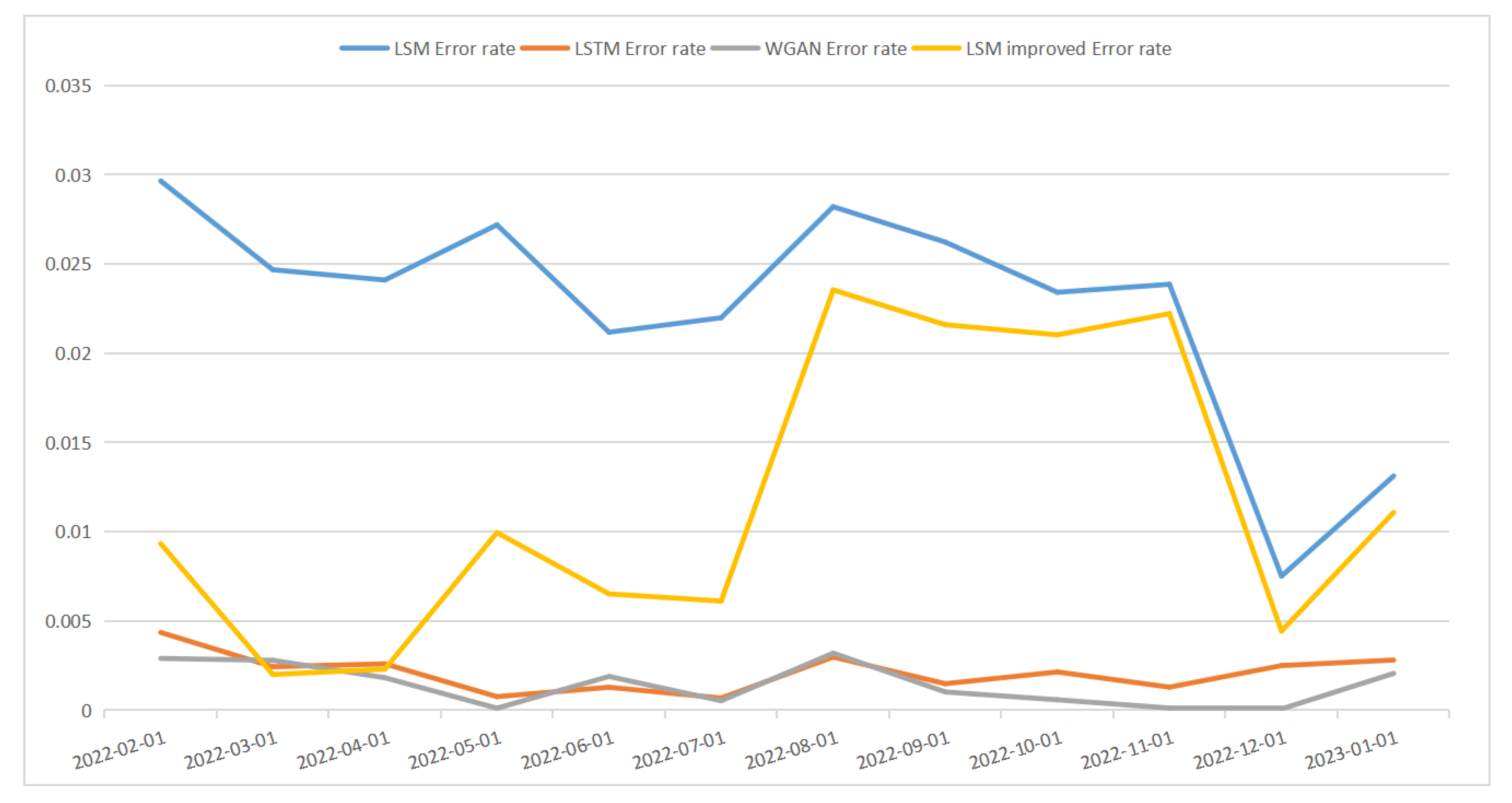
Mean	105.38	104.35	−2.26%	105.52	0.13%	105.49	0.10%	104.35	−0.98%

and Figure 19 show the pricing error rate of the four models, and the best pricing effect is the two deep learning models. From the perspective of the mean error rate, the pricing effect of WGAN (0.10%) is better than that of LSTM (0.13%), and the pricing effect of LSM’s improved model (−0.98%) is better than that of the traditional LSM model (−2.26%).

4.5. Comparative Analysis of Pricing Effect of Each Model

Due to the different pricing methods of each model, the scope of application of the model is also different. The traditional LSM can price convertible bonds at any time point, but the efficiency is low and the presupposition is not in line with the reality. The pure data-driven pricing model can achieve the purpose of improving the pricing effect by adding multiple characteristic variables describing the real situation. However, due to the model input problem, the price of the first day of listing of convertible bonds cannot be predicted. The improved model of LSM uses a data-driven approach to replace the generation of stock price trend sequence, so as to avoid the assumptions in the traditional model and meet the requirements that the generation sequence should meet the reality, but there are still requirements on the sample data of the underlying stock price of the convertible bond.

To sum up, this paper takes Shanghai Pudong Development Co., LTD as an example and uses error rate, MAPE and RMSE to evaluate the pricing effect of each model, as shown in

Table 12. Summary of pricing comparison of each model.

Model Name	MAPE	RMSE
LSM	2.26%	2.4699
LSTM	0.21%	0.2463
WGAN	0.14%	0.1902
LSM improved	1.17%	1.4895

.

Table 12 summarizes the MAPE value of each pricing model and describes the overall pricing effect of the model. It can be seen that the two deep learning models still have the best overall pricing effect, and the pricing effect of WGAN (MAPE 0.14%, RMSE 0.1902) is better than that of LSTM (MAPE 0.21%, RMSE 0.2463), and the pricing effect of LSM’s improved model (MAPE 1.17%, RMSE 1.4895) is better than that of the traditional LSM model (MAPE 2.26%, RMSE 2.4699).

5. Conclusions

This paper adopts the traditional LSM pricing model, and selects 17 bank convertible bonds that still exist on 20 January 2023 as pricing samples. The pricing method is the first day of listing pricing. In addition, in order to compare with other models, the Shanghai Pudong Development convertible bonds with higher pricing accuracy on the first day of listing are selected as the pricing samples of multi-node pricing within the duration. The pricing range is from 20 January 2022 to 20 January 2023, and there are 12 pricing nodes every 30 days. In the two data-driven models, the daily data of all maturing and unmaturing bank convertible bonds from 1 January 2012 to 20 January 2023 were selected as the sample data, with a total of 25 samples, totaling 18,134 sample values. Among them, 23 were selected as training sets, and the remaining two were selected as test sets (Jiangbank convertible bonds and Shanghai Pudong Development convertible Bonds) to test the pricing power of the model. It is worth noting that the characteristic variables of each sample point are obtained from the macro environment, the fundamentals of listed companies, bond base, options, convertible bond trading data and clause design according to the existing literature.

The improved LSM model mainly uses the Quant GANs model proposed by previouse researcher and scholoars as the generation model of stock price series, thus avoiding the assumptions in the traditional model, and then prices the convertible bond according to the traditional LSM pricing method. The pricing sample is consistent with the traditional LSM pricing model. The first day of listing pricing of 17 sample bonds and the multi-node pricing of Shanghai Development convertible bonds within the duration were all conducted. Among them, the training sample of the Quant GANs model adopted the stock price data of 17 sample bonds. The sample interval was from 1 January 2010 to 20 January 2023, after several bull and bear markets; the samples were representative.

By sorting out the empirical results of each model, we reach the following conclusions:

(1)

The traditional LSM pricing model has a large error in the first-day pricing, indicating that the pricing function of this model needs to be further improved;

(2)

Among the four pricing models, the LSTM pricing model and WGAN pricing model have the best pricing effect. From the perspective of the MAPE index, the pricing effect of the WGAN pricing model (0.14%) is better than that of the LSTM pricing model (0.21%), and the pricing effect of the LSM improved model (1.17%) is better than that of the traditional LSM model (2.26%);

(3)

Applying the generative deep learning model GAN to the pricing of convertible bonds can avoid strict assumptions and significantly improve the pricing effect of the traditional model.

Though there are some limitations of the existing research in this paper, the prospects for the future research direction are put forward also:

(1)

The factors affecting the pricing of convertible bonds can be selected more accurately and the prediction accuracy of the model can be improved;

(2)

Improve the Quant GANs model in the future, so that the generated samples can better reproduce the statistical characteristics of real sequences;

(3)

In order to avoid model failure on new data, we need to update the model in time and adjust and improve it according to new market conditions.

References

- Arjovsky, Martin, and Léon Bottou. 2017. Towards Principled Methods for Training Generative Adversarial Networks. arXiv arXiv:1701.04862. [Google Scholar]
- Batten, Jonathan A., Karren Lee-Hwei Khaw, and Martin R. Young. 2018. Pricing Convertible Bonds using Stochastic Interest Rate. Journal of Banking & Finance, S0378426618301006. [Google Scholar] [CrossRef]
- Brennan, Michael J., and Eduardo S. Schwartz. 1977. Convertible bonds: Valuation and optimal strategies for call and conversion. The Journal of Finance 32: 715–1699. [Google Scholar] [CrossRef]
- Chang, Jingwen, and Yongmao Wang. 2020. Pricing of Convertible Bonds Based on Tsallis Entropy Distribution under Stochastic Interest Rate Model. Operational Research and Management 29: 189–97, 231. [Google Scholar]
- Cox, John C., Stephen A. Ross, and Mark Rubinstein. 1979. Option pricing: A simplified approach. Journal of Financial Economics 7: 229–63. [Google Scholar] [CrossRef]
- Das, Sanjiv R., and Rangarajan K. Sundaram. 2007. An Integrated Model for Hybrid Securities. Management Science 53: 1439–51. [Google Scholar] [CrossRef]
- Dogariu, Mihai, Liviu-Daniel Ştefan, Bogdan Andrei Boteanu, Claudiu Lamba, and Bogdan Ionescu. 2021. Towards Realistic Financial Time Series Generation via Generative Adversarial Learning. Paper presented at 29th European Signal Processing Conference (EUSIPCO), Dublin, Ireland, August 23–27. [Google Scholar]
- Duan, Jin-Chuan. 1995. The GARCH Option Pricing Model. Mathematical Finance 1: 13–32. [Google Scholar] [CrossRef]
- Feng, Jianfen, Xuanyu Zhou, and Mengfei Duan. 2018. Design and Impact Analysis of Convertible Bond Option Terms. Management Review 30: 58–68. [Google Scholar]
- Feng, Yun, Bing-Hua Huang, and Yu Huang. 2016. Valuing resettable convertible bonds: Based on path decomposing. Finance Research Letters 19: 279–90. [Google Scholar] [CrossRef]
- Goodfellow, Ian, Jean Pouget-Abadie, Mehdi Mirza, Bing Xu, David Warde-Farley, Sherjil Ozair, Aaron Courville, and Yoshua Bengio. 2014. Generative Adversarial Networks. Advances in Neural Information Processing Systems 27: 2672. [Google Scholar]
- Gulrajani, Ishaan, Faruk Ahmed, Martin Arjovsky, Vincent Dumoulin, and Aaron C. Courville. 2017. Improved Training of Wasserstein GANs. arXiv arXiv:1704.00028. [Google Scholar]
- Hadad, Naama, Lior Wolf, and Moni Shahar. 2017. A Two-Step Disentanglement Method. Paper presented at Computer Vision and Pattern Recognition, Salt Lake City, UT, USA, June 18–22. [Google Scholar]
- Hull, John, and Alan White. 1988. The Use of the Control Variate Technique in Option Pricing. Journal of Financial and Quantitative Analysis 23: 237–51. [Google Scholar] [CrossRef]
- Hung, Mao-Wei, and Yan Wang Jr. 2002. Pricing Convertible Bonds Subject to Default Risk. Derivations 10: 75–87. [Google Scholar] [CrossRef]
- Ingersoll, Jonathan E., Jr. 1977. A contingent-claims valuation of convertible securities. Journal of Financial Economics 4: 289–321. [Google Scholar] [CrossRef]
- Kalotay, Andrew J., George O. Williams, and Frank J. Fabozzi. 1993. A Model for Valuing Bonds and Embedded Options. Financial Analysts Journal 49: 35–46. [Google Scholar] [CrossRef]
- Kang, Zhang. 2019. Stock Market Prediction Based on Generative Adversarial Network. Procedia Computer Science 147: 400–6. [Google Scholar]
- Koshiyama, Adriano, Firoozye Nick, and Philip Treleaven. 2021. Generative adversarial networks for financial trading strategies fine-tuning and combination. Quantitative Finance 21: 797–813. [Google Scholar] [CrossRef]
- Lai, Qinan, Changhui Yao, and Zhicheng Wang. 2005. An Empirical Study on the Pricing of Convertible Bonds in my country. Financial Research 9: 105–21. [Google Scholar]
- Lau, Ka Wo, and Yue Kuen Kwok. 2004. Anatomy of Option Features in Convertible Bonds. Journal of Futures Markets: Futures, Options, and Other Derivative Products 24: 513–32. [Google Scholar] [CrossRef]
- Longstaff, Francis A., and Eduardo S. Schwartz. 2001. Valuing American options by simulation: A simple least-squares approach. The Review of Financial Studies 14: 113–47. [Google Scholar] [CrossRef]
- Lvov, Dmitri, Ali Bora Yigitbasioglu, and Naoufel El Bachir. 2004. Pricing convertible bonds by simulation. Paper presented at Second IASTED International Conference, Clearwater Beach, FL, USA, November 28–December 1; pp. 259–64. [Google Scholar]
- Ma, Changfu, Wei Xu, and Xianzhi Yuan. 2019. Pricing Research on China’s Convertible Bonds Based on Two-Factor Willow. Systems Engineering Theory and Practice 39: 3011–23. [Google Scholar]
- Niu, Xiaojian, and Xiong Ba. 2021. Pricing and Empirical Analysis of Convertible Bonds Based on Machine Learning. Journal of the Party School of Guizhou Province 5: 58–71. [Google Scholar]
- Takahashi, Akihiko, Takao Kobayashi, and Naruhisa Nakagawa. 2001. Pricing convertible bonds with default risk: A Duffie-Singleton approach. Journal of Fixed Income 11: 20–29. [Google Scholar] [CrossRef]
- Takahashi, Shuntaro, Yu Chen, and Kumiko Tanaka-Ishii. 2019. Modeling financial time-series with generative adversarial networks. Physica A: Statistical Mechanics and its Applications 527: 121261. [Google Scholar] [CrossRef]
- Tan, Xiaoyu, Zili Zhang, Xuejun Zhao, and Shuyi Wang. 2022. DeepPricing: Pricing convertible bonds based on financial time-series generative adversarial networks. Financial Innovation (English) 8: 38. [Google Scholar] [CrossRef]
- Tang, Xiaobin, Manru Dong, and Rui Zhang. 2020. Research on Prediction of Consumer Confidence Index Based on Machine Learning LSTM&US Model. Statistical Research 37: 12. [Google Scholar]
- Tsiveriotis, Kostas, and Chris Fernandes. 1998. Valuing Convertible Bonds with Credit Risk. Journal of Fixed Income 8: 95–102. [Google Scholar] [CrossRef]
- Wiese, Magnus, Robert Knobloch, Ralf Korn, and Peter Kretschmer. 2020. Quant GANs: Deep Generation of Financial Time Series. Quantitative Finance 20: 1419–40. [Google Scholar] [CrossRef]
- Xie, Baishuai, Weiguo Zhang, Pingkang Liao, and Yana Chen. 2013. Pricing of Convertible Bonds with Credit Risk Based on Triangular Tree Model. Systems Engineering 31: 18–23. [Google Scholar]
- Xie, Yingbin. 2021. Research on Pricing of Convertible Bonds Based on Black-Scholes Model—Taking Oupai Convertible Bonds as an Example. China Price 11: 53–55. [Google Scholar]
- Yang, Changhui, Zhen Shao, Chen Liu, and Chao Fu. 2020. A Hybrid Modeling Method and Its Application in ETF Option Pricing. Chinese Management Science 28: 44–53. [Google Scholar]
- Yang, Jingyang, Yoon Choi, Shenghong Li, and Jinping Yu. 2010. A note on “Monte Carlo analysis of convertible bonds with reset clause”. European Journal of Operational Research 200: 924–25. [Google Scholar] [CrossRef]
- Yang, Xiaofeng, Jinping Yu, Mengna Xu, and Wenjing Fan. 2018. Convertible bond pricing with partial integro-differential equation model. Mathematics and Computers in Simulation 152: 35–50. [Google Scholar] [CrossRef]
- Yang, Yanli, and Hongyan Jiao. 2021. Insulator image generation method based on DCGAN. Automation and Instrumentation 36: 5–9. [Google Scholar]
- Yao, Xiao, Ke Li, and Le’an Yu. 2022. Research on Corporate Bond Default Risk Prediction Based on Generative Adversarial Network Oversampling Technology under Unbalanced Samples. Systems Engineering Theory and Practice 42: 18. [Google Scholar]
- Zhao, Yang, and Lichen Zhao. 2009. Research on Convertible Bond Pricing Based on Monte Carlo Simulation. Journal of Systems Engineering 24: 621–25. [Google Scholar]
- Zheng, Zhenlong, and Hai Lin. 2004. Research on the Pricing of Convertible Bonds in China. Journal of Xiamen University (Philosophy and Social Sciences Edition) 162: 93–99. [Google Scholar]
- Zhou, Wei, Meiying Yang, and Liyan Han. 2007. A Nonparametric Approach to Pricing Convertible Bond via Neural Network. Paper presented at Eighth ACIS International Conference on Software Engineering, Artificial Intelligence, Networking, and Parallel/Distributed Computing (SNPD 2007), Qingdao, China, July 30–August 1; vol. 2, pp. 564–69. [Google Scholar]
- Zhou, Zhengyi, and Chongfeng Wu. 2013. The impact of cash dividends and conversion price adjustments on the pricing of convertible bonds. Investment Research 32: 55–67. [Google Scholar]
Figure 1.
Research framework of the paper.
Figure 2.
Unrevised path.
Figure 3.
Downward revision path.
Figure 4.
LSTM structure diagram.
Figure 5.
Structure diagram of GAN model.
Figure 6.
Distribution of real data and generated data during training.
Figure 7.
Yield distribution of convertible bonds and shares of Jiangbank.
Figure 8.
Multi-node pricing chart of Shanghai Pudong Development Co., LTD.
Figure 9.
Loss diagram of training set.
Figure 10.
Loss diagram of verification set.
Figure 11.
Structure of WGAN pricing model.
Figure 12.
LSTM model pricing effect of test sample 1.
Figure 13.
Pricing effect of WGAN model of test sample 1.
Figure 14.
Real sequence feature diagram.
Figure 15.
Generated sequence feature diagram.
Figure 16.
Real sequence rate of return.
Figure 17.
Generate a sequence yield graph.
Figure 18.
Multi-section pricing chart of Shanghai Pudong Development convertible bond.
Figure 19.
Multi-node pricing error rate of each model.