
A Level Set Analysis and A Nonparametric Regression on S&P 500 Daily Return


Abstract
:1. Introduction
2. Level Set Analysis
3. Nonparametric Regression
3.1. Local Polynomial Regression
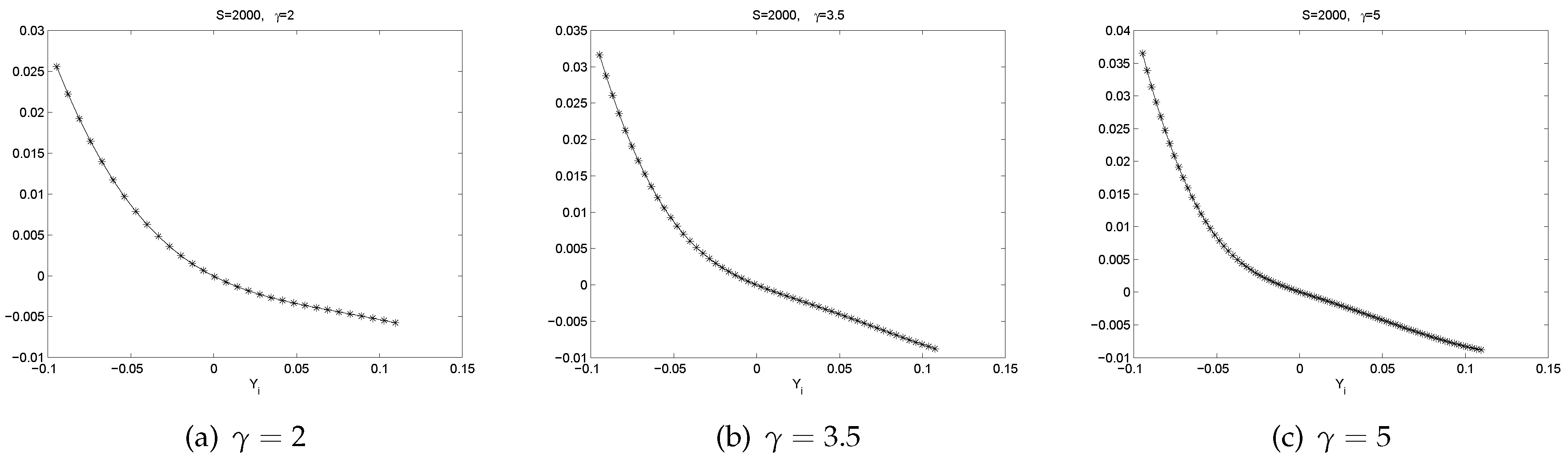
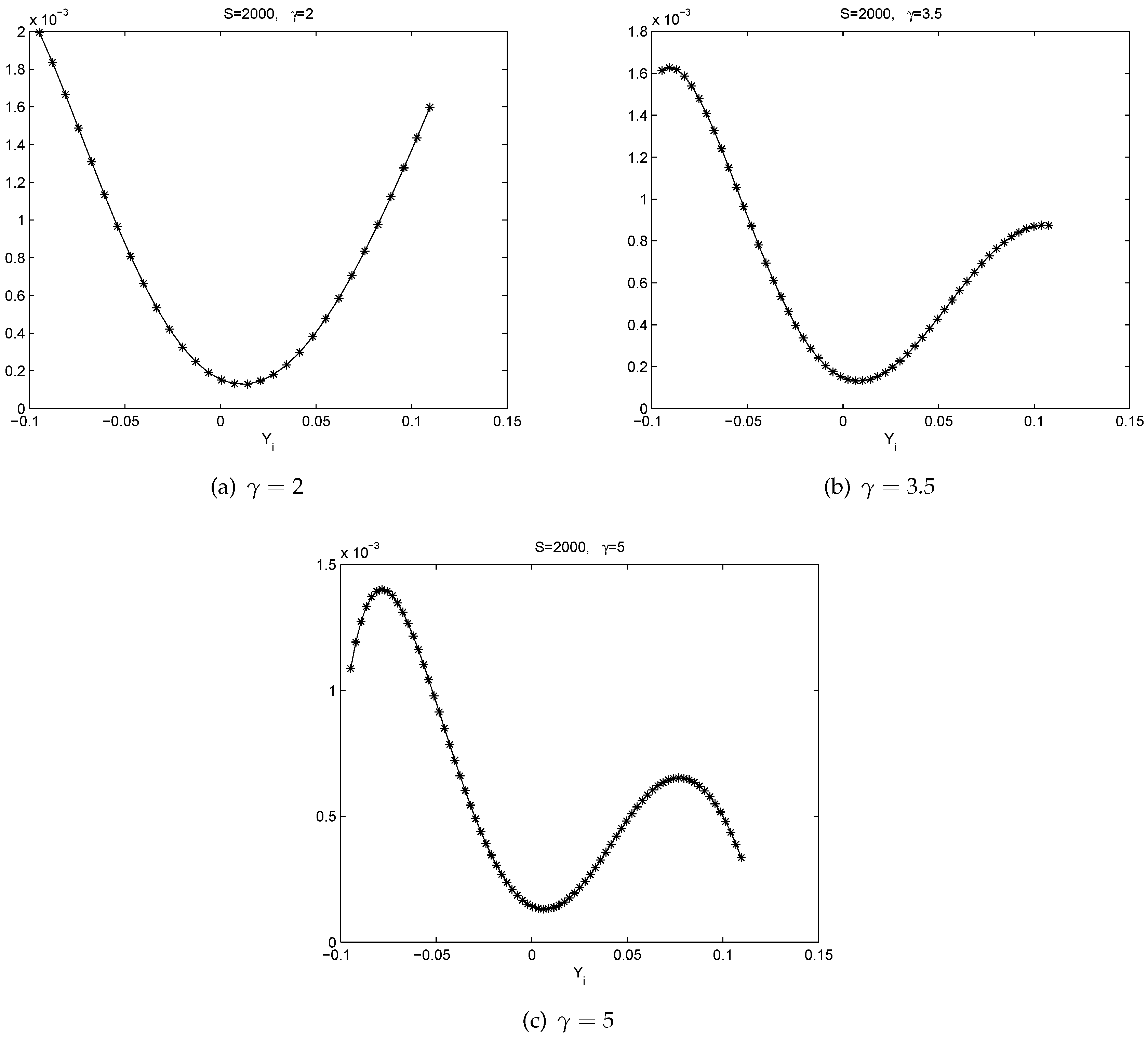
- There is a pattern of . If , is slightly negative. If , is positive. This represents a mean reverting pattern, or negative serial correlation on .
- If is large, i.e., there is a big gain at time , then on expectation, tends to be slightly negative. However, if is large negative, then on expectation, tends to be largely positive. So, there is an obvious bend in the curve of .
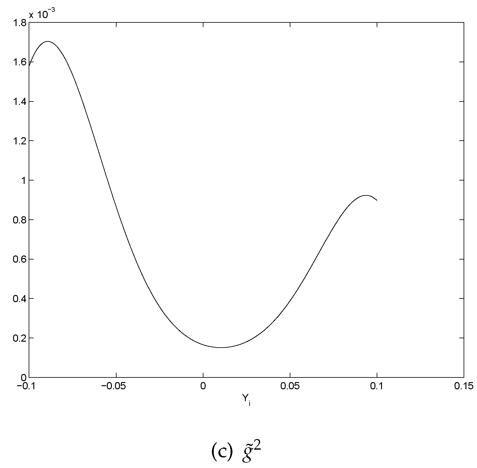
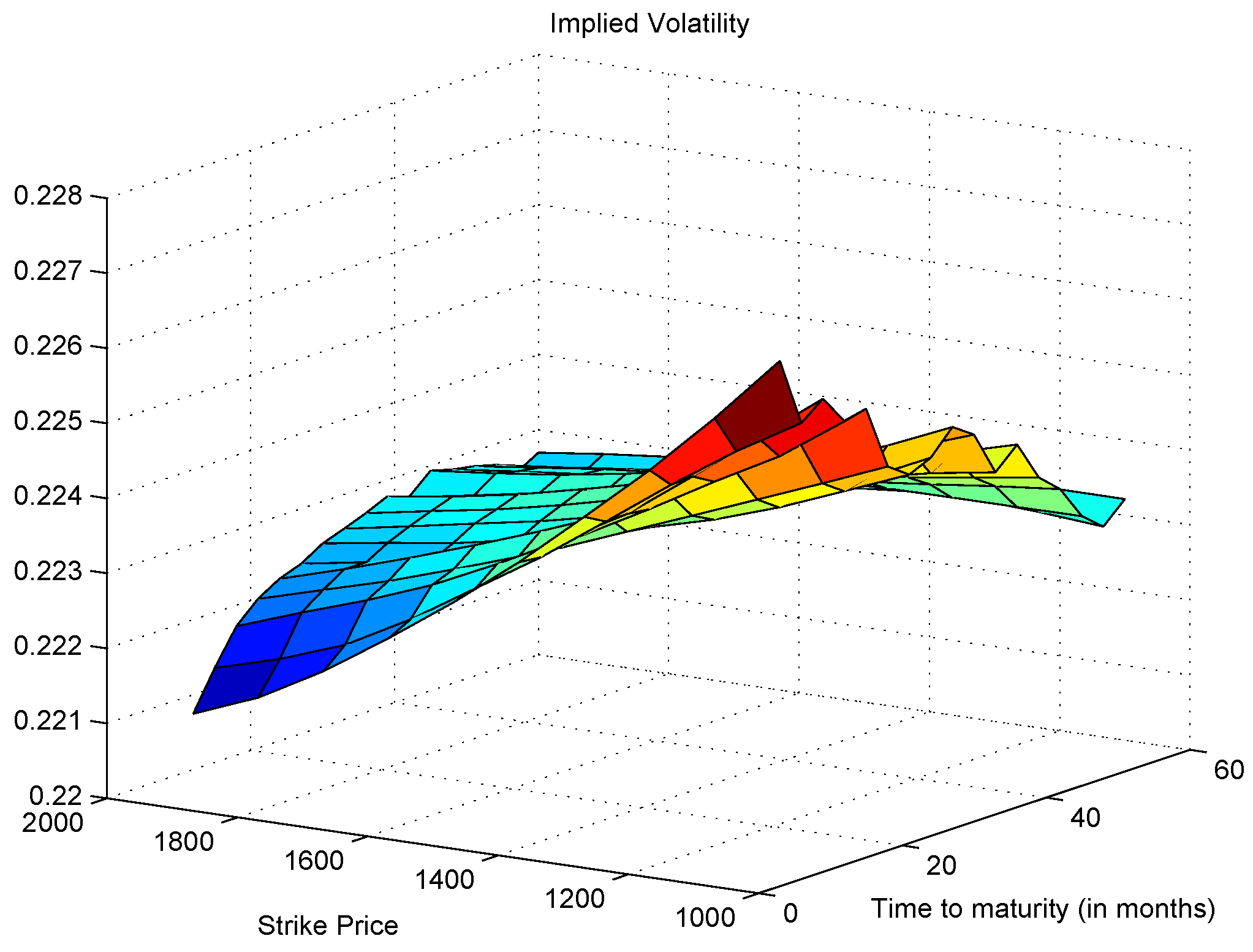
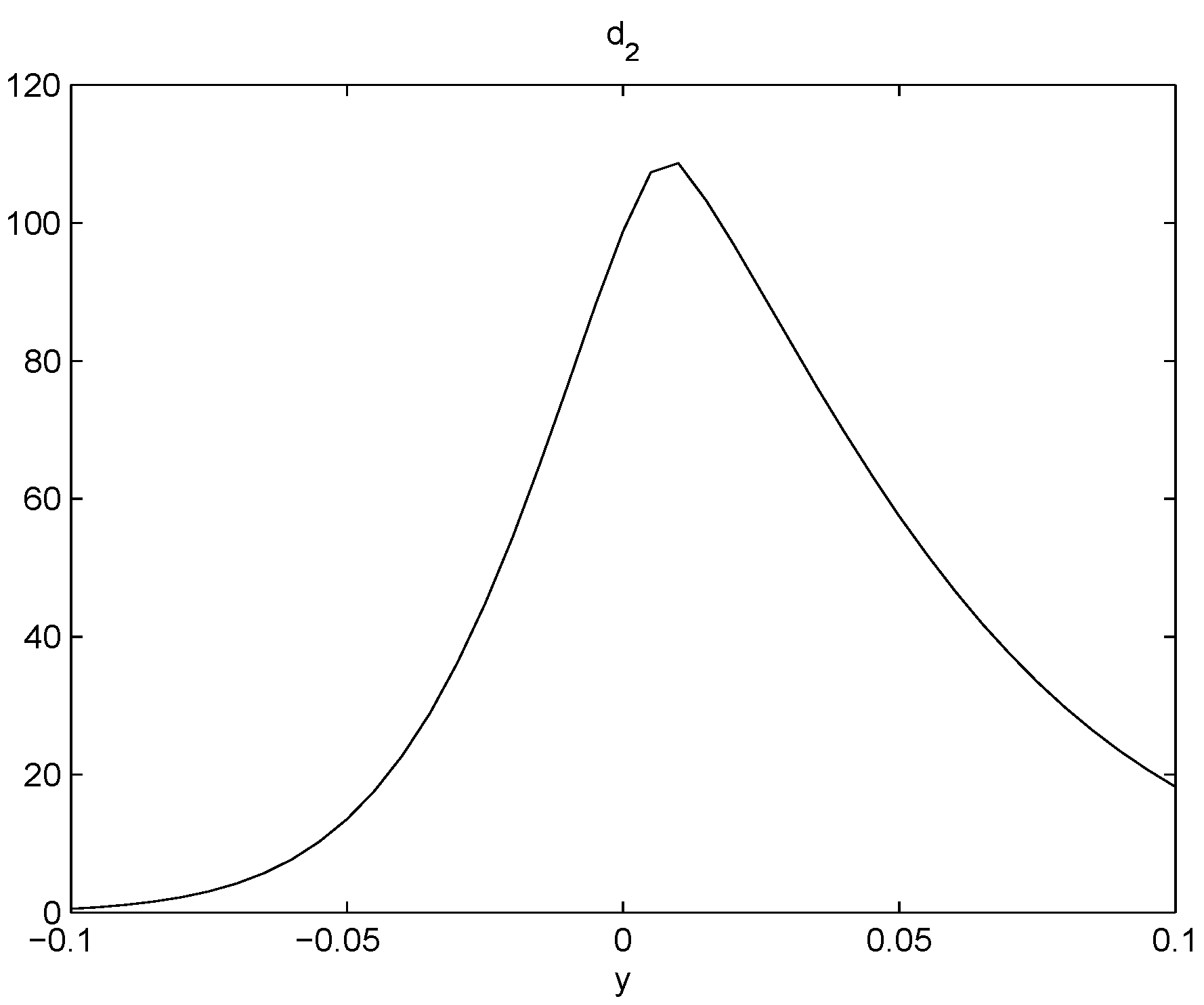
- All the graphs of show U-shaped “smiling faces”, and the minimum is achieved at a point of close to zero. In fact, a point that is slightly to the right of zero. Thus, large magnitude of corresponds to large volatility. What is more, on each “smiling face”, the left side of the curve is higher than the right side of the curve. Thus, these are tilted “smiling faces”, or skew.
- When γ is big, we observe the boundary effect on the boundaries of the interval, see, e.g., the graphs of . This phenomenon was also observed in [26] where an explanation was provided.
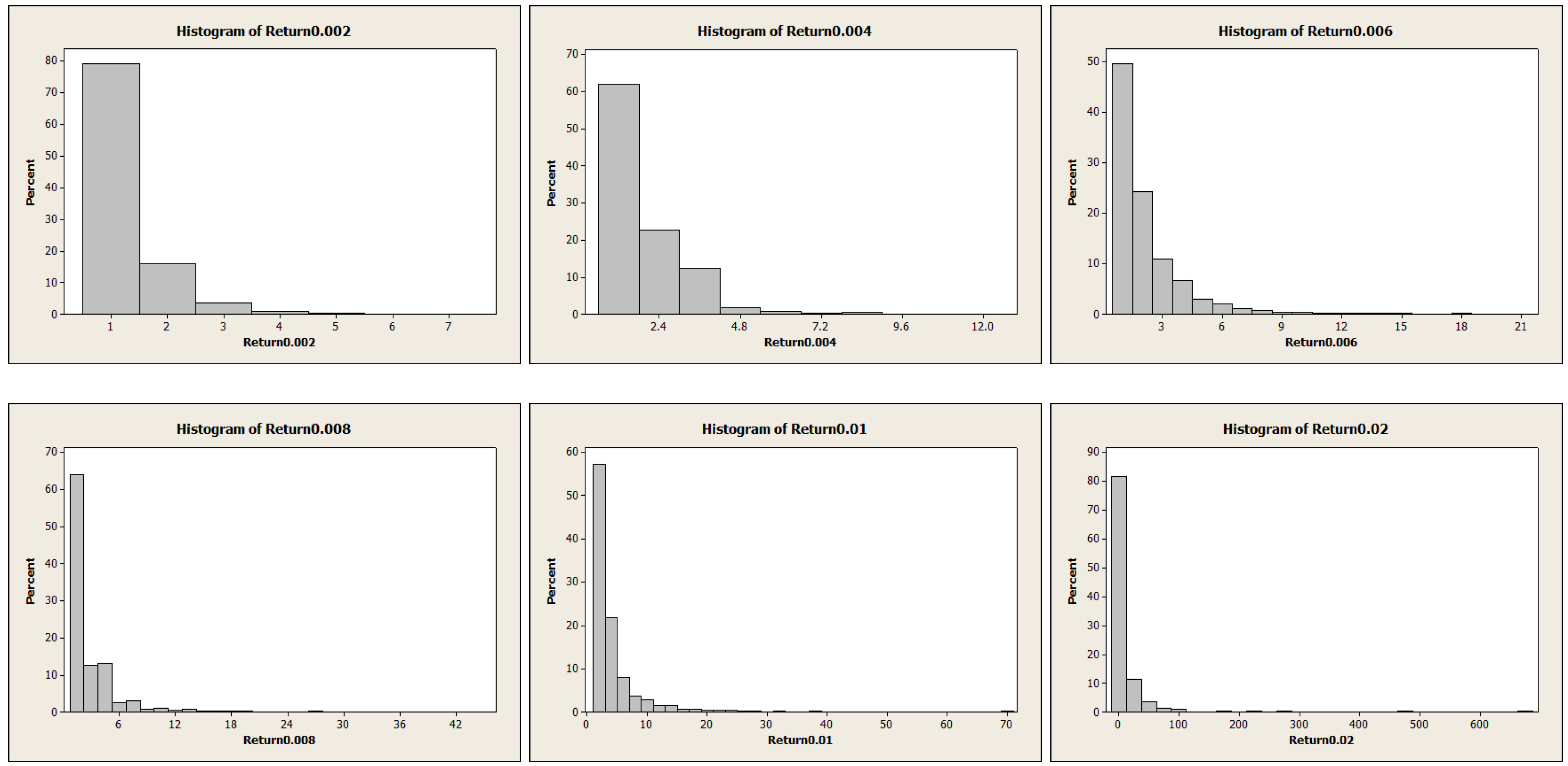
- These discoveries are pretty robust in view of various data sizes.
3.2. An ARCH Model
3.3. Model Comparison
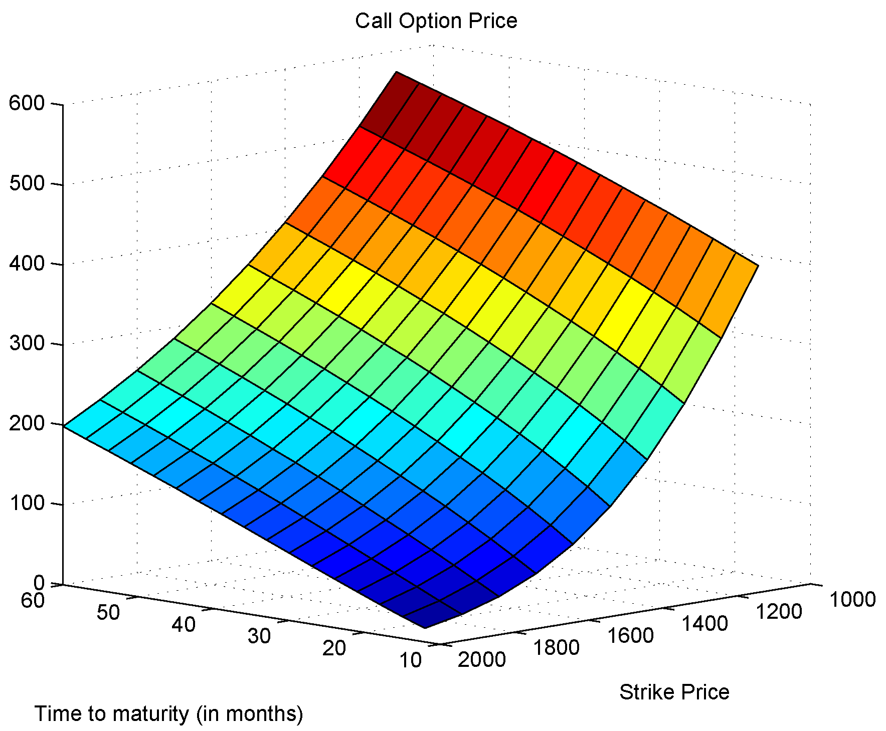
3.4. Option Pricing and Implied Volatility
4. Price Fluctuation and Market Participants
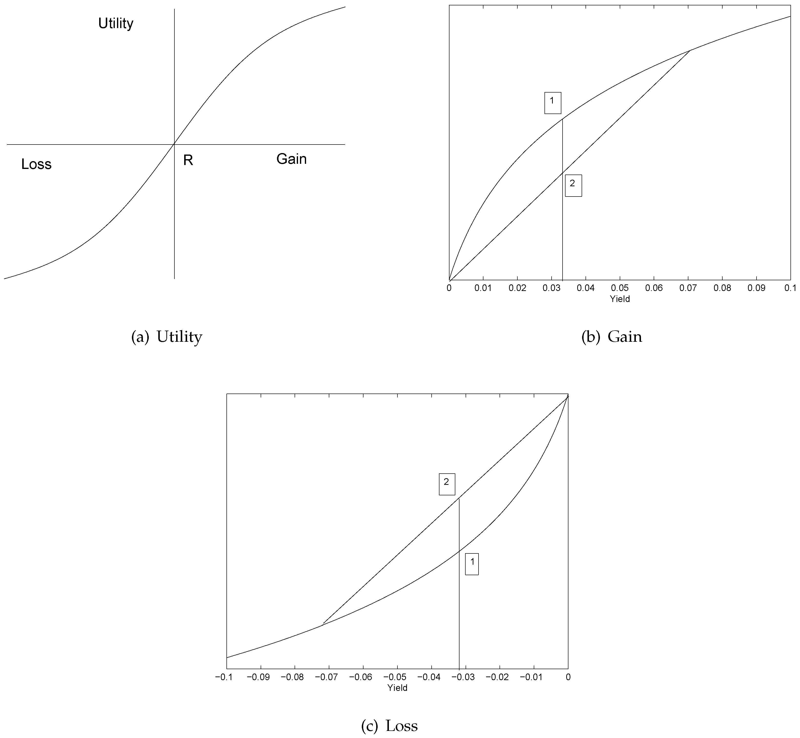
4.1. Prospect Agents
4.2. An ARCH Model from Prospect Theory
5. Conclusions
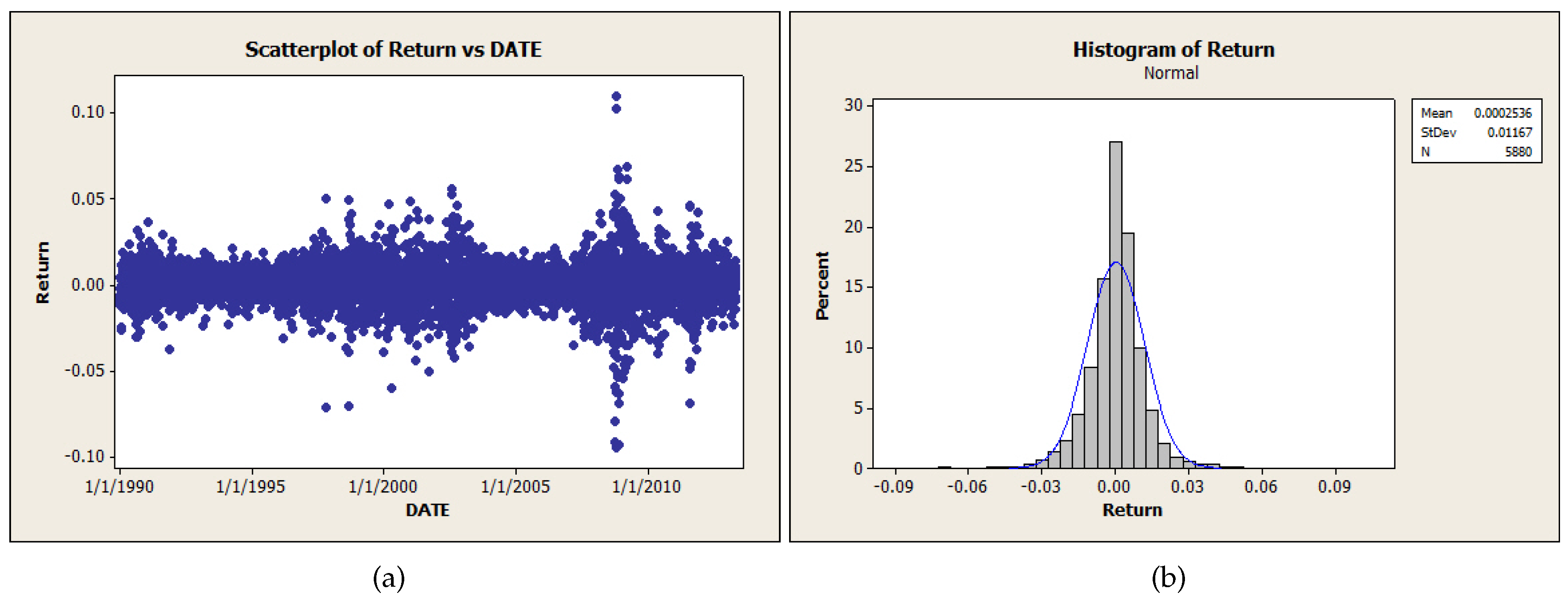
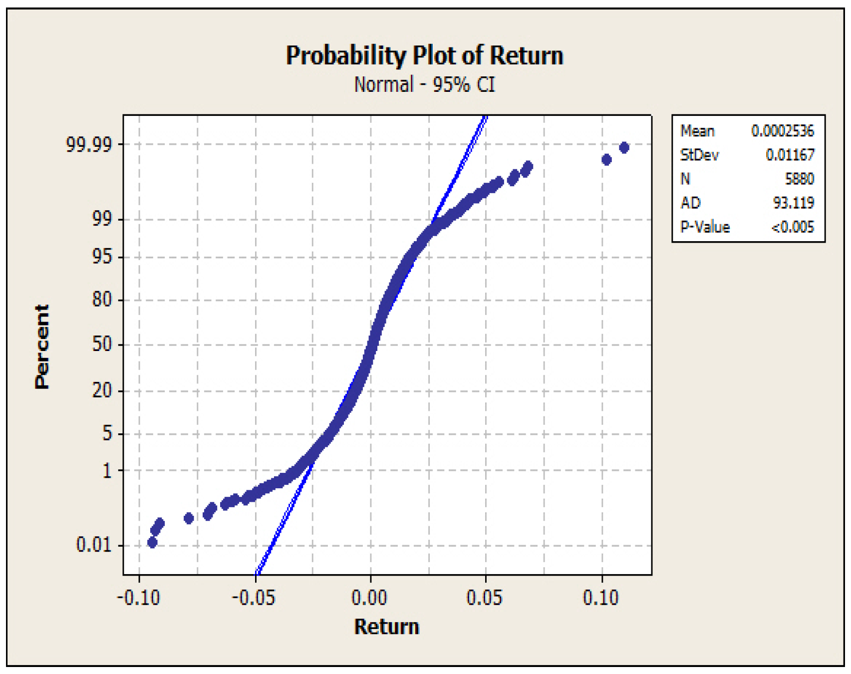
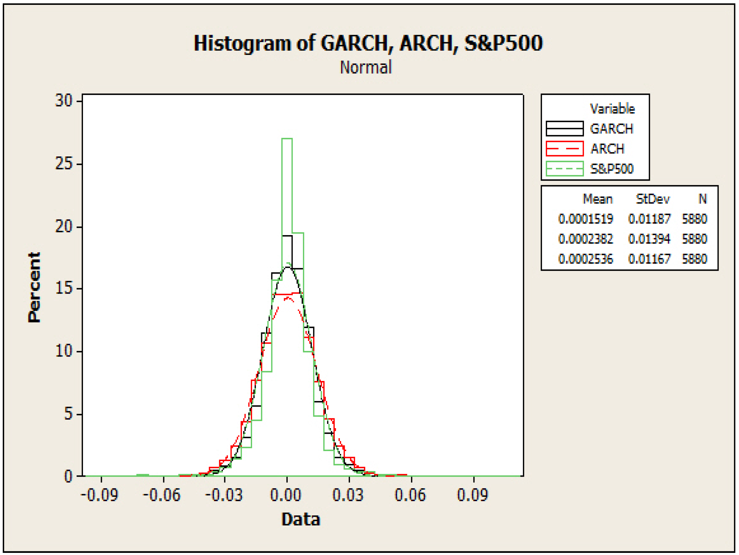
- We proposed a level set analysis and performed a nonparametric analysis on the S&P 500 return, and the results showed that this return process has negative serial correlation and volatility clustering property.
- We found new patterns on the S&P 500 return through local polynomial regression and constructed an ARCH model that replicates both the drift and volatility terms.
- We brought in the prospect theory to explain the mechanism of our model and linked it to the volatility skew phenomenon observed in the actual stock market.
Acknowledgments
Author Contributions
Conflicts of Interest
References
- R. Engle. “Autoregressive Conditional Heteroskedasticity with Estimates of the Variance of U.K. Inflation.” Econometrica 50 (1982): 987–1008. [Google Scholar] [CrossRef]
- T. Bollerslev. “Generalized Autoregressive Conditional Heteroscedasticity.” J. Econom. 31 (1986): 307–327. [Google Scholar] [CrossRef]
- E. Jacquier, N.G. Polson, and P.E. Rossi. “Bayesian Analysis of Stochastic Volatility Models.” J. Bus. Econ. Stat. 12 (1994): 371–417. [Google Scholar]
- S.J. Taylor. “Financial Returns Modelled by the Product of Two Stochastic Processes-A Study of Daily Sugar Prices, 1961–1979.” In Time Series Analysis: Theory and Practice. Edited by O.D. Anderson. New York, NY, USA: Elsevier/North-Holland, 1982, Volume 1, pp. 203–226. [Google Scholar]
- J.P. Fouque, G. Papanicolaou, and K.R. Sircar. Derivatives in Financial Markets with Stochastic Volatility. Cambridge, UK: Cambridge University Press, 2000. [Google Scholar]
- N. Shephard. “Statistical Aspects of ARCH and Stochastic Volatility.” In Time Series Models in Econometrics, Finance and Other Fields. Edited by D.R. Cox, D.V. Hinkley and O.E. Barndorff-Nielson. London, UK: Chapman and Hall, 1996, pp. 1–100. [Google Scholar]
- O.E. Barndorff-Nielsen, and N. Shephard. “Non-Gaussian Ornstein-Uhlenbeck-based models and some of their uses in financial economics.” J. R. Stat. Soc. Ser. B Stat. Methodol. 63 (2001): 167–241. [Google Scholar] [CrossRef]
- O.E. Barndorff-Nielsen, and N. Shephard. “Modelling by Lévy Processes for Financial Econometrics.” In Lévy Processes: Theory and Applications. Edited by O.E. Barndorff-Nielsen, T. Mikosch and S. Resnick. New York, NY, USA: Birkhäuser, 2001, pp. 283–318. [Google Scholar]
- J. Rosiński. “Tempering stable processes.” Stoch. Process Appl. 117 (2007): 677–707. [Google Scholar] [CrossRef]
- R.S. Tsay. Analysis of Financial Time Series, 3rd ed. Hoboken, NJ, USA: John Wiley and Sons, 2010. [Google Scholar]
- E. Bayraktar, H.V. Poor, and K.R. Sircar. “Estimating the Fractal Dimension of the S&P500 Index Using Wavelet Analysis.” Int. J. Theor. Appl. Financ. 7 (2004): 615–643. [Google Scholar]
- J. McCarthy, and A.G. Orlov. “Time-frequency Analysis of Crude Oil and S&P500 Futures Contracts.” Quant. Financ. 12 (2012): 1893–1908. [Google Scholar]
- R. Becker, J. Lee, and B.E. Gup. “An Empirical Analysis of Mean Reversion of the S&P500’s P/E Ratio.” J. Econ. Financ. 36 (2012): 675–690. [Google Scholar]
- Y.S. Kim, S.T. Rachev, M.L. Bianchi, I. Mitov, and F.J. Fabozzi. “Time series analysis for financial market meltdowns.” J. Bank. Financ. 35 (2011): 1879–1891. [Google Scholar] [CrossRef]
- N.P.B. Bollen. “Valuing Options in Regime-Switching Models.” J. Deriv. 6 (1998): 38–49. [Google Scholar] [CrossRef]
- A. Papanicolaou, and R. Sircar. “A Regime-Switching Heston Model for VIX and S&P 500 Implied Volatilities.” Quant. Financ. 14 (2013): 1811–1827. [Google Scholar]
- H. Chen, G. Noronha, and V. Singal. “The Price Response to S&P 500 Index Additions and Deletions: Evidence of Asymmetry and a New Explanation.” J. Financ. 59 (2004): 1901–1930. [Google Scholar]
- H. Föllmer, and M. Schweizer. “A Microeconomic Approach to Diffusion Models for Stock Prices.” Math. Financ. 3 (1993): 1–23. [Google Scholar] [CrossRef]
- U. Horst. “Financial Price Fluctuations in A Stock Market Model with Many Interacting Agents.” Econ. Theory 25 (2005): 917–932. [Google Scholar] [CrossRef]
- R. Frey, and A. Stremme. “Market Volatility and Feedback Effects from Dynamic Hedging.” Math. Financ. 7 (1997): 351–374. [Google Scholar] [CrossRef]
- P. Heemeijer, C. Homoes, J. Sonnemans, and J. Tuinstra. “Price Stability and Volatility in Markets with Positive and Negative Expectations Feedback: An Experimental Investigation.” J. Econ. Dyn. Control 33 (2009): 1052–1072. [Google Scholar] [CrossRef]
- A. Danilova. “Emergence of Stochastic Volatility from Informational Heterogeneity.” Doctoral Dissertation, Princeton University, Princeton, NJ, USA, 2005. [Google Scholar]
- G. Lyengar, and A.K.C. Ma. “A Behavioral Finance-based Tick-by-tick Model for Price and Volume.” J. Comput. Financ. 14 (2010): 57–80. [Google Scholar]
- E. Platen, and M. Schweizer. “On Feedback Effects from Hedging Derivatives.” Math. Financ. 8 (1998): 67–84. [Google Scholar] [CrossRef]
- D. Kahneman, and A. Tversky. “Prospect Theory: An Analysis of Decision under Risk.” Econometrica 47 (1979): 263–292. [Google Scholar] [CrossRef]
- W. Härdle, and A.B. Tsybakov. “Local Polynomial Estimators of the Volatility Function in Nonparametric Autoregression.” J. Econom. 81 (1997): 223–242. [Google Scholar] [CrossRef]
- E. Masry, and J. Fan. “Local Polynomial Estimation of Regression functions for mixing processes.” Scand. J. Stat. 24 (1997): 165–179. [Google Scholar] [CrossRef]
- W.S. Cleveland. “Robust Locally Weighted Regression and Smoothing Scatterplots.” J. Am. Stat. Assoc. 74 (1979): 829–836. [Google Scholar] [CrossRef]
- T. Bollerslev, U. Kretschmer, C. Pigorsch, and G. Tauchen. “A Discrete-time Model for Daily S&P 500 Returns and Realized Variations: Jumps and Leverage Effects.” J. Econom. 150 (2009): 151–166. [Google Scholar]
- P. Christoffersen, B. Feunou, and Y. Jeon. “Option Valuation with Observable Volatility and Jump Dynamics.” J. Bank. Financ. 61 (2015): S101–S120. [Google Scholar] [CrossRef]
- M.C. Mariani, I. SenGupta, and G. Sewell. “Numerical methods applied to option pricing models with transaction costs and stochastic volatility.” Quant. Financ. 15 (2015): 1417–1424. [Google Scholar] [CrossRef]
- I. SenGupta. “Option pricing with transaction costs and stochastic interest rate.” Appl. Math. Financ. 21 (2014): 399–416. [Google Scholar] [CrossRef]
- F.B. Slimane, M. Mehanaoui, and I.A. Kazi. “How Does the Financial Crisis Affect Volatility Behavior and Transmission Among European Stock Markets? ” Int. J. Financ. Stud. 1 (2013): 81–101. [Google Scholar] [CrossRef] [Green Version]
- B.M. Barber, and T. Odean. “The Behavior of Individual Investors.” In Handbook of the Economics of Finance. Edited by G.M. Constantinides, M. Harris and R.M. Stulz. North-Holland, The Netherlands: Elsevier, 2013, Volume 2, pp. 1533–1570. [Google Scholar]
- H. Shefrin, and M. Statman. “The Disposition to Sell Winners Too Early and Ride Losers Too Long: Theory and Evidence.” J. Financ. 40 (1985): 777–790. [Google Scholar] [CrossRef]
- A. Fiegenbaum, and H. Thomas. “Attitudes Toward Risk and the Risk-Return Paradox: Prospect Theory Explanations.” Acad. Manag. J. 31 (1988): 85–106. [Google Scholar] [CrossRef]
- T. Odean. “Are Investors Reluctant to Realize Their Losses? ” J. Financ. 53 (1998): 1775–1798. [Google Scholar] [CrossRef]
- J. Yao, and D. Li. “Prospect Theory and Trading patterns.” J. Bank. Financ. 37 (2013): 2793–2805. [Google Scholar] [CrossRef]


| Variable | Obs | Mean | SE Mean | StDev | Median | Skewness |
|---|---|---|---|---|---|---|
| Ret-ex | 5880 | –0.000000 | 0.000152 | 0.011669 | 0.000279 | –0.23 |
| Return0.002 | 4595 | –0.000005 | 0.000195 | 0.013186 | 0.002211 | –0.20 |
| Return0.004 | 3516 | –0.000042 | 0.000253 | 0.014983 | 0.004263 | –0.17 |
| Return0.006 | 2683 | –0.000226 | 0.000327 | 0.016924 | 0.006083 | –0.13 |
| Return0.008 | 2055 | –0.000428 | 0.000418 | 0.018944 | 0.008007 | –0.09 |
| Return0.01 | 1570 | –0.000786 | 0.000532 | 0.021086 | –0.010137 | –0.04 |
| Return0.02 | 434 | –0.00250 | 0.00158 | 0.03291 | –0.02081 | 0.09 |
| Return0.03 | 152 | –0.00317 | 0.00366 | 0.04506 | –0.03031 | 0.09 |
| Return0.04 | 59 | –0.00645 | 0.00757 | 0.05815 | –0.04268 | 0.19 |
| Return0.05 | 28 | –0.0183 | 0.0129 | 0.0684 | –0.0540 | 0.63 |
| Return0.06 | 18 | –0.0165 | 0.0183 | 0.0775 | –0.0633 | 0.53 |
| Return0.07 | 8 | –0.0364 | 0.0312 | 0.0883 | –0.0754 | 1.39 |
| Return0.08 | 5 | –0.0139 | 0.0489 | 0.1093 | –0.0923 | 0.61 |
| Return0.09 | 5 | –0.0139 | 0.0489 | 0.1093 | –0.0923 | 0.61 |
| Return0.1 | 2 | 0.10576 | 0.00356 | 0.00503 | 0.10576 | N/A |
| Variable | Return | Return0.002 | Return0.004 | Return0.006 | Return0.008 |
|---|---|---|---|---|---|
| DW | 2.11692 | 2.10942 | 2.08167 | 2.11201 | 2.11218 |
| Variable | Return0.01 | Return0.02 | Return0.03 | Return0.04 | Return0.05 |
| DW | 2.13184 | 2.20106 | 2.05984 | 2.75493 | 2.23021 |
| Variable | Return | Return0.002 | Return0.004 | Return0.006 | Return0.008 |
|---|---|---|---|---|---|
| DW | 2.27197 | 2.25019 | 2.25131 | 2.32910 | 2.34118 |
| Obs | 505 | 446 | 385 | 335 | 290 |
| Variable | Return0.01 | Return0.02 | Return0.03 | Return0.04 | Return0.05 |
| DW | 2.36018 | 2.28681 | 2.02110 | 2.51461 | 2.60353 |
| Obs | 249 | 126 | 64 | 38 | 21 |
| Variable | Return | Return0.002 | Return0.004 | Return0.006 | Return0.008 |
|---|---|---|---|---|---|
| DW | 2.22249 | 2.23713 | 2.23029 | 2.21794 | 2.22877 |
| Obs | 5880 | 5192 | 4497 | 3807 | 3166 |
| Variable | Return0.01 | Return0.02 | Return0.03 | Return0.04 | Return0.05 |
| DW | 2.18704 | 2.19967 | 2.26081 | 2.10487 | 2.06198 |
| Obs | 2638 | 821 | 213 | 53 | 16 |
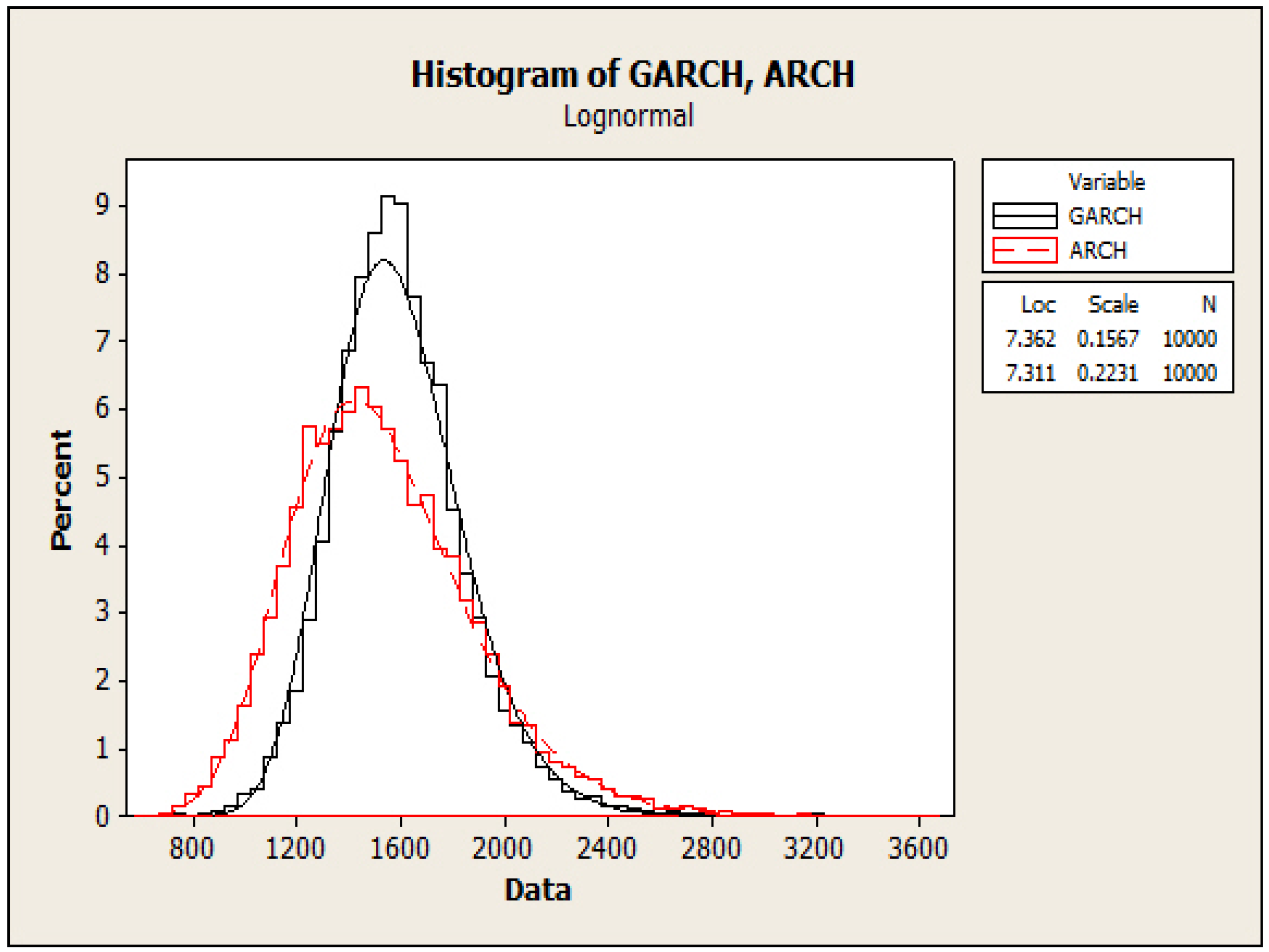
| Model | N | Mean | SE-Mean | StDev | Minimum | Q1 | Median | Q3 | Maximum | Skewness |
|---|---|---|---|---|---|---|---|---|---|---|
| GARCH | 10,000 | 1593.9 | 2.54 | 253.8 | 703.9 | 1427.7 | 1573.2 | 1736.0 | 3670.0 | 0.78 |
| ARCH | 10,000 | 1533.7 | 3.45 | 345.1 | 606.7 | 1284.9 | 1497.6 | 1739.5 | 3170.0 | 0.65 |
© 2016 by the authors; licensee MDPI, Basel, Switzerland. This article is an open access article distributed under the terms and conditions of the Creative Commons by Attribution (CC-BY) license (http://creativecommons.org/licenses/by/4.0/).
Share and Cite
Yang, Y.; Tsoi, A. A Level Set Analysis and A Nonparametric Regression on S&P 500 Daily Return. Int. J. Financial Stud. 2016, 4, 3. https://doi.org/10.3390/ijfs4010003
Yang Y, Tsoi A. A Level Set Analysis and A Nonparametric Regression on S&P 500 Daily Return. International Journal of Financial Studies. 2016; 4(1):3. https://doi.org/10.3390/ijfs4010003
Chicago/Turabian StyleYang, Yipeng, and Allanus Tsoi. 2016. "A Level Set Analysis and A Nonparametric Regression on S&P 500 Daily Return" International Journal of Financial Studies 4, no. 1: 3. https://doi.org/10.3390/ijfs4010003