Value Investing and Size Effect in the South Korean Stock Market


Departamento de Metodos Cuantitativos, University of Granada, 18010 Granada, Spain
Int. J. Financial Stud. 2018, 6(1), 31; https://doi.org/10.3390/ijfs6010031
Submission received: 18 December 2017
/
Revised: 14 February 2018
/
Accepted: 28 February 2018
/
Published: 12 March 2018
Abstract
:There are indications that value investing strategies have been able to outperform the overall market in several countries across the globe. In this article, the specific case of South Korea is analyzed. It would appear that from a rigorous statistical point of view there are no strong evidence supporting the outperformance of value stocks versus growth stocks in South Korea, particularly when measured on a yearly basis. These results were consistent using both MSCI value and growth indexes as well as constructing portfolios using the P/E, P/B, cash flow per share and average 5-year sales growth. The statistical tests performed failed to reject for the majority of the years that the monthly returns come from distributions with different medians. The test yielding rather consistent results on a yearly basis but for large periods of time (decades) the results were more mixed, pointing in some cases to value investing outperforming over that very long time frame. It should be noted that the final value of the portfolios was rather different when using criteria, such as low P/E, typically associated with value stocks. The tests also failed to reject the hypothesis of different means for the monthly returns of small, medium and large companies.
1. Introduction
The idea that value investing in the long term outperforms other strategies, such as growth investment, is a widely held assumption by many institutional investors but the bulk on the research on this topic has focused on the U.S. case which is a mature market of an enormous size compared to most other countries. In simple terms value stocks are those that have relatively low valuations while having relatively stable business with typically low growth rates. Growth stocks are those that have high growth rates, compared to the overall market and hence are perceived by supporters of this technique as desirable stocks. Another commonly found feature in some markets is the small size effect. In some countries such as the U.S. it has been shown that companies with relatively small market capitalization tend to outperform large companies. More details in these two effects will be explained in later sections of these article.
Extrapolating the results regarding the value and small size effect from articles mostly covering the U.S. into other countries might yield inaccurate results. In this article, the specific case of South Korea is analyzed. South Korea, as will be explained later in this article, is a rather unique country with features typically associated with developed countries, such as relatively high GDP per capita, to other features more common in emerging markets such as questionable corporate governance (Gupta 2014) associated with some of its largest family conglomerates. These family conglomerates are commonly called using the Korean term chaebol and form the backbone of the Korean economy. A peculiarity of these chaebols is that they often include an intricate ownership structure (Choi and Kang 2014) as well as cross holdings in other chaebols, which could in turn distort some of the stock prices of the related companies. The impact of these chaebols on the economy has been debated (Premack 2017; Chiang 2017) with mixed views. Needless to say, that South Korea also faces a very unique geopolitical situation with continued tensions with North Korea. This is a conflict that it has prolonged for decades with the two Koreas actually formally remaining at war. Tensions seem to have escalated in recent times and this could be another rather specific factor potentially affecting South Korean stock prices. Another interesting characteristic of the South Korean case is how quickly the country passed from being an underdeveloped country to become arguable a developed economy and a member of the G20 in what is sometimes referred as the South Korean Miracle. Given the size of the Korean economy as well as its peculiarities, such as the cross holdings of chaebols, it is not possible a priori to assume that the behaviours found in another stock exchanges, such as the outperformance of value stocks, would necessarily apply to this market. It would appear therefore necessary to perform a detailed analysis to ascertain if this effect is actually present in the Korean market.
This article has two main objectives. The first one is to determine, using historical performance, if the stock market in South Korea presents the value effect or in other words if value stocks outperform. The null hypothesis is that there is no value effect in the South Korean stock market. The existence of a value effect is important in the context of decision making for investments, applying the concept of value investing to a market such as South Korea in a naïve way without making further tests confirming the existence of a value effect could lead to unwanted investment results. It would be shown in this article that while at a first glance it would appear to exist a value effect in the South Korean market such effect is not statistically detectable using standard tests and therefore simply following value investing rules might not yield the desired results on a statistically reliable manner. It was also found that the correlation between the return of value and growth stocks fluctuates greatly over time.
The second objective is to determine if there is a small size effect present in the South Korean stock market. As previously mentioned this would mean that companies with small market capitalization outperform in a statistically detectable manner. The null hypothesis is that such effect does not exist on the South Korean stock market. This objective is important, as the previous one, in the context of investment decisions as for instance following a small capitalization strategy in a market where such effect does not exist might lead to unwanted results.
Both of these effects have been mentioned in the literature as arguments against the market efficiency assumption. If markets are efficient neither of these two types of stocks should be able to outperform in a consistent way. The implications of this effect regarding market efficiency are however beyond the scope of this article. The analysis will be performed using commercially available market index representing investment styles (such as value investing or investing in small capitalization stocks) as well as by creating portfolios from individual securities. It will be shown that the results obtained suing both methods are consistent and that the assumption that test cannot detect a statistically significant value or small size effect in the Korean market.
1.1. Brief Introduction to South Korean Case
The economy of South Korea is in some regards a special case. While the country has achieved high rates of development, with a GPD per capita, according to figures from the OECD, in 2016 of 35,751 USD putting the country just between the Czech Republic (35,127 USD) and Spain (36,443) in the GDP per capita ranking of OECD countries (OECD 2016). Ranking comparisons among South Korea and some other OECD countries can be seen in Figure 1. South Korea is classified as an emerging market country in most equity indexes. There is no perfect comparable country to South Korea. The two obvious countries with which it could be compared are China and Japan but these two countries have very different characteristics and even more different equity capital markets. For instance, Japan has achieved even higher levels of development and has a very different demographics. The size of the Japanese market is substantially higher than the Korean one. The case of China is even more different with an obvious difference in the size of the economies and the population of the country as well as rather different capital markets rules. While there have been significant developments in recent years the Chinese capital market continues to be dominated by local investors while foreign investors are a substantial fraction of the South Korean capital market. It seems then interesting to see if some abnormalities, such as the size effect or the outperformance of value investing, found in other countries, also appear in the South Korean market.
South Korea is also typically compared with some other countries/regions such as Hong Kong, Singapore, Indonesia, Thailand or Malaysia but these are not ideal comparable either. For instance, Hong Kong while sharing some features with South Korea such as high GDP per capita and open capital markets, have also some striking differences such as Hong Kong not having a significant manufacturing hub or the frequent listing of mainland China companies in the region (dual listings in the mainland China market and Hong Kong market are common). A sizeable amount of these stocks are state owned enterprises with a sizeable amount of the company owed by institutions such as Central Huijin Investment or Central Huijin Asset Management, which are branches of the Chinese sovereign wealth fund. These entities typically held stakes in the mainland China stock rather than in the Hong Kong stock but dual listing is likely to cause that the price of one stock impacts the other and vice versa. Hong Kong has also historically served as a re-exporting hub for mainland China goods which is a function typically not associated with South Korea. Singapore has some similarities with South Korea and Hong Kong in the sense that it has is a well-developed capital market but there are also significant differences, such a much smaller population than South Korea (South Korea has roughly ten times the population of Singapore) or the absence of a comparable manufacturing hub to the one in South Korea. Both Hong Kong and Singapore have established themselves as financial hubs for Asia (Tan et al. 2004) with South Korea lagging behind on this regard. According to the Global Financial Centres Index compiled by Finance Montreal (FM 2016) both Hong Kong and Singapore were among the top 5 financial hubs in the world with South Korea outside of the top 10 list.
Indonesia, Thailand and Malaysia are also occasionally compared with South Korea but they have substantial differences. For instance, in the case of Indonesia the GDP per capital is USD 11,612 (2016), which roughly equates to one third of the GDP per capita in South Korea and the size of their populations are also rather different with Indonesia having, according to figures from the World Bank more than 261 million citizens. The differences in GDP per capita with the Philippines is even bigger with the Philippines reaching USD 7806 per capita in 2016 and its population is roughly double of that of South Korea. Of these three countries, the one that it is most comparable with South Korea—using the GDP per capita metric—is Malaysia with a GDP per capita of roughly USD 27,736. The population of Malaysia is of approximately 31 million. For equity index purposes, all these three countries are consistently classified (see for instance Bloomberg or MSCI) as emerging economies while in the case of South Korea it depends on the actual index provider with some discrepancies among providers regarding where to classify the country.
One exception of classifying South Korea as an emerging market for equity indexes purposes is found in the FTSE indexes. The FTSE indexes in 2013 decided to include South Korea as a developed economy (Woods 2013). Some of the key points for such decision mentioned by the FTSE indexes were the overall size of the economy in terms of GDP, which is the 15th largest, as well as the size of their exports. South Korea, according to the figures from the FTSE index, ranks as the 7th largest exporter. Other major indexes, such as for instance MSCI, classify South Korea as an emerging market. It would hence appear that South Korea is a case somewhere between developed and developing countries with valid arguments for the classification on the country in both of those two categories.
Given that South Korea is such a unique case its stock market could follow different behaviours than the commonly seen in either developed or emerging markets. Therefore, it seems interesting seeing if some well-known peculiarities observed in other countries, such as the size anomaly or the apparent outperformance of value investing, are supported by the empirical data in the Korean case. In the following subsections, a brief description of the size effect as well as value and growth investing are presented.
1.2. Overview of Size and Style Effects
The value and the small capitalization effect are among the most frequently quoted market effects. According to the efficient market theory an investor, regardless of the investment strategy followed, should not be able to consistently outperform the market. In the strictest version of the efficient market theory stock prices reflect all public and non-public information. It should be stressed that this theory does not preclude the possibility of some managers outperforming but not to do so in a consistent basis over time. There are, however, some indications of value investing and small capitalization stocks outperforming on a relatively consistent basis in some markets, which have been highlighted as an argument against the market efficiency theory by some scholars (Lakonishok et al. 1994). In this section, a brief explanation of the value and size effects are presented. It should be noted that both effects appear to be dependent not only on the specific country but also on the period of time (Malkiel 2003) with some authors such as for instance (Horowitz 2000) pointing to the disappearance of the size effect. It is possible that as these market abnormalities are detected in a market and exploited the investment opportunities decrease over time as a larger amount of capital chase a fixed set of stocks.
1.3. Style Effect
Value investing is one of the best-known trading strategies. Investors following this strategy favour stocks with low PE ratios, or similar metrics. Another popular investment style is growth investment. Investors following this strategy focus on listed companies with high expected growth rates. These two investment approaches, value and growth, are among the most popular investment techniques and focus on companies with rather different characteristics. One of the most influential articles in this regard is (Fama and French 1998). The authors in this seminal article supported the idea that value stocks do appear to outperform, on a consistent basis, in many countries across the globe. In a more recent article (Fama and French 2012) the same authors concluded that there is a value premium across the majority of international stock markets that actually decreases with size. Another major article covering the performance of value stocks is (La Porta et al. 1997). The authors concluded that the return differential associated with value investing cannot, at least totally, be explained by risk considerations. (Geyfman 2016) used accounting data from recent years to analyse their usefulness as a forecaster of future stock performance. The author concluded that stocks with high book to market rations did outperform growth stocks. Similar results were achieved by (Piotroski 2002). There are several recent articles, such as Hanson (2015) and Jahan et al. (2016), which support the idea that in the U.S., market value investing continues to be able to outperform. The issue of value investing has been analyzed in many other developed markets, such as for instance Canada (Athanassakos 2009) and the UK (Bird and Gerlach 2003). Athanassakos (2009) found a strong value effect in the Canadian stock market for the period from 1985 to 2005. (Bird and Gerlach 2003) found similar results for the UK and other developed economies. The results for emerging markets are more mixed with for instance (Alfonso Perez 2017c) finding no value effect for stocks in Thailand over a one year time period. The author did find some indications of value effect for much longer time frames.
1.4. Size Effect
The size effect is an abnormality found in some markets, such as the U.S. (Banz 1981). The idea is that small companies tend to outperform large ones. There have been many explanations proposed for this effect. Among the most frequently mentioned is the idea that small companies are inherently more dangerous that large ones and there is hence a return premium that investors expect in order to be compensated for taking such risk. This abnormality has been found in some Asian markets such as Thailand (Alfonso Perez 2017a) but not in others, such as Indonesia (Alfonso Perez 2017b) and it would hence appear that the existence of such abnormality cannot be directly extrapolated across different countries. So far it remains unclear the reason behind this effect and it has been observed that in some countries the impact of size in stock performances has gradually decreased. Nevertheless, given the significant differences across countries it seems reasonable to analyse the empirical data to see if in fact this effect exists in the South Korean market.
2. Data
Two basic types of data were used in this article: index values and stock prices. MSCI style and size indexes were used in the first part of the analysis. MSCI indexes are among the most frequently used in the industry and they often work as a benchmark comparison for institutional money managers. This data was obtained from Bloomberg. The length of the time series for the indexes varies. The entire period available in Bloomberg was used in the analysis. It should be noted that the time series available for size indexes is shorter than the one for value indexes. The longest (full year) data series available in Bloomberg were used. MSCI is a reputable source and it is assumed that its indexes closely reflect their component stocks i.e., the MSCI South Korea Value index closely reflecting South Korean value stock performance. In the second part of the analysis individual stock prices were used to form portfolios. The stock prices were obtained from Bloomberg. Stocks with a long period of trading halts—i.e., a month or more—were not included in the analysis. The detailed portfolio construction method is explained in the methodology section. The amount of stocks analyzed increased over time as new companies listed their shares in the stock exchange. For instance, in 1996 a total of 178 companies were analyzed while in 2016 the amount increased to a total of 2037.3.
3. Materials and Methods
3.1. Methods—Market Indexes
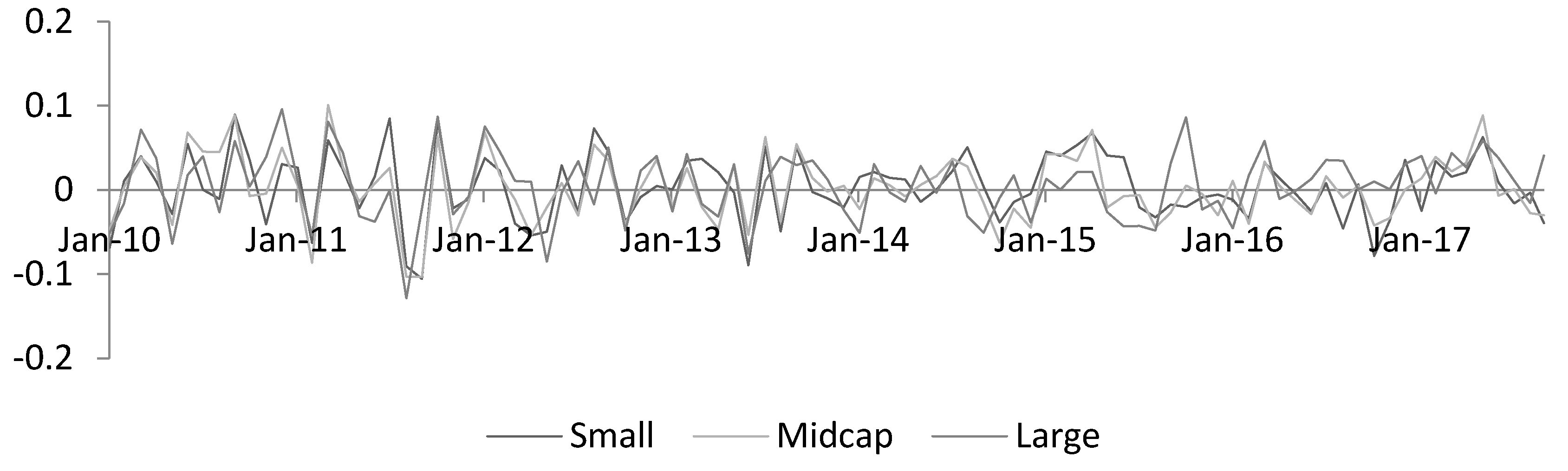
The approach followed in this section was to use indexes to represent both size and style differences. When comparing the returns according to different investment styles the indexes used were the MSCI South Korea Value Index and the MSCI South Korea Growth Index. The monthly returns for all these indexes were obtained for the period from 1997 to 2016 (Figure 2). Similarly, the indexes used to distinguish among the different company sizes were the MSCI South Korea Large Cap Index, the MSCI South Korea Mid Cap Index and the MSCI South Korea Small Cap Index. The monthly returns in all these three indexes can be seen in Figure 3. The time period for the size indexes is shorter due to data availability from the database used (Bloomberg, New York, NY, USA).
3.2. Normality
In order to decide which statistical test to use to compare the performance of the different indexes the first step is to determine if the data follow a normal distribution. The existing academic consensus view is that stock returns do not follow a normal distribution but it is advisable to nevertheless test it for the specific country analyzed. This was done using an Anderson Darling test for the entire time series (Table 1 and Table 2) as well as for the individual years analyzed. The data for the individual years can be seen in the Appendix A (Table A1 and Table A2). The null hypothesis of the test is that stocks returns for these indexes follow a normal distribution. All tests will be done at a five percent significance level. The results when analysing the entire datasets available are mixed. For the style indexes, the test rejects the null hypothesis of a normal distribution but for the size indexes and in all the three cases, the tests fail to reject the null hypothesis. For the majority of the individual years the tests fail to reject the null hypothesis of a normal distribution. There are however some exceptions, such as the 2012 monthly returns of the MSCI South Korea Growth Index or the 2015 monthly returns for the MSCI South Korea Small Cap Index. In these two cases the null hypothesis, at five percent significance, is actually rejected. Given that some of the tests do actually reject the normal hypothesis the approach followed in this article is to use statistical test that do not assume that the returns are normally distributed.
3.3. Size Comparison
The following step is to compare the performance of the different size indexes (small, medium and large companies). This will be done using a Wilcoxon rank sum test. The null hypothesis of this test is that the stock returns come from distributions with the same median. The Wilcoxon test for the entire dataset can be seen in Table 3. The test compared all three pairs of indexes i.e., large cap with mid cap, large cap with small cap and mid cap with small cap. In all three cases the test failed to reject the null hypothesis. The results were identical when comparing the returns of the indexes each year individually (Table 4). All the tests fail to reject the null hypothesis of equal medians. A Kruskal Wallis and a Wilcoxon signed rank test were also used to test the performance of the portfolios (Table 5, Table 6, Table 7 and Table 8). There was remarkable consistency in the results of the tests comparing the performance of stocks in the South Korean market according to company size. As previously mentioned, the available time series for size type indexes is relatively short with full year information only available from 2010 to 2016. It should be mentioned that the obtained p values are rather large. Even at a 10% significance level, all the tests fail to reject that the stocks returns come from a distribution with the same median.
3.4. Style Comparison
The next step was to compare the performance of the value and the growth index in the South Korean stock market. This was done in a similar way as before, using the Wilcoxon test to compare the median of the monthly returns. In this case the indexes used were the previously mentioned value and growth indexes. Once more, the results for both the entire time period (Table 9) as well as when analysing every year (Table 10) independently point towards no significant statistical difference. Similar to the size case the Kruskal Wallis and Wilcoxon signed tests were also used to compare the performance of the portfolios (Table 11, Table 12, Table 13 and Table 14). It should be noted that the style investing indexes have a much longer track record than the size investing indexes. The style indexes allowed for comparison dating back to 1997 when in the case of size indexes comparison were only available for data coming back to 2010. The Wilcoxon tests failed to reject for all the time periods analyzed the hypothesis that the monthly returns of both indexes come from distributions with the same median. There was no apparent exception to this trend for all the comparison at a five percent significance level. Similar to the previous case, the p values obtained are rather large with all tests failing to reject the null hypothesis at both 5% and 10% significances. This also includes the case in which the entire time series is analyzed.
3.5. Methodology—Portfolio Constructed from Individual Stocks
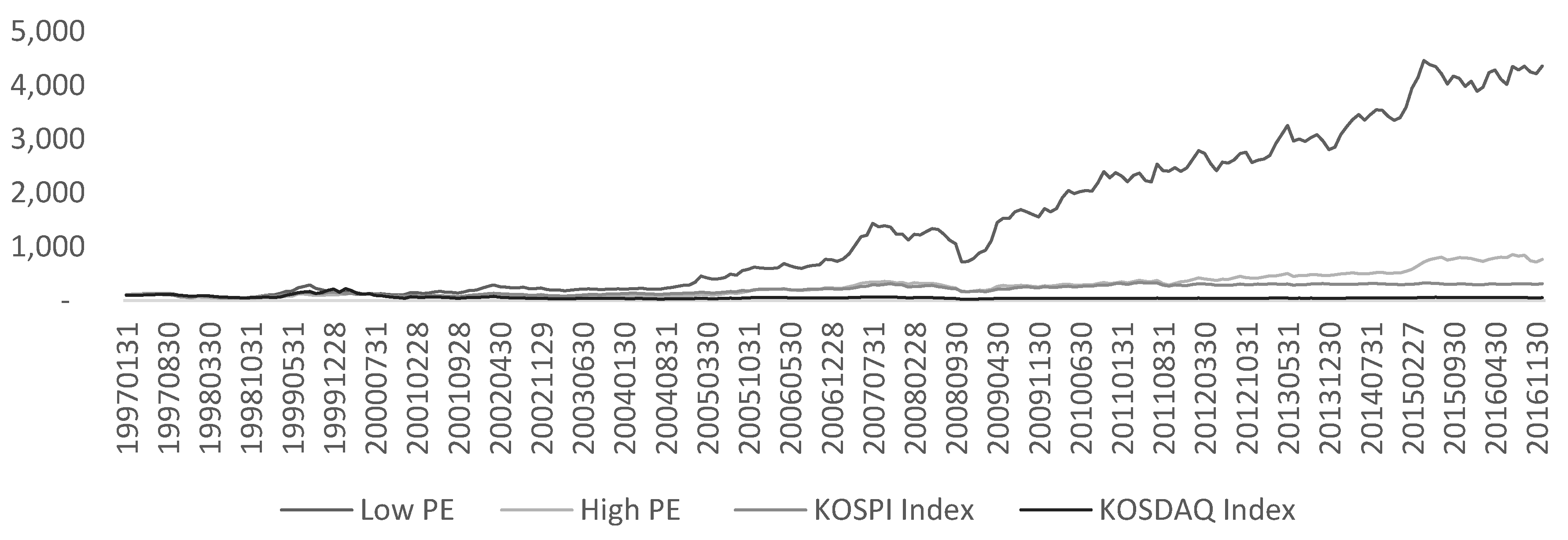
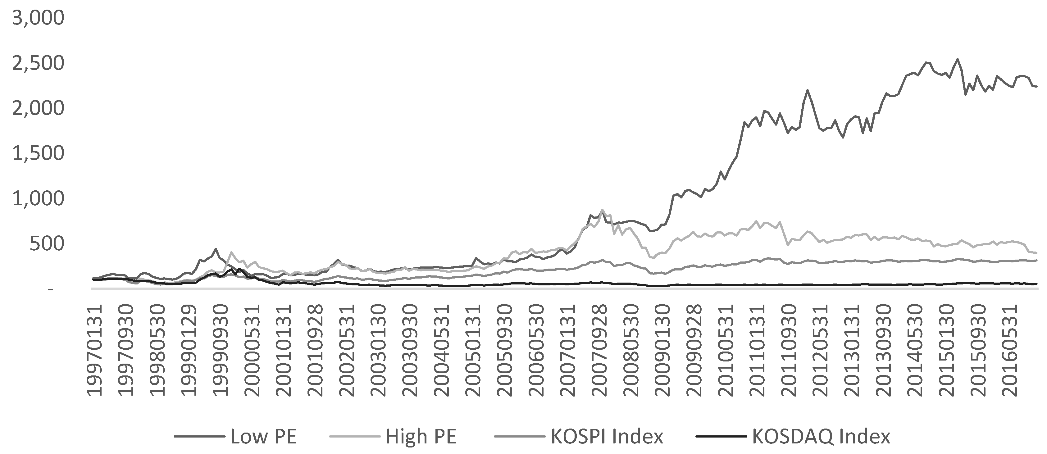
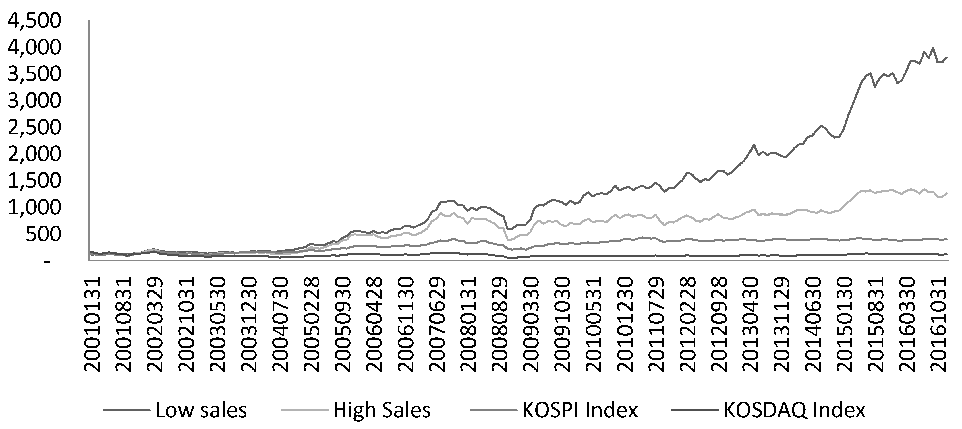
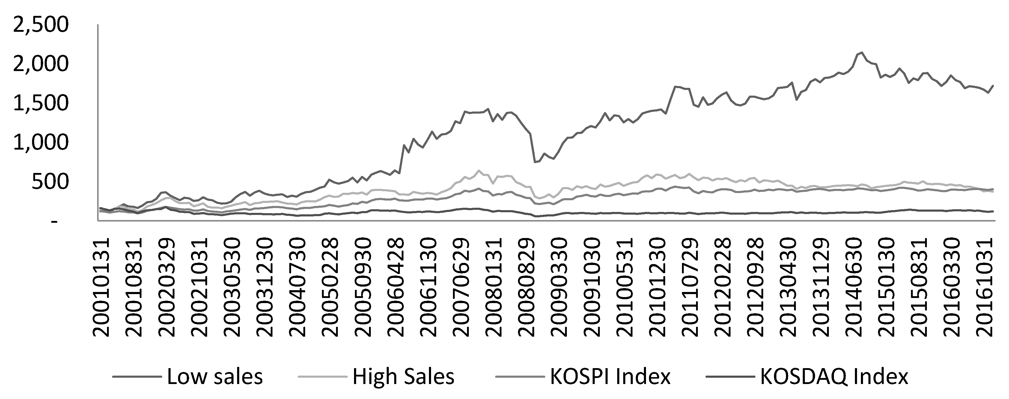
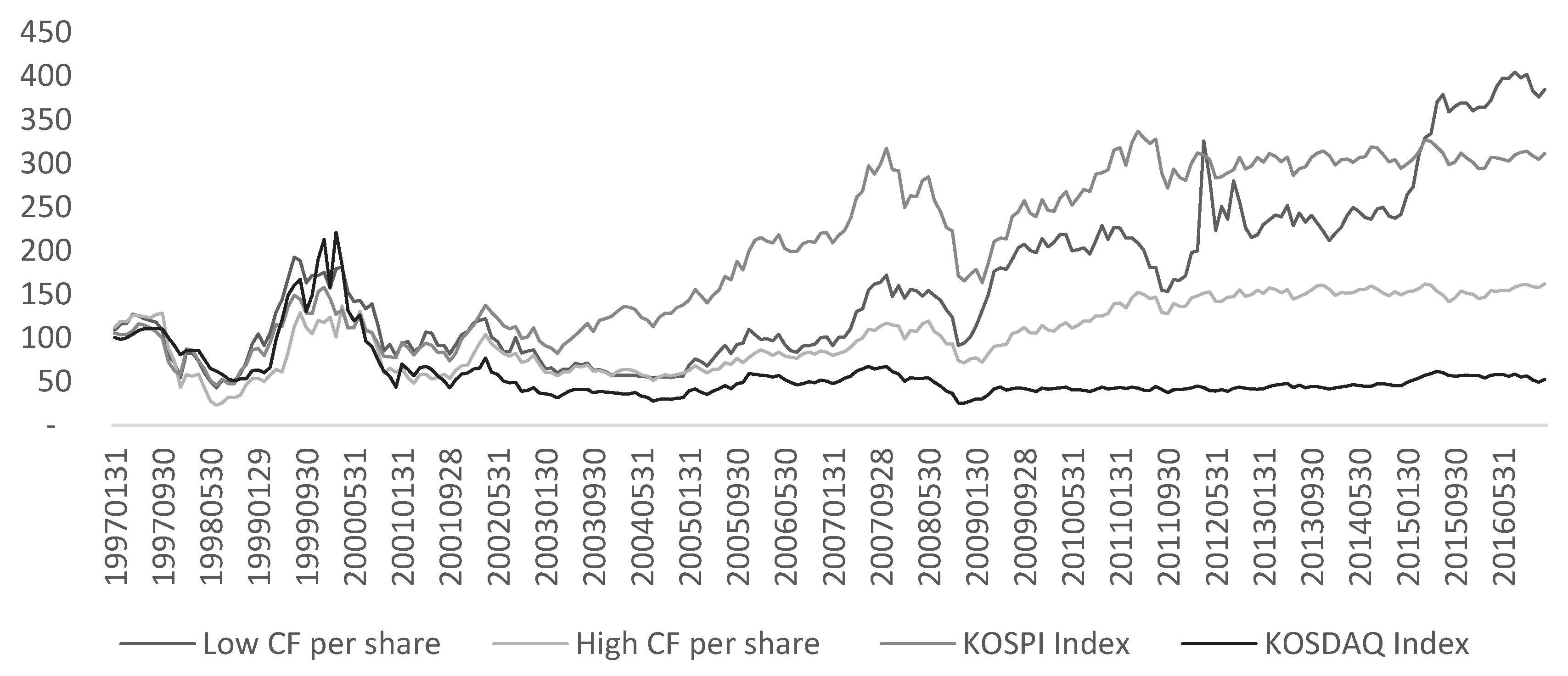
An alternative to using market indexes like the previously mentioned MSCI indexes is to build portfolios from individual stocks using some criteria typically associated with value or growth investment. The first step in creating a portfolio of stocks reflecting value and growth characteristics was obtaining the list of all the stocks listed in Korea. Only stocks listed in the Korea Stock Exchange (KOSPI) or in KOSDAQ, which is a NASDAQ like exchange, were included in the original list of stocks. Stocks listed in the Konex Exchange were explicitly excluded from the analysis as they are typically a smaller, more volatile type of stocks. Only common stocks were included so there in the original list no ETFs, REITS or other listed securities besides common stocks. In the Korean market, there are some listed securities formally classified as common stocks that are called blank check companies. These companies are intended as a venue for future acquisitions and they are not run as traditional companies hence they were excluded from the analysis as well. In a similar approach to (Lakonishok et al. 1994) and (Alfonso Perez 2017c) the portfolios were created using four different metrics P/E, P/B, last 5 years average sales growth and cash flow per share. The data was divided into 10 segments accounting for 10% of the data each. The bottom 10% segment included the companies with then lowest value for each metric, for example P/E. In this way, a portfolio of low (lowest 10% segment) and high (highest 10% segment) were built. The value for each metric was calculated at the end of a given year, for every stock and then used as the constituents of the portfolio in the next year. In this way, it is assumed that the investor does a yearly rebalance of the portfolio. As an example, the 10% of the stocks with the lowest P/E values as of the end of December 2000 will form the portfolio of low P/E stocks for the entire 2001. The stocks selected for a portfolio each year will depend exclusively in those factors. The monthly returns for that portfolio were then calculated. Liquidity considerations were also taken into account and only relatively liquid stocks were included in the portfolios. All the data was obtained from Bloomberg and the period analyzed was from 1997 to 2016. Companies with negative sales growth were not included in the analysis as value investors typically stay away from turnaround situations. The analysis using 5-year average sales growth rate were also shorter, starting in 2001, due to the obvious restriction of needing at least 5 years of sales track record for a large enough sample to build a reasonable portfolio. For each of the four metrics previously mentioned (P/E, P/B, 5-year average sales growth and cash flow per share) two different portfolios were built. One using market capitalization weights and another one using equal weights. The portfolios using market capitalization weight clearly give more importance to large companies. The returns were compared using a Wilcoxon test for the entire period analyzed as well as for each year independently. The results of these tests can be seen in Appendix B (Table A3, Table A4, Table A5 and Table A6). In order to visualize the results a graph showing the value of an initial 100 South Korean Won invested over the mentioned time frame is shown in Figure 4, Figure 5, Figure 6, Figure 7, Figure 8, Figure 9, Figure 10 and Figure 11. It is interesting to see that while for the majority of years and metrics the Wilcoxon test, at a 5% significance level, failed to reject the hypothesis of equal means there appears to be substantial differences in the end values of the portfolios using such metrics. This might be related to the fact that small differences in returns, too small to be detectable by the Wilcoxon test, might compound to large differences in portfolio value after a long period of time.
3.6. Correlation
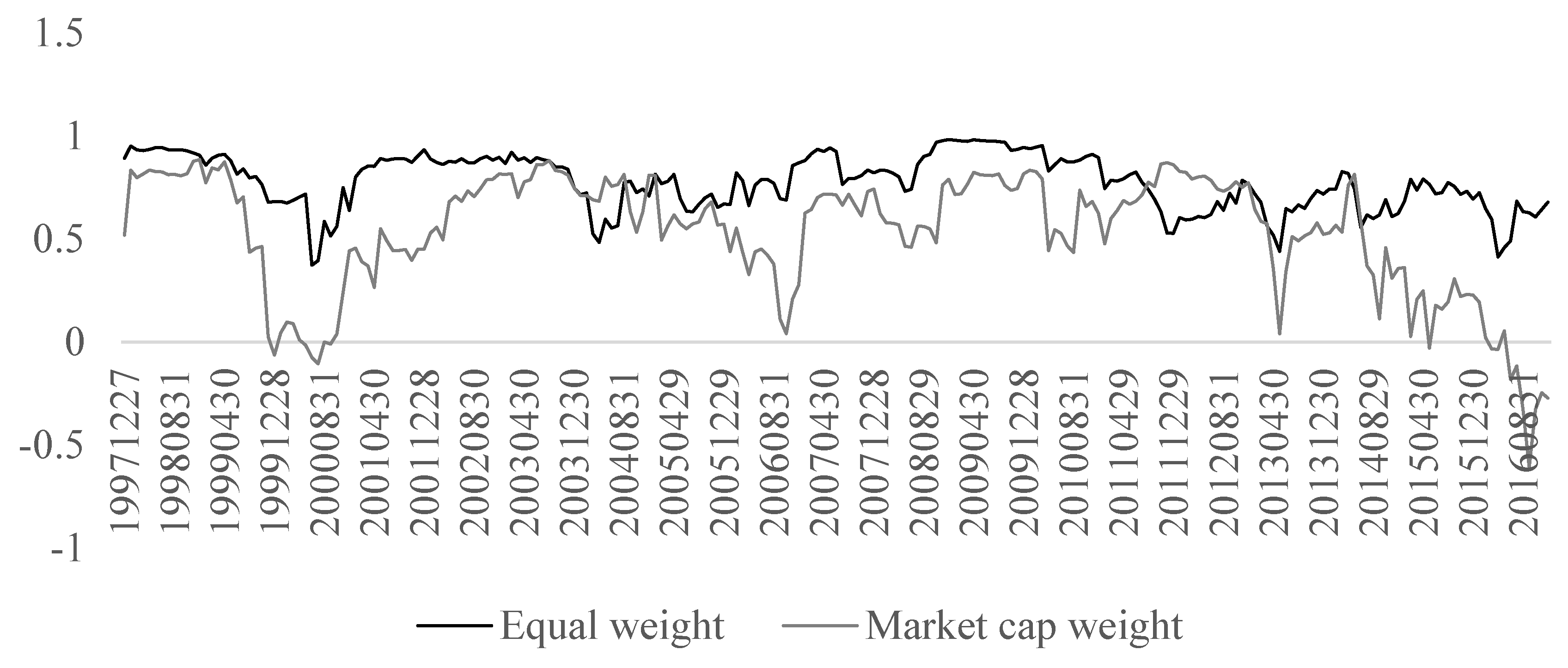
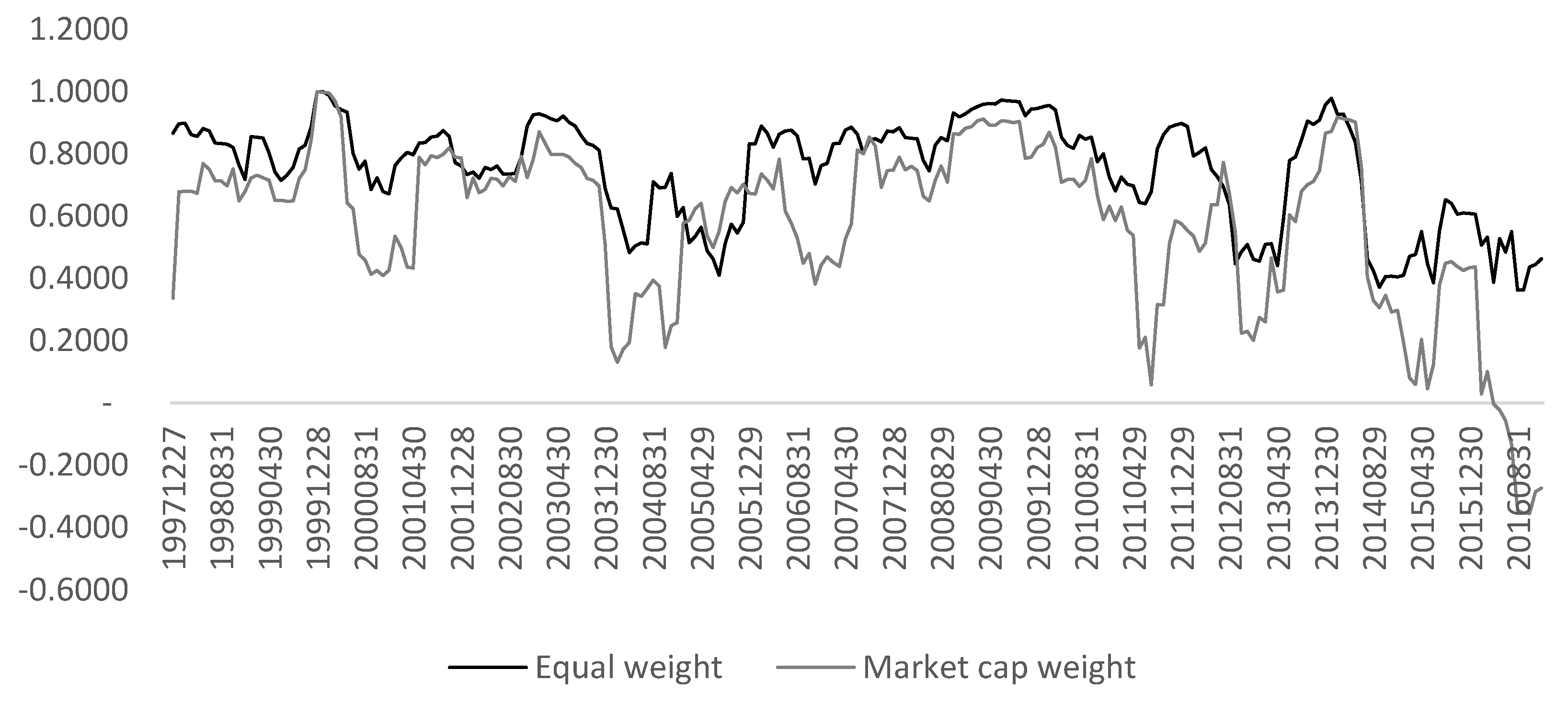
In an attempt to better understand the dynamics of the relationships between the returns of the different portfolios the trailing 12-month correlation for each month was calculated. In this way, each point of the data series is the correlation of the returns in that month and the previous 11 months. This approach was followed for the all four different approaches used i.e., P/E, P/B, last 5-year sales growth and cash flow per share. It will be shown that the correlation value fluctuates substantially over time.
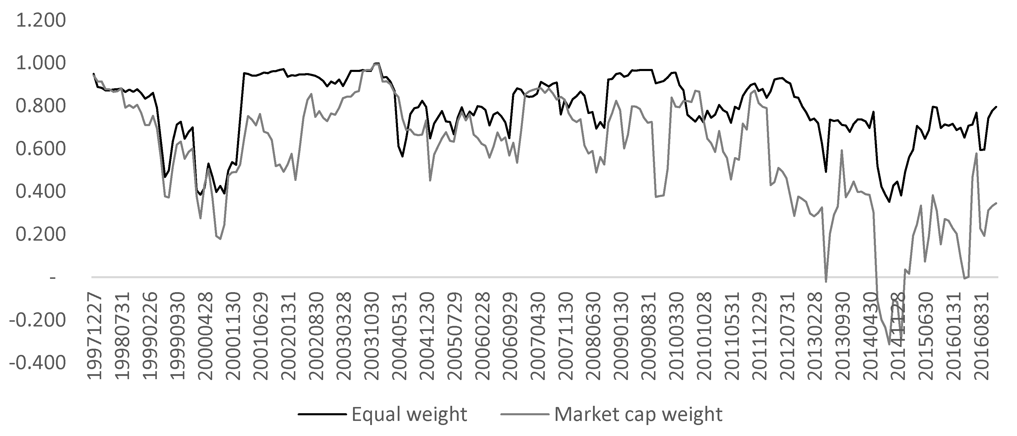
The correlation (12-month trailing) between the returns of the low and high PE portfolios (Figure 12) appears to decrease over time, particularly when the portfolio was built using market capitalization weights. In recent periods the correlation was even negative. It should be noted that historically the correlation has remained positive for most periods. The fluctuations in the value of the correlation seem to be smaller if portfolios are built using an equal weight approach. Similar results are found when using the small P/B and high P/B portfolios (Figure 13) with the point estimate for the value of the correlation decreasing in recent years. The results obtained using cash flow per share (Figure 14) are similar with correlation decreasing over time for the portfolios using the market capitalization approach. In this case negative correlation appears only in a hand full of months. Similar results were obtained when using the 5-year average sales growth metric (Figure 15).
4. Results
The statistical test performed over the monthly returns of the MSCI South Korea Value Index and the MSCI South Korea Growth Index failed to reject, for the majority of the years analyzed, the null hypothesis of coming from distributions with the same median. These tests were performed both using the entire available dataset as well as each year independently. The results obtained were consistent for every year with no statistically significant changes (5% significance) on the results but when the entire time series were analyzed the results were more mixed, particularly for the Kruskal Wallis and Wilcoxon signed rank test perhaps pointing towards some indication of value investing outperforming over very long periods of time, much longer than just a year. It should be noted that even the results for very long time periods are mixed with some of the tests that show contradictory results. A similar approach was followed analysing large, mid and small size companies. The indexes used in this case were the MSCI South Korea Large Cap Index, the MSCI South Korea Mid Cap Index and the MSCI South Korea Small Cap index. The results were once more rather consistent with the formal statistical tests failing to reject the null hypothesis of equal medians. The analysis was done using the entire dataset as well as each year independently with the results remaining the same.
The returns of the portfolios created using low P/E, low P/B, low average sales 5-year growth rate appear to outperform for the period analyzed portfolios created using high P/E, High P/B and high average sales growth rate (Figure 4, Figure 5, Figure 6, Figure 7, Figure 8 and Figure 9) but the Wilcoxon test for the majority of the years indicate that at a 5% significance level there is no statistically significant difference.
It should be noted that there appears to be a substantial difference in the final value of the simulated portfolios. It is interesting that the formal statistical tests do not detect any significant difference in returns for the vast majority of the years despite the substantial differences in final portfolio values. This might be related to small differences in portfolio return (too small to be detected by the test) having a large compound effect over a large period of time. The final values for the portfolios obtained in the simulations are consistently higher when using the equal weight approach compared to market capitalization approach. The results in the simulations using equal weight and low P/E, P/B and average 5-year growth sales were also higher than those obtained by the KOSPI and KOSDAQ indexes. All of the results obtained using these three metrics are consistent with value stocks actually outperforming growth stocks. However, the result using the last metric—cash flow per share—seems to point toward the opposite direction, favouring growth stocks. The point estimates for the portfolios using low cash flow per share were higher than those using high cash flow per share. It should be noted that the point estimates for the market weighted portfolio using low cash flow per share was higher, on a cumulative basis, only in the last couple of years with this portfolio underperforming the KOSPI index in the majority of previous years. It is important to remark once more that the Wilcoxon tests, at a 5% significance, failed to reject the hypothesis of equal means for the majority of years and metrics used. The results for the other two tests were more mixed (see Appendix B).
Correlations between portfolios using high and low value of P/E, P/B, cash flow per share and 5-year average growth sales fluctuate greatly over time, particularly when those portfolios are constructed using market capitalization weights. There seems to be a tendency over the last few years for this correlation to decrease. This tendency appears more clearly, once more, in the portfolios built using market capitalization weight.
5. Discussion
Given that South Korea is a country rather unique in the sense of being not clearly classified as either a developed economy or a developing economy it is not surprising that its stock market has also some peculiarities. The results obtained are mixed but overall point towards the direction of no value or small cap effect in the South Korean Equity market at least when performance is measured on a yearly basis. This result might be a bit counterintuitive as value effect has been detected in the stock markets of many countries and the final value of some of the simulated portfolios with some of the metrics typically associated with value investing appear to be rather different from the results obtained by broad indexes, such as KOSPI and KOSDAQ, as well as when using growth portfolios. Nevertheless, when a rigorous statistical analysis, is used to compare the relative performance of these portfolios then the null hypothesis of equal means of the monthly returns cannot be rejected for the majority of the years analyzed. This might be rather relevant for investors when doing stock allocation decisions and might be even problematic for investors using the Fama-French 5 factor model pointing perhaps to big differences between the stock market of different countries.
The South Korean market seems to have a performance regarding value investment that is rather different from other countries, where value investment appears to consistently outperform. This might be related to the different level of development in the market. The South Korean market is a much younger market than the one in the U.S. or in many other Western countries and perhaps it has not had enough time to mature until a level in which investors follow a disciplined investment approach based on company valuations. The rapid economic development of the country might have also had behavioural implications on investors, who might see that rapid development and thus favour growth stocks rather than companies with more stable cash flows and earnings.
Conflicts of Interest
The author declares no conflict of interest.
Appendix A. Anderson Darling Tests (Per Year)

Table A1.
Value and growth indexes (AD test).
| Year | Value | Growth | ||
|---|---|---|---|---|
| p | H | p | H | |
| 1997 | 0.3745 | 0 | 0.0051 | 1 |
| 1998 | 0.2229 | 0 | 0.3389 | 0 |
| 1999 | 0.3709 | 0 | 0.5461 | 0 |
| 2000 | 0.8889 | 0 | 0.4877 | 0 |
| 2001 | 0.8007 | 0 | 0.4638 | 0 |
| 2002 | 0.3768 | 0 | 0.8080 | 0 |
| 2003 | 0.2874 | 0 | 0.8271 | 0 |
| 2004 | 0.7353 | 0 | 0.8212 | 0 |
| 2005 | 0.5898 | 0 | 0.2760 | 0 |
| 2006 | 0.2354 | 0 | 0.8678 | 0 |
| 2007 | 0.6811 | 0 | 0.8746 | 0 |
| 2008 | 0.2775 | 0 | 0.7535 | 0 |
| 2009 | 0.9098 | 0 | 0.9406 | 0 |
| 2010 | 0.9900 | 0 | 0.5281 | 0 |
| 2011 | 0.3684 | 0 | 0.9711 | 0 |
| 2012 | 0.7510 | 0 | 0.0045 | 1 |
| 2013 | 0.5609 | 0 | 0.4114 | 0 |
| 2014 | 0.8810 | 0 | 0.5310 | 0 |
| 2015 | 0.2424 | 0 | 0.8298 | 0 |
| 2016 | 0.9900 | 0 | 0.5368 | 0 |
Table A2.
Large, mid and small cap indexes (AD test).
| Year | Large | Mid | Small | |||
|---|---|---|---|---|---|---|
| p | H | p | H | p | H | |
| 2010 | 0.8924 | 0 | 0.7416 | 0 | 0.9900 | 0 |
| 2011 | 0.4796 | 0 | 0.6387 | 0 | 0.8053 | 0 |
| 2012 | 0.5468 | 0 | 0.9828 | 0 | 0.5565 | 0 |
| 2013 | 0.1864 | 0 | 0.9378 | 0 | 0.4605 | 0 |
| 2014 | 0.4949 | 0 | 0.8748 | 0 | 0.7604 | 0 |
| 2015 | 0.4709 | 0 | 0.3667 | 0 | 0.0362 | 1 |
| 2016 | 0.6680 | 0 | 0.6439 | 0 | 0.9180 | 0 |
Appendix B
Table A3.
p values for the Wilcoxon Test–Price to Book *.
| Date | EWLPB-HPB | EWLPB-KOSPI | EWLPB-KOSDAQ | EWLPB-MWLPB | EWLPB-MWHPB | EWHPB-KOSPI | EWHPB-KOSDAQ | EWHPB-MWLPB | EWHPB-MWHPB | MWLPB-KOSPI | MWLPB-KOSDAQ | MWHPB-KOSPI | MWHPB-KOSDAQ | MWHPB-MWLPB |
|---|---|---|---|---|---|---|---|---|---|---|---|---|---|---|
| 1997–2016 | 0.225 | 0.209 | 0.033 | 0.557 | 0.220 | 0.931 | 0.751 | 0.885 | 0.980 | 0.528 | 0.133 | 0.972 | 0.392 | 0.492 |
| 1997 | 0.795 | 1.000 | 0.471 | 0.931 | 0.471 | 0.931 | 0.751 | 0.885 | 0.583 | 0.977 | 0.436 | 0.403 | 0.708 | 0.436 |
| 1998 | 0.583 | 0.751 | 0.341 | 0.931 | 0.665 | 0.977 | 0.507 | 0.795 | 0.840 | 0.795 | 0.544 | 0.840 | 0.544 | 0.977 |
| 1999 | 1.000 | 0.931 | 0.371 | 0.471 | 0.471 | 0.931 | 0.371 | 0.471 | 0.471 | 0.708 | 0.260 | 0.708 | 0.260 | 1.000 |
| 2000 | 0.341 | 0.403 | 0.012 | 0.403 | 0.403 | 0.977 | 0.100 | 0.795 | 0.795 | 0.840 | 0.100 | 0.751 | 0.141 | 0.977 |
| 2001 | 0.371 | 0.795 | 0.471 | 0.665 | 0.507 | 0.624 | 1.000 | 0.885 | 1.000 | 0.977 | 0.795 | 0.583 | 0.977 | 0.795 |
| 2002 | 0.840 | 0.840 | 0.583 | 0.931 | 0.708 | 0.885 | 0.665 | 0.708 | 0.708 | 0.840 | 0.471 | 0.751 | 0.436 | 1.000 |
| 2003 | 0.471 | 0.583 | 0.544 | 0.237 | 0.977 | 0.215 | 0.977 | 0.069 | 0.436 | 0.312 | 0.157 | 0.751 | 0.624 | 0.286 |
| 2004 | 0.840 | 0.544 | 0.931 | 0.840 | 0.751 | 0.840 | 0.795 | 0.751 | 0.977 | 0.403 | 0.885 | 0.665 | 0.624 | 0.708 |
| 2005 | 0.312 | 0.371 | 0.583 | 0.931 | 0.371 | 0.840 | 1.000 | 0.544 | 0.708 | 0.507 | 0.665 | 0.751 | 0.624 | 0.403 |
| 2006 | 0.544 | 0.840 | 0.371 | 0.795 | 0.624 | 0.544 | 0.751 | 0.403 | 0.286 | 0.583 | 0.286 | 0.544 | 0.194 | 0.931 |
| 2007 | 0.403 | 0.471 | 0.840 | 0.471 | 0.286 | 0.751 | 0.977 | 0.885 | 0.583 | 0.977 | 0.977 | 0.665 | 0.507 | 0.977 |
| 2008 | 0.751 | 0.795 | 0.583 | 0.977 | 0.977 | 0.931 | 0.795 | 0.708 | 0.665 | 0.840 | 0.708 | 0.840 | 0.708 | 1.000 |
| 2009 | 1.000 | 0.840 | 0.840 | 0.977 | 0.471 | 0.931 | 0.977 | 0.885 | 0.507 | 0.751 | 0.665 | 0.583 | 0.795 | 0.471 |
| 2010 | 0.977 | 0.708 | 0.312 | 0.840 | 0.751 | 0.977 | 0.286 | 0.977 | 0.977 | 1.000 | 0.312 | 0.977 | 0.624 | 0.931 |
| 2011 | 0.840 | 0.583 | 0.977 | 0.403 | 0.931 | 0.751 | 0.931 | 0.583 | 0.751 | 0.583 | 0.544 | 0.977 | 0.977 | 0.840 |
| 2012 | 0.341 | 0.931 | 0.471 | 0.795 | 0.403 | 0.371 | 0.583 | 0.371 | 0.840 | 0.885 | 0.544 | 0.403 | 0.977 | 0.665 |
| 2013 | 0.977 | 0.286 | 0.665 | 0.795 | 0.507 | 0.260 | 0.840 | 0.885 | 0.544 | 0.260 | 0.665 | 1.000 | 0.885 | 0.371 |
| 2014 | 0.624 | 0.126 | 0.471 | 0.885 | 0.665 | 0.312 | 0.708 | 0.708 | 0.931 | 0.126 | 0.507 | 0.436 | 1.000 | 0.507 |
| 2015 | 0.931 | 0.141 | 0.708 | 0.100 | 0.471 | 0.194 | 0.471 | 0.126 | 0.436 | 0.507 | 0.237 | 0.403 | 0.751 | 0.260 |
| 2016 | 0.403 | 0.507 | 0.260 | 0.977 | 0.237 | 0.885 | 0.708 | 0.436 | 0.795 | 0.583 | 0.403 | 0.708 | 0.840 | 0.260 |
* EW and MW stand respectively for equally weighted and market capitalization weighted portfolio.
Table A4.
p values for the Wilcoxon Test–Price to Earnings.
| Date | LPE-HPE | LPE-KOSPI | LPE-KOSDAQ | LPE-MWLPE | LPE-MWHPE | EWHPE-KOSPI | EWHPE-KOSDAQ | EWHPE-MWLPB | EWHPE-MWHPB | MWLPE-KOSPI | MWLPE-KOSDAQ | MWHPE-KOSPI | MWHPE-KOSDAQ | MWHPE-MWLPE |
|---|---|---|---|---|---|---|---|---|---|---|---|---|---|---|
| 1997–2016 | 0.713 | 0.134 | 0.024 | 0.498 | 0.254 | 0.276 | 0.067 | 0.824 | 0.520 | 0.420 | 0.100 | 0.831 | 0.301 | 0.594 |
| 1997 | 0.885 | 0.624 | 1.000 | 0.286 | 0.885 | 0.840 | 0.840 | 0.194 | 0.885 | 0.112 | 0.141 | 0.708 | 0.507 | 0.260 |
| 1998 | 0.840 | 0.751 | 0.312 | 0.840 | 0.840 | 1.000 | 0.751 | 0.583 | 1.000 | 0.840 | 0.471 | 1.000 | 0.751 | 0.583 |
| 1999 | 0.885 | 0.840 | 0.507 | 0.583 | 0.371 | 0.840 | 0.260 | 0.665 | 0.286 | 0.708 | 0.215 | 0.286 | 0.885 | 0.194 |
| 2000 | 0.885 | 0.507 | 0.019 | 0.795 | 0.583 | 0.665 | 0.053 | 0.583 | 0.795 | 0.977 | 0.126 | 0.931 | 0.126 | 0.977 |
| 2001 | 0.471 | 0.795 | 0.624 | 0.665 | 0.583 | 0.708 | 1.000 | 0.708 | 0.977 | 0.931 | 0.583 | 0.665 | 0.931 | 0.840 |
| 2002 | 0.471 | 0.665 | 0.471 | 0.840 | 0.708 | 0.977 | 0.665 | 0.885 | 0.840 | 0.977 | 0.665 | 0.931 | 0.665 | 0.885 |
| 2003 | 0.624 | 0.436 | 0.665 | 0.471 | 0.840 | 0.977 | 0.371 | 0.977 | 0.840 | 0.708 | 0.436 | 0.931 | 0.840 | 0.885 |
| 2004 | 0.507 | 0.471 | 0.100 | 0.194 | 0.175 | 0.977 | 0.471 | 0.795 | 0.751 | 0.795 | 0.665 | 0.665 | 0.795 | 0.977 |
| 2005 | 0.840 | 0.795 | 0.931 | 0.194 | 0.840 | 0.194 | 0.471 | 0.157 | 0.708 | 0.286 | 0.286 | 0.583 | 0.840 | 0.157 |
| 2006 | 0.931 | 0.665 | 0.237 | 0.403 | 0.977 | 0.751 | 0.237 | 0.371 | 0.977 | 0.078 | 0.061 | 0.665 | 0.237 | 0.194 |
| 2007 | 0.931 | 0.751 | 0.544 | 0.795 | 0.795 | 0.840 | 0.583 | 0.583 | 0.507 | 0.544 | 0.436 | 0.436 | 0.260 | 0.977 |
| 2008 | 0.751 | 0.665 | 0.471 | 0.885 | 0.544 | 0.885 | 0.665 | 0.312 | 0.885 | 0.436 | 0.286 | 0.795 | 0.977 | 0.341 |
| 2009 | 0.507 | 0.507 | 0.471 | 0.544 | 0.624 | 0.840 | 0.931 | 0.931 | 0.795 | 0.931 | 0.977 | 0.751 | 0.840 | 1.000 |
| 2010 | 0.471 | 0.544 | 0.215 | 0.403 | 0.403 | 1.000 | 0.436 | 0.175 | 0.708 | 0.194 | 0.053 | 0.751 | 0.795 | 0.157 |
| 2011 | 0.471 | 0.708 | 0.840 | 0.795 | 0.840 | 0.544 | 0.624 | 0.544 | 0.885 | 0.840 | 0.931 | 1.000 | 0.751 | 1.000 |
| 2012 | 0.583 | 0.977 | 0.751 | 0.795 | 0.977 | 0.977 | 0.708 | 0.507 | 0.795 | 0.624 | 0.931 | 0.931 | 0.751 | 0.840 |
| 2013 | 0.977 | 0.583 | 0.977 | 0.795 | 0.583 | 0.237 | 0.583 | 0.840 | 0.795 | 0.471 | 0.665 | 0.931 | 0.751 | 0.471 |
| 2014 | 0.436 | 0.112 | 0.583 | 0.624 | 0.089 | 0.194 | 1.000 | 0.885 | 0.157 | 0.260 | 0.751 | 0.341 | 0.141 | 0.126 |
| 2015 | 0.286 | 0.507 | 0.795 | 0.403 | 0.665 | 0.030 | 0.341 | 0.100 | 0.069 | 0.795 | 0.341 | 0.885 | 0.471 | 0.885 |
| 2016 | 0.977 | 0.885 | 0.583 | 0.885 | 0.341 | 0.885 | 0.583 | 1.000 | 0.544 | 0.341 | 0.931 | 0.215 | 0.885 | 0.312 |
Table A5.
p values for the Wilcoxon Test–Cash flow per share.
| Date | LCF-HCF | LCF-KOSPI | LCF-KOSDAQ | LCF-MWLCF | LCF-MWHCF | EWHCF-KOSPI | EWHCF-KOSDAQ | EWHCF-MWLCF | EWHCF-MWHCF | MWLCF-KOSPI | MWLCF-KOSDAQ | MWHCF-KOSPI | MWHCF-KOSDAQ | MWHCF-MWLCF |
|---|---|---|---|---|---|---|---|---|---|---|---|---|---|---|
| 1997–2016 | 0.980 | 0.245 | 0.044 | 0.414 | 0.358 | 0.196 | 0.041 | 0.358 | 0.320 | 0.788 | 0.308 | 0.759 | 0.265 | 0.979 |
| 1997 | 0.507 | 0.624 | 0.795 | 0.795 | 1.000 | 0.286 | 0.312 | 0.312 | 0.507 | 0.931 | 0.624 | 0.471 | 0.977 | 0.544 |
| 1998 | 0.977 | 0.795 | 0.471 | 0.977 | 0.931 | 0.885 | 0.157 | 0.977 | 0.977 | 0.931 | 0.583 | 1.000 | 0.312 | 0.977 |
| 1999 | 0.708 | 0.507 | 0.237 | 0.665 | 0.665 | 0.403 | 0.215 | 0.436 | 0.436 | 0.931 | 0.436 | 0.977 | 0.507 | 0.931 |
| 2000 | 0.665 | 0.403 | 0.035 | 0.436 | 0.583 | 0.931 | 0.078 | 1.000 | 0.931 | 1.000 | 0.157 | 0.840 | 0.286 | 0.931 |
| 2001 | 0.931 | 0.840 | 0.840 | 0.665 | 0.977 | 0.708 | 1.000 | 0.665 | 0.977 | 0.885 | 0.840 | 0.665 | 0.931 | 0.885 |
| 2002 | 0.665 | 0.795 | 0.665 | 0.708 | 0.665 | 0.885 | 0.403 | 0.507 | 1.000 | 0.544 | 0.931 | 0.885 | 0.403 | 0.507 |
| 2003 | 0.885 | 0.583 | 0.665 | 0.341 | 0.403 | 0.665 | 0.665 | 0.286 | 0.371 | 0.157 | 0.583 | 0.194 | 0.665 | 0.931 |
| 2004 | 0.126 | 0.751 | 0.885 | 0.624 | 0.885 | 0.215 | 0.089 | 0.017 | 0.157 | 0.371 | 0.931 | 0.751 | 0.624 | 0.624 |
| 2005 | 0.260 | 0.194 | 0.583 | 0.507 | 0.100 | 0.885 | 0.885 | 0.665 | 0.544 | 0.544 | 0.885 | 0.624 | 0.665 | 0.260 |
| 2006 | 0.341 | 0.708 | 0.583 | 0.795 | 0.977 | 0.751 | 0.215 | 0.583 | 0.403 | 0.885 | 0.583 | 0.708 | 0.544 | 0.977 |
| 2007 | 0.751 | 0.795 | 0.544 | 0.665 | 0.708 | 0.507 | 0.286 | 0.931 | 0.507 | 0.583 | 0.312 | 0.977 | 0.583 | 0.436 |
| 2008 | 0.977 | 0.840 | 0.624 | 0.840 | 0.931 | 0.840 | 0.624 | 0.931 | 0.977 | 0.977 | 0.665 | 0.751 | 0.624 | 1.000 |
| 2009 | 0.624 | 0.708 | 0.665 | 0.665 | 0.624 | 0.840 | 0.931 | 0.260 | 0.931 | 0.403 | 0.371 | 0.931 | 0.977 | 0.341 |
| 2010 | 0.583 | 0.885 | 0.544 | 0.840 | 1.000 | 0.624 | 0.215 | 0.471 | 0.708 | 0.795 | 0.840 | 0.977 | 0.312 | 0.751 |
| 2011 | 0.708 | 0.436 | 0.708 | 0.260 | 0.624 | 0.708 | 0.931 | 0.436 | 0.977 | 0.795 | 0.507 | 0.665 | 1.000 | 0.403 |
| 2012 | 0.885 | 1.000 | 0.471 | 0.665 | 0.931 | 0.931 | 0.624 | 0.583 | 0.751 | 0.583 | 0.665 | 0.885 | 0.544 | 0.544 |
| 2013 | 0.885 | 0.751 | 0.840 | 0.751 | 0.624 | 0.371 | 0.795 | 0.583 | 0.371 | 0.931 | 0.708 | 0.931 | 0.885 | 0.931 |
| 2014 | 0.403 | 0.030 | 0.260 | 0.624 | 0.078 | 0.126 | 0.544 | 0.885 | 0.194 | 0.215 | 0.708 | 0.751 | 0.403 | 0.237 |
| 2015 | 0.089 | 0.023 | 0.260 | 0.708 | 0.023 | 0.544 | 0.507 | 0.341 | 0.436 | 0.175 | 0.583 | 1.000 | 0.215 | 0.141 |
| 2016 | 0.544 | 0.371 | 0.371 | 0.544 | 0.507 | 0.977 | 0.751 | 0.751 | 0.624 | 0.544 | 0.708 | 0.507 | 0.665 | 0.931 |
Table A6.
p values for the Wilcoxon Test–Average last 5 years growth rate.
| Date | L-HSales | LSales-KOSPI | LSales-KOSDAQ | LSales-MWLSales | LSales-MWHSales | EWHSales-KOSPI | EWHSales-KOSDAQ | EWHSales-MWLSales | EWHSales-MWHSales | MWLSales-KOSPI | MWLSales-KOSDAQ | MWHSales-KOSPI | MWHSales-KOSDAQ | MWHSales-MWLSale |
|---|---|---|---|---|---|---|---|---|---|---|---|---|---|---|
| 2001–2016 | 0.931 | 0.840 | 0.583 | 0.665 | 0.708 | 0.583 | 0.403 | 0.403 | 0.795 | 0.708 | 0.977 | 0.371 | 0.194 | 0.312 |
| 2001 | 0.840 | 0.708 | 0.583 | 0.286 | 0.708 | 0.977 | 0.795 | 0.436 | 0.840 | 0.371 | 0.260 | 0.665 | 0.665 | 0.751 |
| 2002 | 0.795 | 1.000 | 0.471 | 0.931 | 0.795 | 0.885 | 0.544 | 0.840 | 0.708 | 0.840 | 0.436 | 0.471 | 0.286 | 0.885 |
| 2003 | 0.708 | 0.312 | 0.544 | 0.260 | 0.260 | 0.175 | 0.371 | 0.237 | 0.260 | 0.751 | 0.708 | 0.795 | 0.665 | 1.000 |
| 2004 | 0.708 | 0.341 | 0.112 | 0.840 | 0.175 | 0.931 | 0.436 | 0.885 | 0.795 | 0.544 | 0.341 | 0.977 | 0.665 | 0.507 |
| 2005 | 0.708 | 0.312 | 0.544 | 0.260 | 0.260 | 0.175 | 0.371 | 0.237 | 0.260 | 0.751 | 0.708 | 0.795 | 0.665 | 1.000 |
| 2006 | 0.708 | 0.885 | 0.312 | 1.000 | 0.312 | 0.795 | 0.583 | 0.885 | 0.795 | 0.931 | 0.583 | 0.157 | 0.751 | 0.840 |
| 2007 | 0.931 | 0.840 | 0.583 | 0.665 | 0.708 | 0.583 | 0.403 | 0.403 | 0.795 | 0.708 | 0.977 | 0.371 | 0.194 | 0.312 |
| 2008 | 0.885 | 0.931 | 0.507 | 0.885 | 0.544 | 0.977 | 0.665 | 1.000 | 0.795 | 0.840 | 0.583 | 0.885 | 0.931 | 0.665 |
| 2009 | 0.931 | 0.977 | 0.977 | 1.000 | 0.795 | 0.885 | 0.931 | 0.931 | 0.931 | 1.000 | 0.977 | 0.977 | 0.977 | 0.885 |
| 2010 | 0.977 | 0.977 | 0.371 | 0.840 | 0.751 | 0.885 | 0.544 | 0.840 | 0.885 | 0.708 | 0.708 | 0.665 | 0.286 | 0.403 |
| 2011 | 0.708 | 0.583 | 0.665 | 0.840 | 0.583 | 0.885 | 0.931 | 0.751 | 0.840 | 0.624 | 0.931 | 0.840 | 0.885 | 0.436 |
| 2012 | 0.751 | 0.885 | 0.544 | 0.624 | 0.624 | 0.751 | 0.885 | 0.795 | 0.977 | 0.751 | 0.708 | 0.840 | 0.931 | 0.977 |
| 2013 | 0.708 | 0.286 | 0.403 | 0.931 | 0.175 | 0.237 | 0.708 | 1.000 | 0.215 | 0.286 | 0.665 | 0.260 | 0.371 | 0.078 |
| 2014 | 0.544 | 0.100 | 0.312 | 0.341 | 0.312 | 0.341 | 0.885 | 0.708 | 0.795 | 0.583 | 0.840 | 0.371 | 0.931 | 0.977 |
| 2015 | 0.583 | 0.026 | 0.237 | 0.030 | 0.061 | 0.126 | 0.583 | 0.078 | 0.175 | 0.977 | 0.175 | 0.840 | 0.544 | 0.665 |
| 2016 | 0.624 | 0.624 | 0.583 | 0.403 | 0.126 | 0.544 | 0.751 | 0.977 | 0.341 | 0.403 | 0.931 | 0.112 | 0.544 | 0.341 |
Table A7.
p values for the Kruskal Wallis Test–Price to Book.
| Date | EWLPB-HPB | EWLPB-KOSPI | EWLPB-KOSDAQ | EWLPB-MWLPB | EWLPB-MWHPB | EWHPB-KOSPI | EWHPB-KOSDAQ | EWHPB-MWLPB | EWHPB-MWHPB | MWLPB-KOSPI | MWLPB-KOSDAQ | MWHPB-KOSPI | MWHPB-KOSDAQ | MWHPB-MWLPB |
|---|---|---|---|---|---|---|---|---|---|---|---|---|---|---|
| 1997–2016 | 0.224 | 0.209 | 0.033 | 0.556 | 0.220 | 0.209 | 0.031 | 0.461 | 0.980 | 0.530 | 0.133 | 0.972 | 0.392 | 0.492 |
| 1997 | 0.773 | 1.000 | 0.453 | 0.908 | 0.453 | 0.908 | 0.729 | 0.863 | 0.564 | 0.954 | 0.419 | 0.954 | 0.686 | 0.908 |
| 1998 | 0.564 | 0.729 | 0.326 | 0.908 | 0.644 | 0.905 | 0.488 | 0.773 | 0.817 | 0.773 | 0.525 | 0.773 | 0.525 | 1.000 |
| 1999 | 1.000 | 0.908 | 0.356 | 0.453 | 0.453 | 0.908 | 0.356 | 0.453 | 0.453 | 0.686 | 0.248 | 0.686 | 0.248 | 0.908 |
| 2000 | 0.326 | 0.387 | 0.011 | 0.387 | 0.387 | 0.905 | 0.094 | 0.773 | 0.773 | 0.817 | 0.094 | 0.817 | 0.133 | 1.000 |
| 2001 | 0.356 | 0.773 | 0.453 | 0.644 | 0.488 | 0.603 | 1.000 | 0.863 | 1.000 | 0.954 | 0.773 | 0.954 | 0.954 | 0.863 |
| 2002 | 0.817 | 0.817 | 0.564 | 0.908 | 0.686 | 0.863 | 0.644 | 0.686 | 0.686 | 0.817 | 0.453 | 0.817 | 0.419 | 0.908 |
| 2003 | 0.453 | 0.564 | 0.525 | 0.225 | 0.954 | 0.204 | 0.954 | 0.065 | 0.419 | 0.299 | 0.149 | 0.299 | 0.603 | 0.908 |
| 2004 | 0.817 | 0.525 | 0.908 | 0.817 | 0.729 | 0.817 | 0.773 | 0.729 | 0.954 | 0.387 | 0.863 | 0.387 | 0.603 | 0.908 |
| 2005 | 0.299 | 0.356 | 0.564 | 0.908 | 0.356 | 0.817 | 1.000 | 0.525 | 0.686 | 0.488 | 0.644 | 0.488 | 0.603 | 1.000 |
| 2006 | 0.525 | 0.817 | 0.356 | 0.773 | 0.603 | 0.525 | 0.729 | 0.387 | 0.273 | 0.564 | 0.273 | 0.564 | 0.184 | 0.863 |
| 2007 | 0.003 | 0.003 | 0.003 | 0.003 | 0.004 | 0.729 | 0.863 | 0.863 | 0.564 | 0.954 | 0.954 | 0.954 | 0.488 | 1.000 |
| 2008 | 0.729 | 0.773 | 0.564 | 0.954 | 0.954 | 0.908 | 0.773 | 0.686 | 0.644 | 0.817 | 0.686 | 0.817 | 0.686 | 0.908 |
| 2009 | 1.000 | 0.817 | 0.817 | 0.954 | 0.453 | 0.908 | 0.954 | 0.863 | 0.488 | 0.729 | 0.644 | 0.729 | 0.773 | 1.000 |
| 2010 | 0.954 | 0.686 | 0.299 | 0.817 | 0.729 | 0.954 | 0.273 | 0.954 | 0.954 | 1.000 | 0.299 | 1.000 | 0.603 | 0.863 |
| 2011 | 0.817 | 0.564 | 0.954 | 0.387 | 0.908 | 0.729 | 0.908 | 0.564 | 0.729 | 0.564 | 0.525 | 0.564 | 0.954 | 0.908 |
| 2012 | 0.326 | 0.908 | 0.453 | 0.773 | 0.387 | 0.356 | 0.564 | 0.356 | 0.817 | 0.863 | 0.525 | 0.863 | 0.954 | 0.863 |
| 2013 | 0.954 | 0.273 | 0.644 | 0.773 | 0.488 | 0.248 | 0.817 | 0.863 | 0.525 | 0.248 | 0.644 | 0.248 | 0.863 | 1.000 |
| 2014 | 0.603 | 0.119 | 0.453 | 0.863 | 0.644 | 0.299 | 0.686 | 0.686 | 0.908 | 0.119 | 0.488 | 0.119 | 1.000 | 0.908 |
| 2015 | 0.908 | 0.133 | 0.686 | 0.094 | 0.453 | 0.184 | 0.453 | 0.119 | 0.419 | 0.488 | 0.225 | 0.488 | 0.729 | 0.863 |
| 2016 | 0.387 | 0.488 | 0.248 | 0.954 | 0.225 | 0.863 | 0.686 | 0.419 | 0.773 | 0.564 | 0.387 | 0.564 | 0.817 | 1.000 |
Table A8.
p values for the Kruskal Wallis Test–Price to earnings.
| Date | LPE-HPE | LPE-KOSPI | LPE-KOSDAQ | LPE-MWLPE | LPE-MWHPE | EWHPE-KOSPI | EWHPE-KOSDAQ | EWHPE-MWLPB | EWHPE-MWHPB | MWLPE-KOSPI | MWLPE-KOSDAQ | MWHPE-KOSPI | MWHPE-KOSDAQ | MWHPE-MWLPE |
|---|---|---|---|---|---|---|---|---|---|---|---|---|---|---|
| 1997–2016 | 0.713 | 0.134 | 0.024 | 0.498 | 0.254 | 0.134 | 0.024 | 0.498 | 0.498 | 0.411 | 0.097 | 0.419 | 0.100 | 0.594 |
| 1997 | 1.000 | 0.603 | 1.000 | 0.273 | 0.863 | 0.603 | 1.000 | 0.273 | 0.863 | 0.106 | 0.133 | 0.686 | 0.488 | 0.248 |
| 1998 | 0.823 | 0.729 | 0.298 | 0.817 | 0.817 | 0.729 | 0.299 | 0.817 | 0.817 | 0.817 | 0.453 | 1.000 | 0.729 | 0.564 |
| 1999 | 0.957 | 0.817 | 0.488 | 0.564 | 0.356 | 0.817 | 0.488 | 0.564 | 0.356 | 0.686 | 0.204 | 0.273 | 0.863 | 0.184 |
| 2000 | 0.957 | 0.488 | 0.018 | 0.773 | 0.564 | 0.488 | 0.018 | 0.773 | 0.564 | 0.954 | 0.119 | 0.908 | 0.119 | 0.954 |
| 2001 | 1.000 | 0.773 | 0.603 | 0.644 | 0.564 | 0.773 | 0.603 | 0.644 | 0.564 | 0.733 | 0.564 | 0.644 | 0.908 | 0.817 |
| 2002 | 0.823 | 0.644 | 0.453 | 0.817 | 0.686 | 0.644 | 0.453 | 0.817 | 0.686 | 0.908 | 0.644 | 0.908 | 0.644 | 0.863 |
| 2003 | 0.957 | 0.419 | 0.644 | 0.453 | 0.000 | 0.419 | 0.644 | 0.453 | 0.000 | 0.954 | 0.419 | 0.000 | 0.000 | 0.000 |
| 2004 | 1.000 | 0.453 | 0.094 | 0.184 | 0.166 | 0.453 | 0.094 | 0.184 | 0.166 | 0.686 | 0.644 | 0.644 | 0.773 | 0.954 |
| 2005 | 1.000 | 0.773 | 0.908 | 0.184 | 0.817 | 0.773 | 0.908 | 0.184 | 0.817 | 0.773 | 0.273 | 0.564 | 0.817 | 0.149 |
| 2006 | 0.823 | 0.644 | 0.225 | 0.387 | 0.954 | 0.644 | 0.225 | 0.387 | 0.954 | 0.273 | 0.057 | 0.644 | 0.225 | 0.184 |
| 2007 | 0.732 | 0.729 | 0.525 | 0.773 | 0.773 | 0.729 | 0.525 | 0.773 | 0.773 | 0.074 | 0.419 | 0.419 | 0.248 | 0.954 |
| 2008 | 0.732 | 0.644 | 0.453 | 0.863 | 0.525 | 0.644 | 0.453 | 0.863 | 0.525 | 0.525 | 0.273 | 0.773 | 0.954 | 0.326 |
| 2009 | 0.898 | 0.488 | 0.453 | 0.525 | 0.603 | 0.488 | 0.453 | 0.525 | 0.603 | 0.419 | 0.954 | 0.729 | 0.817 | 1.000 |
| 2010 | 1.000 | 0.525 | 0.204 | 0.387 | 0.387 | 0.525 | 0.204 | 0.387 | 0.387 | 0.908 | 0.050 | 0.729 | 0.773 | 0.149 |
| 2011 | 0.957 | 0.686 | 0.817 | 0.773 | 0.817 | 0.686 | 0.817 | 0.773 | 0.817 | 0.184 | 0.908 | 1.000 | 0.729 | 1.000 |
| 2012 | 0.898 | 0.954 | 0.729 | 0.773 | 0.954 | 0.954 | 0.729 | 0.773 | 0.954 | 0.817 | 0.908 | 0.908 | 0.729 | 0.817 |
| 2013 | 0.898 | 0.564 | 0.954 | 0.773 | 0.564 | 0.564 | 0.954 | 0.773 | 0.564 | 0.603 | 0.644 | 0.908 | 0.729 | 0.453 |
| 2014 | 0.767 | 0.106 | 0.564 | 0.603 | 0.083 | 0.106 | 0.564 | 0.603 | 0.083 | 0.453 | 0.729 | 0.326 | 0.133 | 0.119 |
| 2015 | 0.767 | 0.488 | 0.773 | 0.387 | 0.644 | 0.488 | 0.773 | 0.387 | 0.644 | 0.773 | 0.326 | 0.863 | 0.453 | 0.863 |
| 2016 | 1.000 | 0.863 | 0.564 | 0.863 | 0.326 | 0.863 | 0.564 | 0.863 | 0.326 | 0.326 | 0.908 | 0.204 | 0.863 | 0.299 |
Table A9.
p values for the Kruskal Wallis Test–Cash flow per share.
| Date | LCF-HCF | LCF-KOSPI | LCF-KOSDAQ | LCF-MWLCF | LCF-MWHCF | EWHCF-KOSPI | EWHCF-KOSDAQ | EWHCF-MWLCF | EWHCF-MWHCF | MWLCF-KOSPI | MWLCF-KOSDAQ | MWHCF-KOSPI | MWHCF-KOSDAQ | MWHCF-MWLCF |
|---|---|---|---|---|---|---|---|---|---|---|---|---|---|---|
| 1997–2016 | 0.980 | 0.245 | 0.044 | 0.413 | 0.358 | 0.245 | 0.044 | 0.413 | 0.358 | 0.788 | 0.308 | 0.759 | 0.264 | 0.979 |
| 1997 | 0.488 | 0.603 | 0.773 | 0.773 | 1.000 | 0.603 | 0.603 | 0.773 | 1.000 | 0.603 | 0.773 | 0.603 | 0.773 | 0.773 |
| 1998 | 0.954 | 0.773 | 0.453 | 0.954 | 0.908 | 0.773 | 0.564 | 0.954 | 0.908 | 0.773 | 0.453 | 0.773 | 0.453 | 0.954 |
| 1999 | 0.033 | 0.488 | 0.225 | 0.644 | 0.644 | 0.488 | 0.419 | 0.644 | 0.644 | 0.488 | 0.225 | 0.488 | 0.225 | 0.644 |
| 2000 | 0.644 | 0.387 | 0.817 | 0.419 | 0.564 | 0.387 | 0.149 | 0.419 | 0.564 | 0.387 | 0.033 | 0.387 | 0.033 | 0.419 |
| 2001 | 0.908 | 0.817 | 0.644 | 0.644 | 0.954 | 0.817 | 0.817 | 0.644 | 0.954 | 0.814 | 0.817 | 0.817 | 0.817 | 0.644 |
| 2002 | 0.644 | 0.773 | 0.644 | 0.686 | 0.644 | 0.773 | 0.908 | 0.686 | 0.644 | 0.773 | 0.644 | 0.773 | 0.644 | 0.686 |
| 2003 | 0.863 | 0.564 | 0.863 | 0.326 | 0.387 | 0.564 | 0.564 | 0.326 | 0.387 | 0.564 | 0.863 | 0.564 | 0.644 | 0.326 |
| 2004 | 0.119 | 0.729 | 0.564 | 0.603 | 0.863 | 0.729 | 0.908 | 0.603 | 0.863 | 0.729 | 0.564 | 0.729 | 0.863 | 0.603 |
| 2005 | 0.248 | 0.184 | 0.564 | 0.488 | 0.094 | 0.184 | 0.863 | 0.488 | 0.094 | 0.184 | 0.564 | 0.184 | 0.564 | 0.488 |
| 2006 | 0.326 | 0.686 | 0.525 | 0.773 | 0.954 | 0.686 | 0.564 | 0.773 | 0.954 | 0.686 | 0.525 | 0.686 | 0.564 | 0.773 |
| 2007 | 0.729 | 0.773 | 0.603 | 0.644 | 0.686 | 0.773 | 0.299 | 0.644 | 0.686 | 0.773 | 0.603 | 0.773 | 0.525 | 0.644 |
| 2008 | 0.954 | 0.817 | 0.644 | 0.817 | 0.908 | 0.817 | 0.644 | 0.817 | 0.908 | 0.817 | 0.644 | 0.817 | 0.603 | 0.817 |
| 2009 | 0.603 | 0.686 | 0.525 | 0.644 | 0.603 | 0.686 | 0.356 | 0.644 | 0.603 | 0.686 | 0.525 | 0.686 | 0.644 | 0.644 |
| 2010 | 0.564 | 0.863 | 0.686 | 0.817 | 1.000 | 0.863 | 0.817 | 0.817 | 1.000 | 0.863 | 0.686 | 0.863 | 0.686 | 0.817 |
| 2011 | 0.686 | 0.419 | 0.453 | 0.248 | 0.603 | 0.419 | 0.488 | 0.248 | 0.603 | 0.419 | 0.453 | 0.419 | 0.453 | 0.248 |
| 2012 | 0.863 | 1.000 | 0.817 | 0.644 | 0.908 | 1.000 | 0.644 | 0.644 | 0.908 | 1.000 | 0.817 | 1.000 | 0.817 | 0.644 |
| 2013 | 0.387 | 0.729 | 0.248 | 0.729 | 0.603 | 0.729 | 0.686 | 0.729 | 0.603 | 0.729 | 0.248 | 0.729 | 0.248 | 0.729 |
| 2014 | 0.635 | 0.028 | 0.248 | 0.603 | 0.074 | 0.028 | 0.686 | 0.603 | 0.074 | 0.028 | 0.248 | 0.028 | 0.356 | 0.603 |
| 2015 | 0.083 | 0.021 | 0.356 | 0.686 | 0.021 | 0.029 | 0.564 | 0.686 | 0.021 | 0.021 | 0.356 | 0.021 | 0.412 | 0.686 |
| 2016 | 0.525 | 0.356 | 0.356 | 0.525 | 0.488 | 0.356 | 0.686 | 0.525 | 0.488 | 0.356 | 0.356 | 0.356 | 0.248 | 0.525 |
Table A10.
p values for the Kruskal Wallis Test–Average last 5 years growth rate.
| Date | L-HSales | LSales- KOSPI | LSales- KOSDAQ | LSales-MWLSales | LSales-MWHSales | EWHSales-KOSPI | EWHSales-KOSDAQ | EWHSales-MWLSales | EWHSales-MWHSales | MWLSales-KOSPI | MWLSales-KOSDAQ | MWHSales-KOSPI | MWHSales-KOSDAQ | MWHSales-MWLSale |
|---|---|---|---|---|---|---|---|---|---|---|---|---|---|---|
| 2001–2016 | 0.462 | 0.001 | 0.009 | 0.239 | 0.070 | 0.424 | 0.091 | 0.003 | 0.003 | 0.001 | 0.003 | 0.856 | 0.459 | 0.000 |
| 2001 | 0.817 | 0.686 | 0.564 | 1.000 | 0.817 | 0.686 | 0.564 | 0.686 | 0.817 | 0.336 | 0.248 | 0.644 | 0.801 | 0.326 |
| 2002 | 0.003 | 0.003 | 0.004 | 1.000 | 0.003 | 0.003 | 0.004 | 0.686 | 0.686 | 0.817 | 0.419 | 0.453 | 0.901 | 0.166 |
| 2003 | 0.686 | 0.299 | 0.525 | 0.906 | 0.686 | 0.299 | 0.525 | 0.248 | 0.248 | 0.729 | 0.686 | 0.773 | 0.712 | 0.908 |
| 2004 | 0.686 | 0.326 | 0.106 | 1.000 | 0.686 | 0.326 | 0.106 | 0.166 | 0.773 | 0.525 | 0.326 | 0.954 | 0.817 | 0.817 |
| 2005 | 0.686 | 0.299 | 0.525 | 0.803 | 0.686 | 0.299 | 0.525 | 0.248 | 0.248 | 0.729 | 0.686 | 0.773 | 0.823 | 0.215 |
| 2006 | 0.686 | 0.863 | 0.299 | 1.000 | 0.686 | 0.863 | 0.299 | 0.299 | 0.773 | 0.908 | 0.564 | 0.149 | 0.901 | 0.908 |
| 2007 | 0.908 | 0.817 | 0.564 | 0.903 | 0.908 | 0.817 | 0.564 | 0.686 | 0.773 | 0.686 | 0.954 | 0.356 | 0.817 | 0.326 |
| 2008 | 0.863 | 0.908 | 0.488 | 1.000 | 0.863 | 0.908 | 0.488 | 0.525 | 0.773 | 0.817 | 0.564 | 0.863 | 0.686 | 0.817 |
| 2009 | 0.908 | 0.954 | 0.954 | 0.672 | 0.908 | 0.954 | 0.954 | 0.773 | 0.908 | 1.000 | 0.954 | 0.954 | 0.686 | 0.729 |
| 2010 | 0.908 | 0.954 | 0.356 | 0.672 | 0.954 | 0.954 | 0.356 | 0.729 | 0.863 | 0.686 | 0.686 | 0.644 | 0.901 | 0.686 |
| 2011 | 0.954 | 0.564 | 0.644 | 0.817 | 0.686 | 0.564 | 0.644 | 0.564 | 0.817 | 0.603 | 0.908 | 0.817 | 0.773 | 0.215 |
| 2012 | 0.686 | 0.863 | 0.525 | 0.817 | 0.729 | 0.863 | 0.525 | 0.603 | 0.954 | 0.000 | 0.908 | 0.817 | 0.801 | 0.817 |
| 2013 | 0.729 | 0.273 | 0.387 | 0.564 | 0.686 | 0.273 | 0.387 | 0.166 | 0.204 | 0.215 | 0.817 | 0.248 | 0.773 | 0.166 |
| 2014 | 0.686 | 0.094 | 0.299 | 0.686 | 0.525 | 0.094 | 0.299 | 0.299 | 0.773 | 0.564 | 0.166 | 0.356 | 0.601 | 0.908 |
| 2015 | 0.525 | 0.024 | 0.225 | 0.817 | 0.564 | 0.024 | 0.225 | 0.057 | 0.166 | 0.954 | 0.908 | 0.817 | 0.686 | 0.326 |
| 2016 | 0.564 | 0.603 | 0.564 | 0.564 | 0.687 | 0.603 | 0.564 | 0.119 | 0.326 | 0.387 | 0.908 | 0.106 | 0.713 | 0.326 |
Table A11.
p values for the Wilcoxon Signed Test–Price to Book.
| Date | EWLPB-HPB | EWLPB- KOSPI | EWLPB-KOSDAQ | EWLPB-MWLPB | EWLPB-MWHPB | EWHPB-KOSPI | EWHPB-KOSDAQ | EWHPB-MWLPB | EWHPB-MWHPB | MWLPB-KOSPI | MWLPB-KOSDAQ | MWHPB-KOSPI | MWHPB-KOSDAQ | MWHPB-MWLPB |
|---|---|---|---|---|---|---|---|---|---|---|---|---|---|---|
| 1997–2016 | 0.003 | 0.003 | 0.000 | 0.960 | 0.001 | 0.003 | 0.003 | 0.008 | 0.007 | 0.018 | 0.007 | 0.273 | 0.306 | 0.013 |
| 1997 | 0.569 | 0.791 | 0.092 | 0.519 | 0.569 | 0.569 | 0.266 | 1.000 | 0.733 | 1.000 | 0.077 | 1.000 | 0.910 | 1.000 |
| 1998 | 0.424 | 0.677 | 0.151 | 0.910 | 0.850 | 0.519 | 0.301 | 0.424 | 0.677 | 0.622 | 0.233 | 0.622 | 0.266 | 1.000 |
| 1999 | 1.000 | 0.970 | 0.470 | 0.733 | 0.733 | 0.970 | 0.470 | 0.733 | 0.733 | 0.470 | 0.110 | 0.470 | 0.110 | 0.863 |
| 2000 | 0.110 | 0.077 | 0.052 | 0.110 | 0.233 | 0.850 | 0.052 | 0.733 | 0.791 | 0.266 | 0.129 | 0.266 | 0.043 | 0.908 |
| 2001 | 0.266 | 0.266 | 0.424 | 0.301 | 0.043 | 0.733 | 0.850 | 0.910 | 0.470 | 0.301 | 0.677 | 0.301 | 0.677 | 1.000 |
| 2002 | 0.204 | 0.910 | 0.092 | 0.470 | 0.733 | 0.519 | 0.064 | 0.176 | 0.266 | 0.677 | 0.129 | 0.677 | 0.129 | 0.910 |
| 2003 | 0.151 | 0.622 | 0.470 | 0.002 | 0.910 | 0.064 | 0.622 | 0.005 | 0.519 | 0.077 | 0.012 | 0.077 | 0.622 | 1.000 |
| 2004 | 0.733 | 0.339 | 0.791 | 0.622 | 0.791 | 0.470 | 0.424 | 0.733 | 0.970 | 0.470 | 0.970 | 0.470 | 0.339 | 0.908 |
| 2005 | 0.064 | 0.092 | 0.470 | 0.677 | 0.077 | 0.677 | 0.733 | 0.301 | 0.204 | 0.151 | 0.519 | 0.151 | 0.266 | 0.863 |
| 2006 | 0.092 | 0.339 | 0.009 | 0.470 | 0.470 | 0.424 | 0.301 | 0.034 | 0.204 | 0.129 | 0.003 | 0.129 | 0.092 | 0.910 |
| 2007 | 0.000 | 0.001 | 0.001 | 0.001 | 0.001 | 0.677 | 0.622 | 0.424 | 0.204 | 0.380 | 0.266 | 0.380 | 0.204 | 1.000 |
| 2008 | 0.301 | 0.850 | 0.129 | 0.791 | 0.791 | 0.622 | 0.470 | 0.339 | 0.266 | 0.850 | 0.110 | 0.850 | 0.301 | 0.908 |
| 2009 | 0.339 | 0.470 | 0.622 | 0.380 | 0.052 | 0.910 | 0.910 | 0.129 | 0.077 | 0.204 | 0.204 | 0.204 | 0.301 | 0.863 |
| 2010 | 0.470 | 0.110 | 0.064 | 0.380 | 0.622 | 0.791 | 0.110 | 0.677 | 0.791 | 0.519 | 0.129 | 0.519 | 0.622 | 1.000 |
| 2011 | 1.000 | 0.850 | 0.733 | 0.424 | 0.622 | 0.733 | 0.733 | 0.569 | 0.380 | 0.970 | 0.519 | 0.519 | 0.266 | 1.000 |
| 2012 | 0.301 | 0.733 | 0.176 | 0.791 | 0.233 | 0.677 | 0.151 | 0.176 | 0.910 | 0.622 | 0.380 | 0.380 | 0.677 | 0.908 |
| 2013 | 0.910 | 0.470 | 0.266 | 0.027 | 0.077 | 0.233 | 0.301 | 0.910 | 0.043 | 0.380 | 0.266 | 0.266 | 0.077 | 0.908 |
| 2014 | 0.622 | 0.052 | 0.339 | 0.970 | 0.301 | 0.301 | 0.339 | 0.622 | 0.519 | 0.016 | 0.380 | 0.380 | 0.970 | 1.000 |
| 2015 | 0.970 | 0.034 | 0.339 | 0.016 | 0.204 | 0.043 | 0.034 | 0.052 | 0.424 | 0.569 | 0.176 | 0.569 | 0.519 | 0.863 |
| 2016 | 0.151 | 0.204 | 0.129 | 0.733 | 0.110 | 0.910 | 0.339 | 0.519 | 0.850 | 0.424 | 0.569 | 0.424 | 0.569 | 0.908 |
Table A12.
p values for the Wilcoxon Signed Test–Price to earnings.
| Date | LPE-HPE | LPE-KOSPI | LPE-KOSDAQ | LPE-MWLPE | LPE-MWHPE | EWHPE-KOSPI | EWHPE-KOSDAQ | EWHPE-MWLPB | EWHPE-MWHPB | MWLPE-KOSPI | MWLPE-KOSDAQ | MWHPE-KOSPI | MWHPE-KOSDAQ | MWHPE-MWLPE |
|---|---|---|---|---|---|---|---|---|---|---|---|---|---|---|
| 1997–2016 | 0.045 | 0.003 | 0.001 | 0.250 | 0.002 | 0.003 | 0.003 | 0.250 | 0.002 | 0.020 | 0.003 | 0.020 | 0.003 | 0.076 |
| 1997 | 0.903 | 0.204 | 0.622 | 0.064 | 0.970 | 0.204 | 0.622 | 0.064 | 0.970 | 0.009 | 0.204 | 0.233 | 0.970 | 0.380 |
| 1998 | 0.701 | 0.733 | 0.092 | 0.677 | 0.380 | 0.733 | 0.092 | 0.677 | 0.380 | 0.850 | 0.129 | 0.910 | 0.569 | 0.424 |
| 1999 | 0.897 | 0.519 | 0.380 | 0.569 | 0.424 | 0.519 | 0.380 | 0.569 | 0.424 | 0.733 | 0.176 | 0.052 | 0.677 | 0.339 |
| 2000 | 0.612 | 0.151 | 0.052 | 0.622 | 0.176 | 0.151 | 0.052 | 0.622 | 0.176 | 0.569 | 0.110 | 0.910 | 0.034 | 0.380 |
| 2001 | 1.000 | 0.424 | 0.380 | 0.151 | 0.339 | 0.424 | 0.380 | 0.151 | 0.339 | 0.733 | 0.733 | 0.569 | 0.910 | 0.622 |
| 2002 | 0.903 | 0.301 | 0.077 | 1.000 | 0.339 | 0.301 | 0.077 | 1.000 | 0.339 | 0.677 | 0.129 | 0.850 | 0.052 | 0.622 |
| 2003 | 0.607 | 0.204 | 0.733 | 0.077 | 0.001 | 0.204 | 0.733 | 0.077 | 0.001 | 0.677 | 0.233 | 0.001 | 0.001 | 0.001 |
| 2004 | 0.901 | 0.176 | 0.002 | 0.064 | 0.034 | 0.176 | 0.002 | 0.064 | 0.034 | 0.791 | 0.470 | 0.204 | 0.380 | 0.791 |
| 2005 | 0.701 | 0.519 | 0.791 | 0.007 | 0.791 | 0.519 | 0.791 | 0.007 | 0.791 | 0.092 | 0.204 | 0.110 | 0.470 | 0.034 |
| 2006 | 1.000 | 0.380 | 0.003 | 0.424 | 0.470 | 0.380 | 0.003 | 0.424 | 0.470 | 0.021 | 0.002 | 0.677 | 0.266 | 0.176 |
| 2007 | 0.607 | 0.380 | 0.151 | 0.733 | 0.569 | 0.380 | 0.151 | 0.733 | 0.569 | 0.266 | 0.151 | 0.064 | 0.064 | 0.470 |
| 2008 | 0.897 | 0.569 | 0.009 | 0.470 | 0.622 | 0.569 | 0.009 | 0.470 | 0.622 | 0.176 | 0.043 | 1.000 | 0.733 | 0.204 |
| 2009 | 0.607 | 0.129 | 0.009 | 0.003 | 0.092 | 0.129 | 0.009 | 0.003 | 0.092 | 0.677 | 0.470 | 0.677 | 0.910 | 0.569 |
| 2010 | 0.701 | 0.380 | 0.001 | 0.176 | 0.176 | 0.380 | 0.001 | 0.176 | 0.176 | 0.077 | 0.002 | 0.470 | 0.266 | 0.052 |
| 2011 | 1.000 | 0.569 | 0.910 | 0.733 | 0.424 | 0.569 | 0.910 | 0.733 | 0.424 | 0.622 | 0.910 | 0.791 | 0.569 | 0.569 |
| 2012 | 0.612 | 0.910 | 0.569 | 0.970 | 0.850 | 0.910 | 0.569 | 0.970 | 0.850 | 0.569 | 0.970 | 0.791 | 0.470 | 0.850 |
| 2013 | 0.901 | 1.000 | 0.569 | 0.233 | 0.677 | 1.000 | 0.569 | 0.233 | 0.677 | 0.266 | 0.339 | 1.000 | 0.970 | 0.176 |
| 2014 | 0.301 | 0.064 | 0.339 | 0.176 | 0.092 | 0.064 | 0.339 | 0.176 | 0.092 | 0.064 | 0.850 | 0.519 | 0.233 | 0.110 |
| 2015 | 0.822 | 0.233 | 0.733 | 0.339 | 0.301 | 0.233 | 0.733 | 0.339 | 0.301 | 0.850 | 0.424 | 0.970 | 0.266 | 0.622 |
| 2016 | 0.903 | 0.850 | 0.339 | 0.470 | 0.233 | 0.850 | 0.339 | 0.470 | 0.233 | 0.622 | 0.970 | 0.233 | 0.420 | 0.677 |
Table A13.
p values for the Wilcoxon Signed Test–Cash flow per share.
| Date | LCF-HCF | LCF-KOSPI | LCF-KOSDAQ | LCF-MWLCF | LCF-MWHCF | EWHCF-KOSPI | EWHCF-KOSDAQ | EWHCF-MWLCF | EWHCF-MWHCF | MWLCF-KOSPI | MWLCF-KOSDAQ | MWHCF-KOSPI | MWHCF-KOSDAQ | MWHCF-MWLCF |
|---|---|---|---|---|---|---|---|---|---|---|---|---|---|---|
| 1997–2016 | 0.889 | 0.053 | 0.004 | 0.016 | 0.030 | 0.053 | 0.003 | 0.016 | 0.030 | 0.895 | 0.140 | 0.240 | 0.125 | 0.563 |
| 1997 | 0.622 | 0.380 | 0.519 | 0.622 | 0.519 | 0.380 | 0.519 | 0.622 | 0.519 | 0.380 | 0.519 | 0.380 | 0.519 | 0.622 |
| 1998 | 0.569 | 0.470 | 0.151 | 0.677 | 0.380 | 0.470 | 0.151 | 0.677 | 0.380 | 0.470 | 0.151 | 0.470 | 0.151 | 0.677 |
| 1999 | 0.850 | 0.339 | 0.129 | 0.204 | 0.470 | 0.339 | 0.129 | 0.204 | 0.470 | 0.339 | 0.129 | 0.339 | 0.129 | 0.204 |
| 2000 | 0.519 | 0.569 | 0.052 | 0.043 | 0.791 | 0.569 | 0.052 | 0.043 | 0.791 | 0.569 | 0.052 | 0.569 | 0.052 | 0.043 |
| 2001 | 0.970 | 0.470 | 0.970 | 0.519 | 0.970 | 0.470 | 0.970 | 0.519 | 0.970 | 0.470 | 0.970 | 0.470 | 0.970 | 0.519 |
| 2002 | 0.519 | 0.970 | 0.176 | 0.380 | 0.519 | 0.970 | 0.176 | 0.380 | 0.519 | 0.970 | 0.176 | 0.970 | 0.176 | 0.380 |
| 2003 | 0.129 | 0.424 | 0.424 | 0.052 | 0.092 | 0.424 | 0.424 | 0.052 | 0.092 | 0.424 | 0.424 | 0.424 | 0.424 | 0.052 |
| 2004 | 0.016 | 0.519 | 0.339 | 0.791 | 0.970 | 0.519 | 0.339 | 0.791 | 0.970 | 0.519 | 0.339 | 0.519 | 0.339 | 0.791 |
| 2005 | 0.204 | 0.176 | 0.339 | 0.064 | 0.092 | 0.176 | 0.339 | 0.064 | 0.092 | 0.176 | 0.339 | 0.176 | 0.339 | 0.064 |
| 2006 | 0.021 | 0.519 | 0.129 | 0.850 | 0.910 | 0.519 | 0.129 | 0.850 | 0.910 | 0.519 | 0.129 | 0.519 | 0.129 | 0.850 |
| 2007 | 0.380 | 0.151 | 0.064 | 0.622 | 0.622 | 0.151 | 0.064 | 0.622 | 0.622 | 0.151 | 0.064 | 0.151 | 0.064 | 0.622 |
| 2008 | 0.791 | 0.850 | 0.077 | 0.970 | 0.733 | 0.850 | 0.077 | 0.970 | 0.733 | 0.850 | 0.077 | 0.850 | 0.077 | 0.970 |
| 2009 | 0.077 | 0.339 | 0.151 | 0.733 | 0.339 | 0.339 | 0.151 | 0.733 | 0.339 | 0.339 | 0.151 | 0.339 | 0.151 | 0.733 |
| 2010 | 0.470 | 0.339 | 0.129 | 0.204 | 0.569 | 0.339 | 0.129 | 0.204 | 0.569 | 0.339 | 0.129 | 0.339 | 0.129 | 0.204 |
| 2011 | 0.204 | 0.233 | 0.470 | 0.043 | 0.380 | 0.233 | 0.470 | 0.043 | 0.380 | 0.233 | 0.470 | 0.233 | 0.470 | 0.043 |
| 2012 | 0.850 | 0.569 | 0.021 | 0.569 | 0.733 | 0.569 | 0.021 | 0.569 | 0.733 | 0.569 | 0.021 | 0.569 | 0.021 | 0.569 |
| 2013 | 0.339 | 1.000 | 0.850 | 0.301 | 0.910 | 1.000 | 0.850 | 0.301 | 0.910 | 1.000 | 0.850 | 1.000 | 0.850 | 0.301 |
| 2014 | 0.569 | 0.052 | 0.064 | 0.064 | 0.110 | 0.052 | 0.064 | 0.064 | 0.110 | 0.052 | 0.064 | 0.052 | 0.064 | 0.064 |
| 2015 | 0.043 | 0.007 | 0.092 | 0.677 | 0.016 | 0.007 | 0.092 | 0.677 | 0.016 | 0.007 | 0.092 | 0.007 | 0.092 | 0.677 |
| 2016 | 0.519 | 0.380 | 0.052 | 0.569 | 0.519 | 0.380 | 0.052 | 0.569 | 0.519 | 0.380 | 0.052 | 0.380 | 0.052 | 0.569 |
Table A14.
p values for the Wilcoxon Signed Test–Average last 5 years growth rate.
| Date | L-HSales | LSales-KOSPI | LSales- KOSDAQ | LSales-MWLSales | LSales-MWHSales | EWHSales-KOSPI | EWHSales-KOSDAQ | EWHSales-MWLSales | EWHSales-MWHSales | MWLSales-KOSPI | MWLSales-KOSDAQ | MWHSales-KOSPI | MWHSales-KOSDAQ | MWHSales-MWLSale |
|---|---|---|---|---|---|---|---|---|---|---|---|---|---|---|
| 2001–2016 | 0.036 | 0.063 | 0.000 | 0.046 | 0.005 | 0.078 | 0.001 | 0.004 | 0.002 | 0.002 | 0.002 | 0.905 | 0.168 | 0.003 |
| 2001 | 0.424 | 0.910 | 0.424 | 0.910 | 0.424 | 0.910 | 0.424 | 0.677 | 0.151 | 0.176 | 0.092 | 0.151 | 0.850 | 0.322 |
| 2002 | 0.000 | 0.001 | 0.001 | 0.824 | 0.001 | 0.001 | 0.001 | 0.001 | 0.733 | 0.001 | 0.001 | 0.380 | 0.970 | 0.151 |
| 2003 | 0.266 | 0.092 | 0.339 | 0.717 | 0.266 | 0.092 | 0.339 | 0.176 | 0.012 | 0.569 | 0.424 | 0.733 | 0.677 | 0.470 |
| 2004 | 0.301 | 0.233 | 0.009 | 0.677 | 0.301 | 0.233 | 0.009 | 0.424 | 0.850 | 0.380 | 0.052 | 0.910 | 0.569 | 0.424 |
| 2005 | 0.266 | 0.092 | 0.339 | 0.910 | 0.266 | 0.092 | 0.339 | 0.176 | 0.012 | 0.569 | 0.424 | 0.733 | 0.850 | 0.380 |
| 2006 | 0.339 | 0.301 | 0.027 | 0.677 | 0.339 | 0.301 | 0.027 | 0.064 | 0.470 | 0.424 | 0.176 | 0.151 | 0.850 | 0.176 |
| 2007 | 0.910 | 0.077 | 0.092 | 0.801 | 0.910 | 0.077 | 0.092 | 0.791 | 0.791 | 0.519 | 0.791 | 0.016 | 0.850 | 0.176 |
| 2008 | 0.339 | 0.569 | 0.034 | 0.801 | 0.339 | 0.569 | 0.034 | 0.380 | 1.000 | 0.791 | 0.110 | 0.204 | 0.791 | 0.380 |
| 2009 | 0.910 | 0.910 | 0.677 | 0.910 | 0.910 | 0.910 | 0.677 | 0.791 | 0.970 | 0.791 | 0.970 | 0.850 | 0.970 | 0.151 |
| 2010 | 0.677 | 1.000 | 0.092 | 0.791 | 0.677 | 1.000 | 0.092 | 0.850 | 0.569 | 0.301 | 0.622 | 0.424 | 0.677 | 0.622 |
| 2011 | 0.129 | 0.301 | 0.622 | 0.791 | 0.129 | 0.301 | 0.622 | 0.424 | 0.850 | 0.092 | 0.970 | 0.850 | 0.850 | 0.470 |
| 2012 | 0.519 | 0.791 | 0.176 | 0.801 | 0.519 | 0.791 | 0.176 | 0.569 | 0.622 | 0.001 | 0.001 | 0.622 | 0.569 | 0.151 |
| 2013 | 0.519 | 0.519 | 0.129 | 0.519 | 0.519 | 0.519 | 0.129 | 0.233 | 0.339 | 0.151 | 0.339 | 0.129 | 0.850 | 0.176 |
| 2014 | 0.622 | 0.027 | 0.424 | 0.512 | 0.622 | 0.027 | 0.424 | 0.129 | 0.569 | 0.519 | 0.622 | 0.677 | 0.791 | 0.424 |
| 2015 | 0.380 | 0.005 | 0.092 | 0.677 | 0.380 | 0.005 | 0.092 | 0.064 | 0.077 | 0.677 | 0.151 | 0.424 | 0.850 | 0.622 |
| 2016 | 0.110 | 0.519 | 0.176 | 0.910 | 0.110 | 0.519 | 0.176 | 0.052 | 0.204 | 0.233 | 0.970 | 0.034 | 0.677 | 0.380 |
References
- Alfonso Perez, Gerardo “Gerry”. 2017a. Company size effect in the stock market of Thailand. International Journal of Financial Research 8: 105–10. [Google Scholar] [CrossRef]
- Alfonso Perez, Gerardo “Gerry”. 2017b. Do small Indonesian companies have a better performance in the stock market than larger ones? International Journal of Financial Research 8. [Google Scholar] [CrossRef]
- Alfonso Perez, Gerardo “Gerry”. 2017c. Value Investing in the Stock Market of Thailand. International Journal of Financial Studies 5: 30. [Google Scholar] [CrossRef]
- Athanassakos, George. 2009. Value versus growth stock returns and the value premium: The Canadian experience 1985–2005. Canadian Journal of Administrative Sciences 26: 109–21. [Google Scholar] [CrossRef]
- Banz, Rolf W. 1981. The relationship between return and market value of common stocks. Journal of Financial Economics 9: 3–18. [Google Scholar] [CrossRef]
- Bird, Ronald, and Richard Gerlach. 2003. The good and the bad of value investing: Applying a Bayesian approach to develop enhancement models. Paper presented at the 2003 Helsinki Meetings, European Financial Management Association (EFMA), Helsinki, Finland, June 25–28. [Google Scholar]
- Choi, Nansulhum, and Sang Yop Kang. 2014. Competition law meets corporate governance: Ownership structure, voting leverage and investor protection of large family corporate groups in Korea. PKU Transnational Law Review 2: 411–44. Available online: http://stl.pku.edu.cn/wp-content/uploads/2014/04/2Kang.pdf (accessed on 10 November 2017).
- Fama, Eugene, and Kenneth French. 1998. Value versus growth: The international evidence: The international evidence. Journal of Finance 53: 1975–99. [Google Scholar] [CrossRef]
- Fama, Eugene, and Kenneth French. 2012. Size, value and momentum in international stock returns. Journal of Financial Economics 105: 457–72. [Google Scholar] [CrossRef]
- Finance Montreal (FM). 2016. Financial Hub Ranking. Available online: http://www.finance-montreal.com/sites/default/files/publications/gfci20_26sep2016.pdf (accessed on 10 November 2017).
- Geyfman, Victoria. 2016. The use of accounting screens for separating winners from losers among the S&P 500 stocks. Journal of Accounting and Finance 16: 45–60. [Google Scholar]
- Gupta, Pooja. 2014. A study of corporate governance on firm performance in Indian, Japanese and South Korean Companies. Procedia—Social and Behavioral Sciences 133: 4–11. [Google Scholar] [CrossRef]
- Hanson, Dan. 2015. The “science” an “art” of high quality investing. Journal of Applied Corporate Finance 27: 73–86. [Google Scholar]
- Horowitz, Joel. 2000. The disappearing size effect. Research in Economics 54: 83–100. [Google Scholar] [CrossRef]
- Jahan, Nusrat, John Cheh, and Il-woon Kim. 2016. A comparison of Graham and Piotroski investment models using accounting information and efficacy measurements. Journal of Economics and Financial Studies 4: 43–54. [Google Scholar] [CrossRef]
- La Porta, Rafael, Josef Lakonishok, Andrei Sheleifer, and Robert Vishny. 1997. Good news for value stocks: Further evidence on market efficiency. The Journal of Finance 52: 859–74. [Google Scholar] [CrossRef]
- Lakonishok, Josef, Sheifer Andrei, and Robert W. Vishny. 1994. Contrarian investment, extrapolation and risk. Journal of Finance 49: 1540–78. [Google Scholar] [CrossRef]
- Malkiel, Burton. 2003. The Efficient Market Hypothesis and Its Crititcs. CEPS Working Paper, No. 91. Brussels: Centre for European Policy Studies. [Google Scholar]
- Chiang, Minhua. 2017. The Dynamics of Chaebol Government Relations in South Korea’s Economy. East Asia Policy. [Google Scholar] [CrossRef]
- OECD. 2016. OECD Official Website. Available online: https://data.oecd.org/gdp/gross-domestic-product-gdp.htm (accessed on 15 February 2018).
- Piotroski, Joseph. 2002. Value investing: The use of historical financial statement information to separate winners from losers. Journal of Accounting Research Conference 38. [Google Scholar] [CrossRef]
- Premack, Rachel. 2017. South Korea’s Conglomerates. SAGE Business Researcher. Thousand Oaks: SAGE Publishing, Inc., Available online: https://scholar.harvard.edu/files/frankel/files/skorea-conglomerates2017sage.pdf (accessed on 10 November 2017).
- Tan, Chwee Huat, Joseph Lim, and Wilson Chen. 2004. A Comparative Study between Hong Kong and Singapore. Paper presented at the Financial Studies and ISEAS Conference, Singapore, November; Available online: http://www.nus.edu.sg/sawcentre/docs/competing%20international%20financial%20centers-a%20comparative%20study%20between%20hong%20kong%20and%20singapore.pdf (accessed on 10 November 2017).
- Woods, Christopher. 2013. Classifying South Korea as a Developed Market. White Paper Reports. London: FTSE Publications, Available online: http://www.ftse.com/products/downloads/FTSE_South_Korea_Whitepaper_Jan2013.pdf (accessed on 10 November 2017).
Figure 1.
GDP per capita of selected OECD countries.
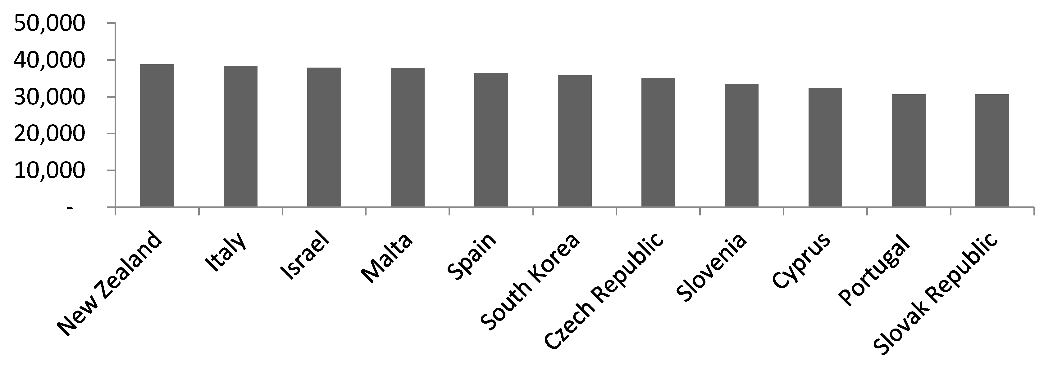
Figure 2.
Monthly returns of the value and growth indexes. Source: Bloomberg.
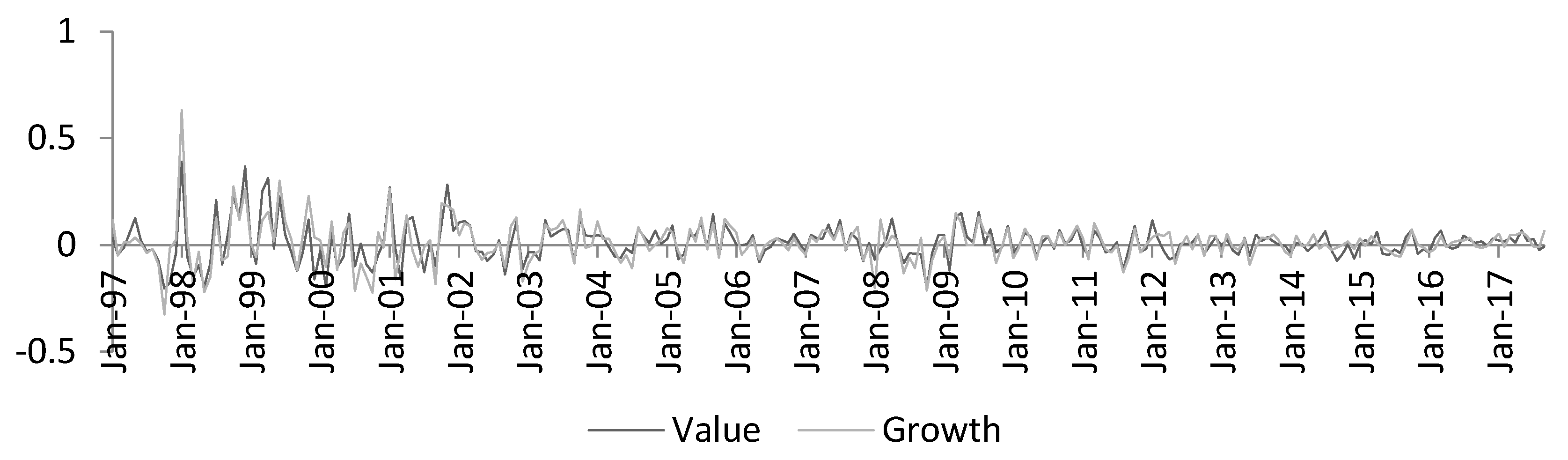
Figure 3.
Monthly returns of the small, mid and large cap indexes. Source: Bloomberg.

Figure 4.
Portfolio value; PE equal weight.

Figure 5.
Portfolio value; PE market capitalization weight.

Figure 6.
Portfolio value; PB equal weight.
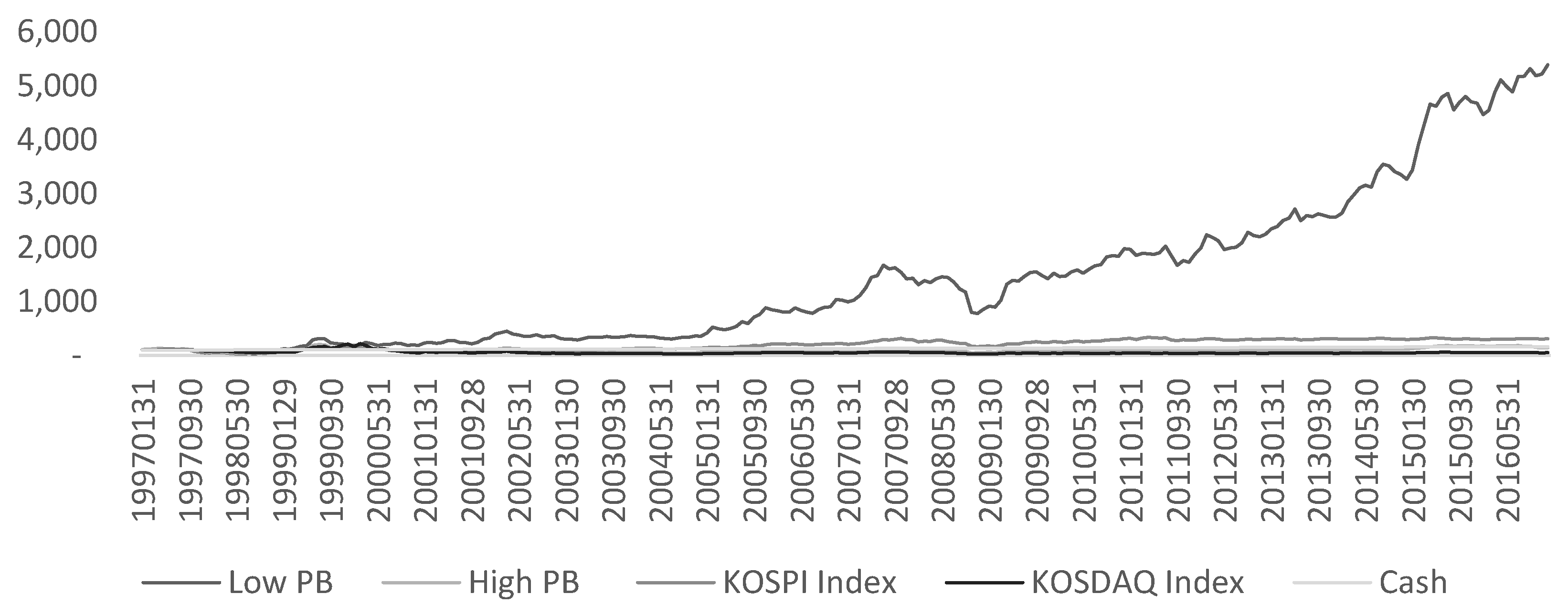
Figure 7.
Portfolio value; PB market capitalization weight.
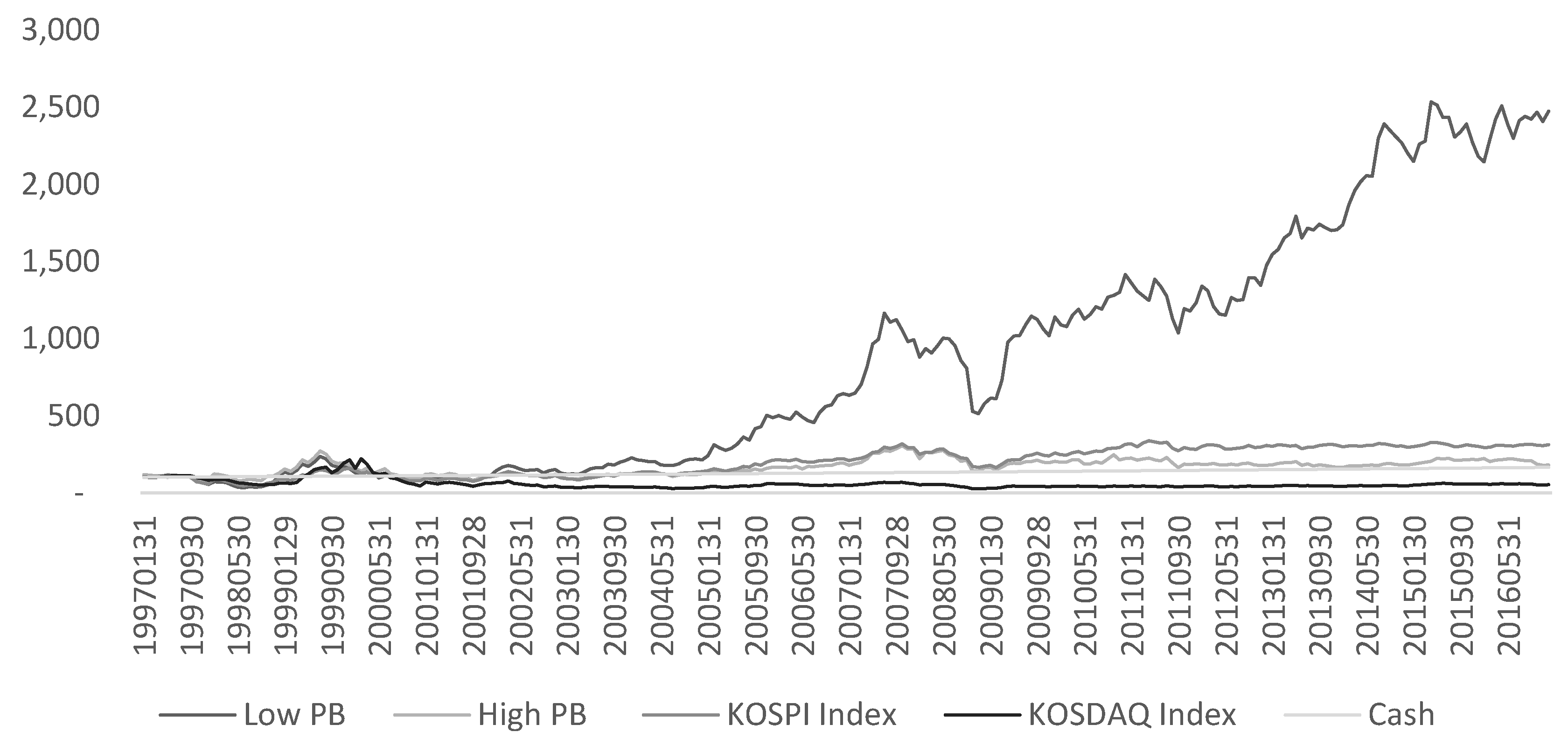
Figure 8.
Portfolio value; 5-year average sales growth–equal weight.

Figure 9.
Portfolio value; 5-year average sales growth–market capitalization weight.

Figure 10.
Portfolio value; Cash flow per share–equal weight.

Figure 11.
Portfolio value; Cash flow per share–Market capitalization weight.

Figure 12.
12-month trailing correlation of low and high PE portfolios.

Figure 13.
12-month trailing correlation of low and high P/B portfolios.

Figure 14.
12-month trailing correlation of low and high cash flow per share portfolios.

Figure 15.
12-month trailing correlation of low and high 5-year average growth sales portfolios.
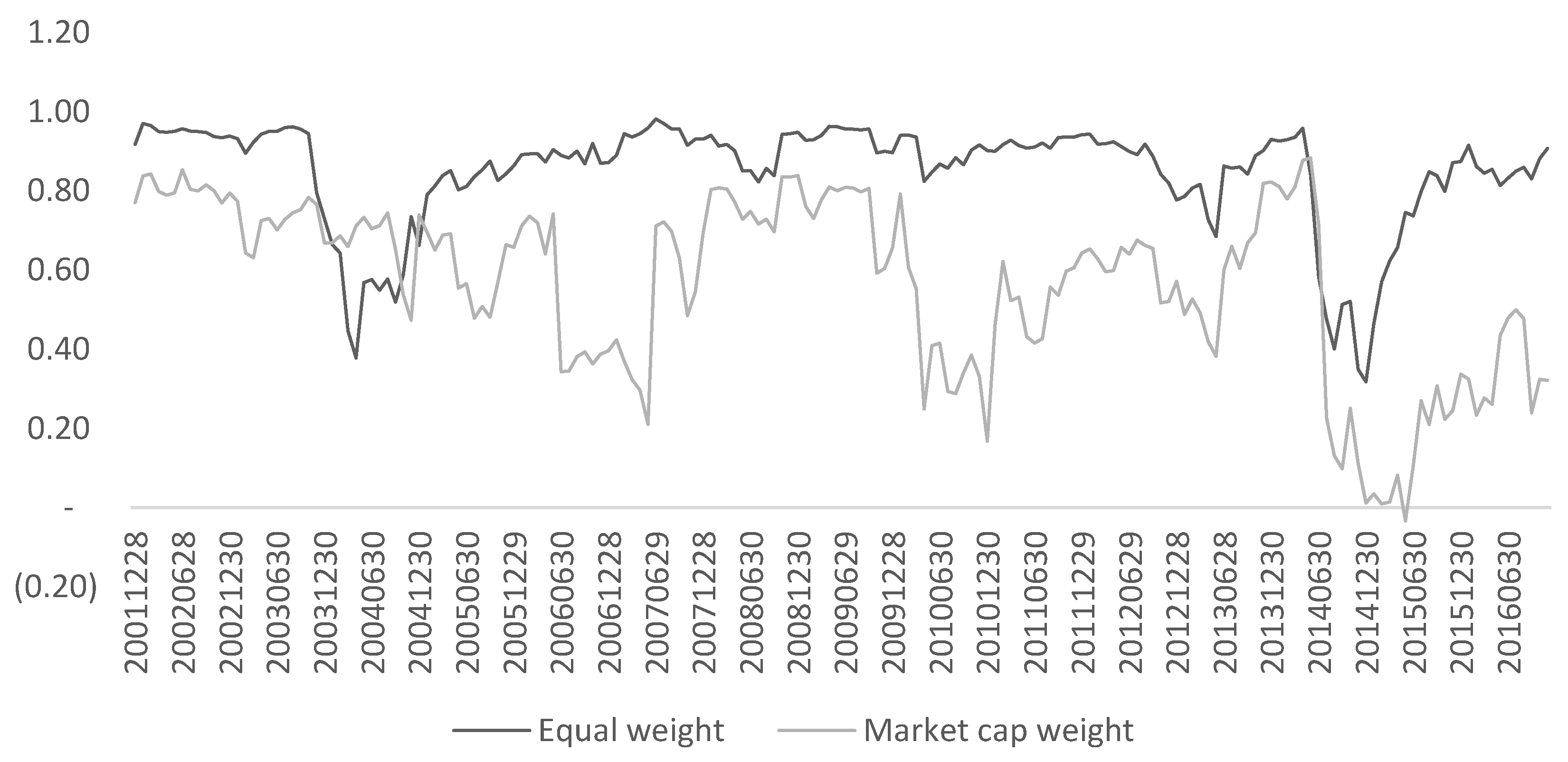
Table 1.
Anderson Darling test for the value and growth indexes (1997–2016).
| Index | p | H |
|---|---|---|
| Value | 0.0005 | 1 |
| Growth | 0.0005 | 1 |
Table 2.
Anderson Darling tests for the large, mid and small cap indexes (2010–2016).
| Index | p | H |
|---|---|---|
| Large | 0.7031 | 0 |
| Mid | 0.9600 | 0 |
| Small | 0.9350 | 0 |
Table 3.
Wilcoxon test comparing the returns of the size indexes (2010–2016).
| Indexes | p | H |
|---|---|---|
| Large–Mid | 0.6467 | 0 |
| Large–Small | 0.9709 | 0 |
| Mid–Small | 0.6882 | 0 |
Table 4.
Wilcoxon test comparing the returns of the size indexes (Yearly).
| Year | Large–Mid | Large–Small | Mid–Small | |||
|---|---|---|---|---|---|---|
| p | H | p | H | p | H | |
| 2010 | 0.795 | 0 | 0.583 | 0 | 0.544 | 0 |
| 2011 | 1.000 | 0 | 0.665 | 0 | 0.840 | 0 |
| 2012 | 0.583 | 0 | 0.403 | 0 | 0.795 | 0 |
| 2013 | 0.840 | 0 | 0.885 | 0 | 0.977 | 0 |
| 2014 | 0.977 | 0 | 0.403 | 0 | 0.371 | 0 |
| 2015 | 0.624 | 0 | 0.175 | 0 | 0.544 | 0 |
| 2016 | 0.089 | 0 | 0.100 | 0 | 0.931 | 0 |
Table 5.
Kruskal Wallis test comparing the returns of the size indexes (2010–2016).
| Indexes | p | H |
|---|---|---|
| Large–Mid | 0.6455 | 0 |
| Large–Small | 0.9696 | 0 |
| Mid–Small | 0.6870 | 0 |
Table 6.
Kruskal Wallis test comparing the returns of the size indexes (Yearly).
| Year | Large–Mid | Large–Small | Mid–Small | |||
|---|---|---|---|---|---|---|
| p | H | p | H | p | H | |
| 2010 | 0.7728 | 0 | 0.5637 | 0 | 0.5254 | 0 |
| 2011 | 0.9999 | 0 | 0.6442 | 0 | 0.8174 | 0 |
| 2012 | 0.5637 | 0 | 0.3865 | 0 | 0.7728 | 0 |
| 2013 | 0.8174 | 0 | 0.8625 | 0 | 0.9540 | 0 |
| 2014 | 0.9540 | 0 | 0.3865 | 0 | 0.3556 | 0 |
| 2015 | 0.6033 | 0 | 0.1659 | 0 | 0.5254 | 0 |
| 2016 | 0.0833 | 0 | 0.0941 | 0 | 0.9081 | 0 |
Table 7.
Wilcoxon signed rank test comparing the returns of the size indexes (2010–2016).
| Indexes | p | H |
|---|---|---|
| Large–Mid | 0.5412 | 0 |
| Large–Small | 0.9644 | 0 |
| Mid–Small | 0.6332 | 0 |
Table 8.
Wilcoxon signed rank test comparing the returns of the size indexes (Yearly).
| Year | Large–Mid | Large–Small | Mid–Small | |||
|---|---|---|---|---|---|---|
| p | H | p | H | p | H | |
| 2010 | 0.7334 | 0 | 0.6772 | 0 | 0.1763 | 0 |
| 2011 | 0.7910 | 0 | 0.6772 | 0 | 0.1099 | 0 |
| 2012 | 0.4697 | 0 | 0.3013 | 0 | 0.4697 | 0 |
| 2013 | 0.8501 | 0 | 0.9097 | 0 | 0.6772 | 0 |
| 2014 | 0.8501 | 0 | 0.3804 | 0 | 0.0923 | 0 |
| 2015 | 0.3804 | 0 | 0.1763 | 0 | 0.3013 | 0 |
| 2016 | 0.0640 | 0 | 0.0771 | 0 | 0.7910 | 0 |
Table 9.
Wilcoxon test comparing the returns of the style indexes (all data).
| Indexes | p | H |
|---|---|---|
| Value–Growth | 0.6533 | 0 |
Table 10.
Wilcoxon test comparing the returns of the value and growth indexes (yearly).
| Year | p | H | Year | p | H |
|---|---|---|---|---|---|
| 1997 | 0.7950 | 0 | 2007 | 1.0000 | 0 |
| 1998 | 0.9770 | 0 | 2008 | 0.7075 | 0 |
| 1999 | 0.4357 | 0 | 2009 | 0.7950 | 0 |
| 2000 | 0.9770 | 0 | 2010 | 0.9770 | 0 |
| 2001 | 0.8399 | 0 | 2011 | 0.8852 | 0 |
| 2002 | 1.0000 | 0 | 2012 | 0.2602 | 0 |
| 2003 | 0.9310 | 0 | 2013 | 0.9770 | 0 |
| 2004 | 0.7075 | 0 | 2014 | 0.4705 | 0 |
| 2005 | 0.8852 | 0 | 2015 | 0.9310 | 0 |
| 2006 | 0.7075 | 0 | 2016 | 0.5067 | 0 |
Table 11.
Kruskal Wallis test comparing the returns of the style indexes (all data).
| Indexes | p | H |
|---|---|---|
| Value–Growth | 0.6531 | 0 |
Table 12.
Kruskal Wallis test comparing the returns of the value and growth indexes (yearly).
| Year | p | H | Year | p | H |
|---|---|---|---|---|---|
| 1997 | 0.7728 | 0 | 2007 | 1.0000 | 0 |
| 1998 | 0.9540 | 0 | 2008 | 0.6861 | 0 |
| 1999 | 0.4189 | 0 | 2009 | 0.7728 | 0 |
| 2000 | 0.9540 | 0 | 2010 | 0.9540 | 0 |
| 2001 | 0.8174 | 0 | 2011 | 0.8625 | 0 |
| 2002 | 1.0000 | 0 | 2012 | 0.2482 | 0 |
| 2003 | 0.9081 | 0 | 2013 | 0.9540 | 0 |
| 2004 | 0.6861 | 0 | 2014 | 0.4529 | 0 |
| 2005 | 0.8625 | 0 | 2015 | 0.9081 | 0 |
| 2006 | 0.6861 | 0 | 2016 | 0.4884 | 0 |
Table 13.
Wilcoxon signed rank test comparing the returns of the style indexes (all data).
| Indexes | p | H |
|---|---|---|
| Value–Growth | 0.7353 | 0 |
Table 14.
Wilcoxon signed rank test comparing the returns of the value and growth indexes (yearly).
| Year | p | H | Year | p | H |
|---|---|---|---|---|---|
| 1997 | 0.8501 | 0 | 2007 | 0.3394 | 0 |
| 1998 | 0.7334 | 0 | 2008 | 0.2334 | 0 |
| 1999 | 0.1763 | 0 | 2009 | 0.4697 | 0 |
| 2000 | 1.0000 | 0 | 2010 | 0.9697 | 0 |
| 2001 | 0.7334 | 0 | 2011 | 0.9697 | 0 |
| 2002 | 0.9097 | 0 | 2012 | 0.5693 | 0 |
| 2003 | 0.7910 | 0 | 2013 | 0.7334 | 0 |
| 2004 | 0.5693 | 0 | 2014 | 0.2661 | 0 |
| 2005 | 0.9097 | 0 | 2015 | 0.9097 | 0 |
| 2006 | 0.6221 | 0 | 2016 | 0.3013 | 0 |
© 2018 by the author. Licensee MDPI, Basel, Switzerland. This article is an open access article distributed under the terms and conditions of the Creative Commons Attribution (CC BY) license (http://creativecommons.org/licenses/by/4.0/).
Share and Cite
MDPI and ACS Style
Perez, G.“.A. Value Investing and Size Effect in the South Korean Stock Market. Int. J. Financial Stud. 2018, 6, 31. https://doi.org/10.3390/ijfs6010031
AMA Style
Perez G“A. Value Investing and Size Effect in the South Korean Stock Market. International Journal of Financial Studies. 2018; 6(1):31. https://doi.org/10.3390/ijfs6010031
Chicago/Turabian StylePerez, Gerardo “Gerry” Alfonso. 2018. "Value Investing and Size Effect in the South Korean Stock Market" International Journal of Financial Studies 6, no. 1: 31. https://doi.org/10.3390/ijfs6010031
Note that from the first issue of 2016, this journal uses article numbers instead of page numbers. See further details here.