Asymptotic Expansion of Risk-Neutral Pricing Density

Department of Economics and Finance, University of Greifswald, 17489 Greifswald, Germany
Int. J. Financial Stud. 2018, 6(1), 30; https://doi.org/10.3390/ijfs6010030
Submission received: 14 December 2017
/
Revised: 7 February 2018
/
Accepted: 27 February 2018
/
Published: 12 March 2018
(This article belongs to the Special Issue Recent Developments in Numerical Methods for Option Pricing)
Abstract
:A new method for pricing contingent claims based on an asymptotic expansion of the dynamics of the pricing density is introduced. The expansion is conducted in a preferred coordinate frame, in which the pricing density looks stationary. The resulting asymptotic Kolmogorov-backward-equation is approximated by using a complete set of orthogonal Hermite-polynomials. The derived model is calibrated and tested on a collection of 1075 European-style ‘Deutscher Aktienindex’ (DAX) index options and is shown to generate very precise option prices and a more accurate implied volatility surface than conventional methods.
Keywords:
Kolmogorov-backward-equation; asymptotic expansion; Hermite-polynomials; implied volatility surfaceJEL Classification:
C61; G131. Introduction
Modern financial markets contain a rich variety of liquidly traded vanilla and exotic contracts, contingent on a large number of underlyings. A key requirement in such dense markets is the consistent valuation of novel and existing derivative contracts to rule out arbitrage opportunities. Because of market incompleteness, there is no unique risk-neutral Martingale measure, and hence no unique risk-neutral probability density for valuing such contracts. The necessary information on risk premia has to be extracted from the observed derivative prices. This is accomplished by calibrating a specific model to the available data. Usually, such models are stochastic path models for the underlying, which are calibrated to fit observed option prices (prominent examples are Bates 1996; Heston 1993; Kou 2002), or observed Black–Scholes implied volatilities (for example the SABR model of Hagan et al. 2002). A closely related and successful approach is to parameterize the implied volatility smile and skew, for example as suggested in (Gatheral 2004, 2006, p. 37), for different times to maturity, and to smoothly connect the time slices, eliminating calendar spread arbitrage opportunities. Sufficient conditions for elimination of static arbitrage are provided in Carr and Madan (2005), and an efficient method for computing arbitrage-free implied volatility surfaces was introduced by Fengler (2009).
A conceptionally different idea is to estimate the arbitrage-free pricing density directly from available European plain vanilla call prices. This approach is based on the observation of Breeden and Litzenberger (1978) that the pricing density is given by the undiscounted second derivative of the European plain vanilla call price. Some suggested methods of this kind can be found in the works of Ait-Sahalia and Duarte (2003); Ait-Sahalia and Lo (1998); Bondarenko (2003); Figlewski (2010); Hlavka and Svojik (2009); Huynh et al. (2002); Yatchew and Haerdle (2006). A recent approach by Filipović et al. (2012) stipulates a so-called ‘Master Equation’ for the time evolution of a fairly general class of admissible pricing densities, and provides some examples. Even though the idea is vaguely similar, the method suggested in this paper is entirely different.
The key idea in the approach suggested here is to generate modified dynamics of the arbitrage-free pricing density by asymptotic expansion around the classical Black-Scholes dynamics of complete markets. Asymptotic analysis has proven a very potent tool in deriving new results over the last fifteen years (see for example Basu and Ghosh 2009; Hagan et al. 2002; Kim 2002; Mazzoni 2015; Medvedev and Scaillet 2003; Uchida and Yoshida 2004; Whalley and Willmot 1997) whenever certain parts of a problem can be assumed as small. The first step in this approach is to express the complete market dynamics of the risk-neutral pricing density in a new coordinate frame, where it looks stationary. In such a frame, the transition density has to be Dirac’s delta function. If the dynamics of an incomplete market do not deviate too heavily from those of the complete market, it can be assumed that the singular transition density is only a first-order approximation of a narrow transition kernel of the order for short time intervals . Pursuing this avenue leads to an asymptotic version of the Kolmogorov-backward-equation for the excess dynamics of the incomplete market. This partial differential equation (PDE) can be solved approximately with the help of a complete set of orthogonal functions and a few additional assumptions, primarily related to the smallness of the asymptotic terms.
The idea of using a complete set of orthogonal functions to represent an unknown probability density function is not new. Ait-Sahalia (2002) advanced the Gram–Charlier-series of type A, utilizing Hermite-polynomials orthogonal to the weighting function to represent an unknown probability density. This approach has the advantage that the expansion has a leading Gaussian term and the coefficients are proportional to the cumulants of the approximated density. Since then, Hermite-polynomials or cumulant expansions, respectively, were also used in derivative pricing (c.f. Habtemicael and SenGupta 2016a, 2016b; Mazzoni 2010; Xiu 2014). Even though the suggested approach is superficially similar to the work of Xiu (2014), it is based on a completely different idea and has very different implications. Xiu (2014) follows the classical way of representing the unknown pricing density by a Gram-Charlier-series and solving the resulting Feynman-Kac PDE. There are two major drawbacks involved. Firstly, following the derivation of Ait-Sahalia (2002), there are powers of the infinitesimal generator of the original diffusion involved in the computation of the cumulants. Those terms are exceedingly complicated and have to be evaluated with a computer algebra system, but more importantly, they are model-dependent. Secondly, the Gram-Charlier-series is not an asymptotic series in the proper sense (for an excellent discussion of this issue see Blinnikov and Moessner 1998). Thus, the more expansion terms are involved, the faster the series degenerates, even if the deviation from normality is merely moderate. The approach suggested here is completely model-independent. It derives an asymptotic version of the Kolmogorov-backward-PDE from first principles. This equation contains unknown functions to be represented in terms of an orthogonal series expansion using Hermite-polynomials, orthogonal with respect to the weighting function . This version of the Hermite-polynomials is much more robust with respect to deviations from normality and is usually only limited by numerical issues. Of course the coefficients of the orthogonal series expansion have no connection to the cumulants of the unknown density function. They are instead determined explicitly from a system of ordinary differential equations and are related to the empirically observed deviations from normality.
Several aspects of the resulting valuation method are investigated, based on a collection of 1075 European-style index options, contingent on the ‘Deutscher Aktienindex’ (DAX) index. Because of the decreasing interest rate term structure and some other exceptional market conditions due to the Euro crisis, and the large number of available contracts with bid-offer spreads below , the DAX index is an optimal laboratory to survey the properties of the suggested method. In particular, it is shown that it generates very precise in- and out-of-sample option prices, and that the characteristics of the implied volatility surface are reconstructed quite satisfactorily over wide ranges of moneyness and time to maturity. The remainder of the paper is organized as follows:
Section 2 sets the scene for the asymptotic expansion of the incomplete market transition kernel. Departing from the classical risk-neutral geometrical Brownian motion and the corresponding time-dependent probability density function, the stationary coordinate frame transformation is introduced. Subsequently, the transition density is asymptotically expanded to derive the general equation for the excess dynamics due to market incompleteness. Finally, the unknown functions in this equation are expressed in a suitable way for model fitting.
In Section 3 a complete set of orthogonal functions based on Hermite-polynomials is introduced, in order to approximately solve for the incomplete market dynamics. In the process, the partial differential equation is transformed into a solvable linear system of ordinary differential equations. Furthermore, the constituents can be computed recursively. It turns out that there is an intimate connection between the resulting formula for the time-dependent pricing density and option pricing by quadrature methods, which is also elaborated at the end of this section.
In Section 4 the resulting model is calibrated to market data. To this end, a quadratic objective function is defined, which is to be minimized. It is shown that the gradient of this objective function can be computed analytically, which is instrumental for parameter estimation with quasi-Newton methods. The results of the calibration procedure are discussed and compared across different model configurations. The order of relative pricing error in the suggested framework is reduced to the order of bid-offer spreads of the contracts in the calibration sample.
Section 5 investigates the quality of the implied volatility surface, generated by the calibrated model. Because many contract types are highly vega-sensitive, implied volatility characteristics are of particular importance. The suggested method is benchmarked against two state-of-the-art approaches: the SABR model of Hagan et al. (2002) and the stochastic volatility inspired (SVI) parametrization of the local volatility surface by Gatheral and Wang (2012), associated with a most likely path approximation. It is shown that both alternatives provide an inferior fit, compared to the conditional density approach suggested here.
In Section 6 a collection of 171 European-style capped call and put options are valued. Those options were not included in the calibration sample and hence form an independent validation sample. It is also shown how to value contracts with arbitrary payoff functions with Monte Carlo simulation. This matter is not trivial, because one is not able to draw directly from the arbitrage-free pricing distribution. Two alternatives—a multinomial approximation and an importance sampling method—are detailed. The results are again in favor of the conditional pricing density approach.
Section 7 concludes the paper with a summary of the results and a discussion of the pros and cons of the suggested method.
2. Asymptotic Expansion of the Pricing Density
Assume a probability space is fixed, equipped with a natural filtration , generated by the P-measurable price processes of the underlying and all derivatives contingent on it, and with all null sets contained in . Classical theory (Black and Scholes 1973; Black 1976) entails a unique risk-neutral Ito-process
under the T-forward measure , such that the value of an arbitrary vanilla type contract1, contingent on its payoff at maturity, is given by
In Equation (2), is a zero-coupon bond with unit face value maturing at time T, and is the forward price of the underlying S. The classical model is rejected with overwhelming empirical proof, partly because of oversimplified assumptions, for example the volatility in (1) is assumed constant and known, and partly because it does not properly reflect all sources of (systematic) risk. An example for the latter are jump risks. An attempt to overcome this problem is the jump diffusion model of Merton (1976) but in order to preserve market completeness and hence the uniqueness of the pricing measure, jump risks have to be considered purely idiosyncratic, which is barely a realistic assumption (cf. Lewis 2002). Other risks not accounted for are liquidity risks, default risks, and even model risks.
Even though other models like those of Heston (1993), Bates (1996) or Hagan et al. (2002)—which are designed to work properly in incomplete markets after calibration to market data—are extraordinary successful, results of the Black–Scholes model are approximately correct in many situations. Therefore, it seems quite natural to expand around the Black–Scholes solution to obtain a valid result in an incomplete market setup, as long as the deviation from completeness is not too extreme. To set the scene for such an expansion, the time-dependent probability density of the path model (1) is subjected to some basic transformations.
Let be the logarithm of the forward price of the underlying. Due to Ito’s lemma, the (risk-neutral) probability density function of x is governed by the Fokker–Planck-equation
with indicating Dirac’s delta function. The solution to this PDE problem can be obtained with standard methods like Fourier-transform and is known to be
Note that this density is singular at , which is not a problem because one valid definition of the delta function is in terms of the limit of a sequence of functions like Equation (4), , (cf. Lighthill 1980, chp. 2.2). One merely has to remember that the initial density is not given by Equation (4), but by its limit. This is an important point for the following transformation, which is singular at , but the limit relation still holds. Define new coordinates and , with
After the transformation , the risk-neutral probability density is , with indicating the standard normal probability density function. In this new coordinates the probability density is stationary and standardized, making this particular coordinate system appear more fundamental than all others (a proof of the stationarity of the transformation is provided in Appendix A). It serves indeed as a laboratory frame for investigating the deviations from the Black–Scholes solution in that the asymptotic expansion is constructed in this frame. The PDE problem in the coordinates, corresponding to the problem in Equation (3) in the -coordinates, is
As discussed previously, one has to remember that is only the limit of when , because the coordinate transformation is singular at .
The universal statement implied by Equation (6) is that in the Black-Scholes world, the standardized risk neutral pricing density is Gaussian and remains Gaussian at all times. One would expect the pricing density to deviate from this stationary density in incomplete markets, reflecting the unhedgeable systematic risk structure of such markets. This deviation is implemented in the next paragraph by asymptotic expansion.
2.1. Asymptotic Deviation from Market Completeness
In order to determine the mechanism for the deviation from the Black–Scholes solution, write the pricing density in terms of the law of total probability
Observe that in the Black–Scholes framework the transition density has to be given by in order for Equation (7) to obey the degenerate dynamics in Equation (6). The key idea of the approach is to assume that in incomplete markets this transition density deviates from the delta function, and that the systematic risk structure, however it may be composed, is encoded in the way the transition kernel deviates.
To make this idea more precise, account for some boundary conditions. First, in the limit the transition density has to be the delta function because Equation (7) becomes an identity. Thus, one can conclude that the space–time interval, occupied by the transition kernel, has to be proportional to for short times (). Second, the Black–Scholes framework often generates useful approximative results, thus the spatial expanse of the transition kernel per unit of should be small, indicated by . Putting these arguments together, one concludes that the space–time volume occupied by the transition kernel should be roughly of order . Next, Taylor-expand the initial density around z to obtain
and define the auxiliary functions
Now Equation (7) can be expressed in terms of a Taylor-like series expansion
which is very similar to the Kramers–Moyal-backward-expansion (Risken 1989, chp. 4.2). However, this similarity is only superficial, because the integration in Equation (9) is with respect to the conditioning variable y, which means that is not a transition moment and Equation (10) is merely a formal series expansion. Because the transition kernel becomes the delta function in the limit , it follows immediately that and for all . If is sufficiently smooth, which is a very mild requirement, can be expanded itself around and one obtains
for , with the yet unknown functions . Remember that the transition kernel occupies a space–time volume of order . Therefore, the n-th order auxiliary function has to be roughly of order . Putting all pieces together one obtains
Clearly one cannot compute the entire sum on the right hand side of Equation (12) and thus usually a decision has to be made with respect to the terms to abandon. Often terms up to are considered and all higher orders are neglected. The situation here is different. Because is a probability density, which by definition is nonnegative everywhere, the Pawula theorem applies (cf. Risken 1989, chp. 4.3). This remarkable theorem proves that considering the first two terms of the expansion in Equation (12) is the best possible approximation available, without considering the last term at infinity. In this case, the contribution from higher-order terms diminishes, because of their order in . Hence, if it is assumed that the contribution of terms of infinite powers of vanishes, it can be concluded that the approximation including terms has to be exact. One therefore obtains instead of Equation (6) an asymptotic version of the Kolmogorov-backward-equation
with the yet unknown functions and , encoding all information about the deviation of the systematic risk structure from the classical Black–Scholes world. The next step is to determine these unknown functions.
2.2. Decoding Market Information
Because of the extremely rich structure of systematic market risk, model-guided determination of the functions , apart from a few special cases discussed subsequently, may be generally impossible. Thus, some assumptions have to be made, allowing for the tractable incorporation of observed empirical information. The following discussion is focused on the function but all arguments carry over to the term. The first assumption is that the function is time separable and that it has the form
where the small number is soaked up in the function . There are several reasons for this particular choice:
- Recall that the coordinates are already dynamically scaled and hence, only the excess dynamics are to be modeled. These dynamics are governed by additional risk structure, unfolding over time. For example, liquidity risk is of minor importance in short-term scenarios but has to be accounted for over longer holding periods. Jump risk contributes to the steepness of the short term implied volatility smile, but does not affect the long-term structure. If all the additional risk structure is fully deployed, the deformation of the pricing density is completed. This behavior is induced in Equation (14).
- This particular choice reproduces some known standard results. For example, in the limit one obtains the classical Black-Scholes solution. As a second example, imagine a completely illiquid market, such that even static hedging is not possible. The choice and yields the solution , which after retransformation to -coordinates is immediately recognized as the time-honored actuarial pricing density under P (cf. Derman and Taleb 2005).
- The plain exponential model for the time dependence is the most parsimonious parametrization of the problem. By this choice, the subsequent calibration procedure is simplified considerably. Even if this model is oversimplified in that it implies the whole risk structure to unfold in a synchronized way, it seems to be at least a good starting point.
The second assumption, essential for recursive computation of the pricing density as shown in the next section, is that is sufficiently smooth to be expanded into a power series, . This is again a relatively mild technical condition. The whole problem now becomes
again with initial condition . Obviously, the sums in Equation (15) cannot be calculated either. However, one can expect very few coefficients to contribute to the sums for the following line of reasoning: Departing from the initial standard Gaussian density, roughly of the probability mass is located at . The outer region of the density would be exposed to violent deformations if for large k the term or contributes, respectively. Because the Black–Scholes solution is a good approximation, the deviation from normality has to be moderate, and hence higher order coefficients have to be minute.
3. Computation of the Pricing Density
In order to solve the PDE (15) at least approximately, the pricing density is rewritten in terms of a complete orthogonal system
In Equation (16), represents the n-th Hermite-polynomial, orthogonal to the weight function defined by . Observe that this is neither Gram–Charlier-, nor Edgeworth-expansion2, which are both constructed from orthogonal functions with respect to the weight function , but a generalized Fourier-series with correctly normalized orthogonal functions, such that
holds, with the Kronecker-delta . Observe further that every orthogonal function , apart from a constant, contains a standard Gaussian term. Thus, this orthogonal system is particularly well-suited for the problem at hand. Of course, one has to fix a maximum number of expansion terms to be included, but for small deviations from the normal distribution the series converges well (Blinnikov and Moessner 1998).
The advantage offered by the Fourier-series expansion is the separation of time and spatial dependence. Using this advantage, the time dependent values of the Fourier-coefficients in Equation (16) can be computed by solving an ordinary first-order differential equation system.
Proposition 1.
The Fourier-coefficients for n = 0, 1, 2, …are determined by the solution of the infinite dimensional matrix/vector differential equation
where is the vector containing the coefficients , , , and so forth.
Proof.
Computing the nth Fourier-coefficient and using Equation (15), one obtains
Again substituting the complete orthogonal system in Equation (16) for the density function yields
Identifying the integrals as elements
of the matrices and , the problem in Equation (20) can be rewritten in matrix/vector form as
which is the desired result. ☐
It turns out that the matrices and can be computed recursively, exploiting particular properties of the Hermite-polynomials contained in the orthogonal functions. This is a very convenient fact, because recursive patterns can be efficiently implemented on a computer. The procedures are detailed in the next paragraph.
3.1. Recursive Computation of the Matrix Entries
The computation scheme for the entries of the matrices and is given in the subsequent proposition.
Proposition 2.
For or , the following recursion holds
with initial conditions
Proof.
In order to compute the entries of the matrices and , two essential properties of Hermite-polynomials are used. First, the recursive relation between the polynomials and their derivatives , and second, the recurrence relation (cf. Abramowitz and Stegun 1970, p. 782). From property number 1 and the definition of the orthogonal functions (16), one immediately obtains
and thus for ,
follow from the orthonormality in Equation (17). From the recurrence relation, one obtains in terms of the orthogonal functions
which yields the recursive relation
for both matrices and , respectively. ☐
Note that in the exact case of Equation (18) there are infinitely many matrices of infinite dimensions. Thus, one has to decide how many terms of the orthogonal expansion to include in the computation, and which terms of the power series expansion of the unknown functions and to abandon. The former is primarily a technical question of convergence of the Fourier-series, while the latter is a question of approximating the dynamics of the risk structure correctly. Both are strongly related to the degree of deviation from normality, but only the coefficients and immediately affect the model calibration process. Because it is impossible to determine beforehand which terms of both expansions might be neglected, different alternatives are compared in Section 4.
3.2. Fourier-Coefficients and Pricing Density
Once the approximations are fixed, the Fourier-coefficients can be calculated immediately. Knowing all constituents of the matrices and from the recursive scheme in Proposition 2, the system of ordinary differential Equation (18) can be solved
with and for , and denoting the matrix exponential. There are several alternative methods for calculating a matrix exponential (cf. Moler and van Loan 2003), such that Equation (29) is quite explicit. Thus, the whole pricing density can be approximated by
or after retransformation into -coordinates
The retransformation however is of little practical use, because the payoff function of an arbitrary contingent claim can be easily transformed into -coordinates.
Determination of the power series coefficients and is a matter of calibration to market data and has to be done numerically. Completing this procedure results in a model for the time evolution of the arbitrage-free pricing density, conditional on the information set , representing the market view of future risks as it stands today. There is no requirement for interpolation or even extrapolation like in case of nonparametric estimates of implied volatility surfaces. However, one big assumption has been made about the time separability of the unknown functions in Equation (13) and the temporal structure of risks in Equation (14). As stated above, this assumption may be oversimplified, leaving a margin for enhancement of the model fit, at the cost of increased complexity.
3.3. Pricing Vanilla Contracts
One major drawback of the pricing density (Equations (30) and (31)) is that analytical valuation of vanilla contracts is much harder than in the Black–Scholes case, where all higher polynomial terms vanish. However, there is a very convenient and computationally efficient way of pricing derivatives numerically, based on Gauss–Hermite-quadrature. The value of a vanilla contract at time , maturing at time is given by
The connection between the forward price and the stock price at is given by . Because has a leading standard normal density function, the integral can be approximated by a weighted sum
with indicating the Gauss–Hermite-quadrature weights and the corresponding quadrature points. All necessary information about weights and points can be extracted from the eigensystem of the matrix,
cf. Golub (1973). The eigenvalues of M are the quadrature points, whereas the corresponding weights are given by the squared first components of the corresponding normalized eigenvectors. The quadrature is exact for polynomials up to a degree of , indicating an intimate relation between the Hermite-polynomials involved and the necessary number of quadrature points. However, the payoff function of plain vanilla calls and puts is not polynomial, leaving Equation (33) as an approximation.
Observe that not all terms in (33) rely on the full information of an individual contract. The Fourier-coefficients for example only depend on the time to maturity of the contract, whereas the Hermite-polynomials do not depend on the contract at all. This suggests an efficient way of pricing individual contracts. Defining the vector with components and the matrix H, with , the fair value of the m-th contract is given by
where H has to be computed only once, and only once for each expiry of the whole set of contracts.
Equipped with both a model for the time evolution of the arbitrage-free pricing density and a method for pricing plain vanilla options in this framework, the next step is calibrating the model to market data.
4. Calibration to Market Data
The model calibration process primarily contains three more or less interdependent tasks:
- Determination of a sufficient number of Fourier-terms to be included in the approximation.
- Determination of the optimal model order and .
- Estimation of the model parameters based on the available empirical data.
The determination of the optimal number of Fourier-coefficients is only weakly related to the model order. It is primarily affected by the degree of deviation from normal. The more extensive the deviation is, the more terms are required for the orthogonal series expansion to converge. Theoretically, an arbitrary probability density can be approximated with sufficient precision by simply including enough expansion terms. Practically, numerical problems have to be considered if the desired density function deviates extensively from the standard normal. Because of finite numerical precision, at some point including additional terms is no longer beneficial because of rounding errors, effectively limiting the manageable degree of deviation from normal. Beyond this limit, artifacts like local negative densities may occur, which cannot be removed or may even be amplified by involving more expansion terms.
Both remaining determinations are strongly interdependent in that a sufficient model order can only be identified by judging the fit accomplished by different models. To this end, all potentially qualifying candidates have to be estimated. This is done numerically by a Newton–Raphson type scheme, associated with a prespecified objective function. Usually, a weighted sum of squared errors is to be minimized. In this case
is used, with indicating the observed mid-price of the m-th contingent claim. The weight factor may be chosen to reflect uncertainty induced by the magnitude of the bid-offer spread. In the study at hand, a large number of vanilla derivatives with spreads below was available, and thus the individual weight factors were set to for .
4.1. Data Description
In this analysis, a total of 433 European plain vanilla call options and 471 put options on the ‘Deutscher Aktien’ (DAX) index, quoted as per closing prices on 23 of July 2012, were available. In this case, 501 of these 904 contracts exhibited a bid-offer spread smaller or equal to and thus were used for model calibration. Additionally, 95 capped calls and 76 capped puts of the same date were used as a validation sample, although they could have been as well used for calibration3.
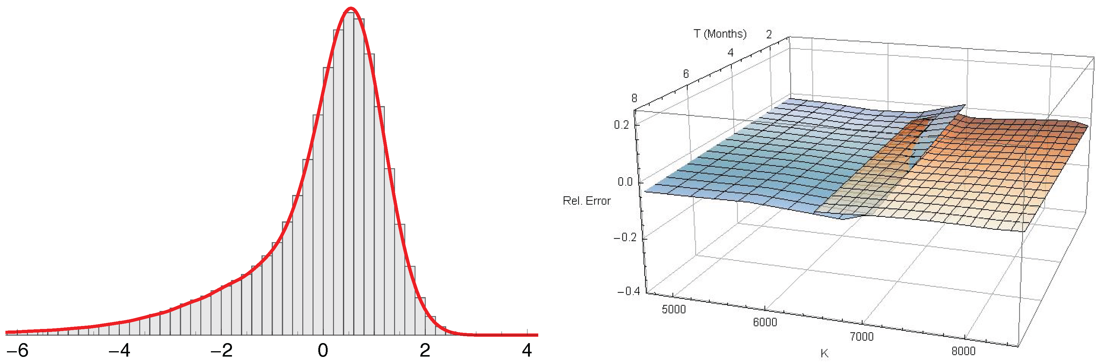
Figure 1 shows the relative pricing error under the Black–Scholes model for the 501 low spread contracts. The DAX index itself was quoted at points and the annualized at-the-money (ATM) implied volatility was about .
The interpolated call (blue) and put (red) surfaces in Figure 1 indicate that the relative error under Black–Scholes is moderate for in-the-money contracts, but grows formidable for out-of-the-money contracts. By using the right pricing density, both surfaces should be flattened out in time-to-maturity, as well as in moneyness direction.
The term structure and hence the prices of zero-coupon bonds of different maturities were extracted from the calibration sample as well by using put-call parity. After simple algebraic manipulations the bond price is explicitly given by
The yield curve extracted from the zero-coupon bond prices is inverted, falling from a return for 4 weeks time to maturity to approximately for an 18-month bond. This shape of the yield curve is due to the sovereign dept crisis, affecting the Euro area since 2010.
Based on the empirical data, the next step is calibrating the model and identifying a suitable model order. To this end, the whole set of parameters has to be estimated for different model alternatives.
4.2. Gradient of the Objective Function
Define the whole parameter vector , for a given model. A suitable estimate for can be obtained recursively, departing from a given initial configuration, by an iterative Newton–Raphson type scheme
In Equation (38) indicates an individual step size factor, determined by step halfing or trust region methods4, is a model Hessian, for example the identity matrix, resulting in a steepest descent algorithm, and is the gradient of the objective function, defined componentwise by . In the present analysis, the BFGS-method of Broyden (1970); Fletcher (1970); Goldfarb (1970); Shanno (1970) has been used, because it converges rapidly and no second derivatives are involved in the computation of the Hessian model. Thus, an analytical expression for the gradient of the objective function eliminates the need for finite difference approximations entirely. It turns out that such an expression can be derived, at least approximately. First, note that the partial derivative of the m-th term of the objective function in Equation(36), with respect to the j-th parameter is given by
where the approximate value of the contract (Equation (35)) was plugged in on the right-hand side of Equation (39). Obviously, the partial derivatives of Q are linear functions of the partial derivatives of the Fourier-coefficients given by Equation (29). They are given here as a proposition, the proof of which can be found in Appendix B.
Proposition 3.
The partial derivatives of the Fourier coefficient vector with respect to γ, and are given by
with indicating a block matrix and I the identity matrix.
Now, one is able to estimate different models and to compare their fit with respect to their model order and the residual square error.
4.3. Results of Model Calibration
Table 1 shows the results of the calibration process involving Fourier-coefficients, which turned out to be sufficient over all model orders. Each cell shows the residual root-mean-square error (RMSE) and the estimated standardized pricing density for contracts with time to maturity year. This is quite close to the stationary density for the most models. Obviously, the pricing density exhibits significant skewness and a pronounced left tail. The deviation from normal is excessive, resulting in invalid density estimates for some model candidates, indicated in gray in Table 1. The degeneration of the density estimates is due to the numerical limits of the orthogonal series expansion and could not be remedied in the present analysis by involving more Fourier-terms. Nevertheless, there are some valid and parsimonious candidates with small RMSE, like the -model.
Note that only models with even orders of are reported. This is due to the definition of the auxiliary functions in Equation (9). Because has a quadratic kernel, the function in Equation (11) should always be positive and thus a power series approximation of this function should be given by a polynomial of an even degree.
Figure 2 shows the relative pricing error for the calibration sample of 501 European plain vanilla call- and put-options. Obviously, the observed prices are reconstructed very precisely by the -model across the whole spectrum of moneyness and time to maturity. The exact parameter estimates for this model are , and . The root-mean-square error is , which is roughly the order of the bid-offer spreads of the valued contracts, suggesting that a sufficient fit has been accomplished. Therefore, the -model will be used in all subsequent benchmarks and numerical computations. All models were estimated with initial parameter setting and .
5. Implied Volatility Surface
In this section, the implied volatility surface, induced by the preferred model of Section 4, is analyzed and compared with other methods. The benefit of this investigation is twofold: on the one hand, volatility surfaces are a widely used tool for calibration of option pricing models to market data (for an excellent survey on this subject see Gatheral 2006). Their strengths and weaknesses are well known, and hence they are a convenient instrument for assessing the quality of the suggested method.
On the other hand, conditional pricing density estimation has one important conceptual drawback: since the whole density is globally conditioned on the information set , there is no way to get access to the transition density between times s and t for . This implies that valuation of path-dependent contracts by Monte Carlo simulation is not possible directly. However, this can be remedied by a kind of reverse engineering. One can use the Dupire-equation (Dupire 1994) to express the local volatility in terms of implied volatility (for details see for example Van der Kamp 2009, sct. 2.3). Simulation can then be performed using a geometrical Brownian motion under local volatility as model for the underlying.
The implied volatility surface is compared with the resulting surfaces of two standard approaches: the SABR model of Hagan et al. (2002) and a local volatility surfaces parametrization suggested by Gatheral and Wang (2012).
5.1. The SABR Model
Hagan et al. (2002) suggested a parametrization of implied volatility based on an asymptotic analysis of a parsimonious stochastic volatility model with singular perturbation methods. Their model is widely used because it is extraordinary easy to fit and generates correct implied volatility dynamics. Their general asymptotic formula is
with
Define the (inverse) log-moneyness and observe that the backbone of the implied volatility surface in Figure 3 (top left) does not drift vertically in time. Thus, one can set (for details see Hagan et al. (2002)). With these new parameters one obtains
with and as in Equation (43). This can be easily fitted to the calibration sample, and the resulting implied volatility surface is shown in Figure 3 (bottom right). It is however not entirely fair to calibrate the SABR model to the entire volatility surface, because it does not provide temporal dynamics by construction.
5.2. The SVI Parametrization of the Local Volatility Surface
In their paper, Gatheral and Wang (2012) suggest a parametrization of the local volatility surface, motivated by the structure of stochastic volatility models (‘stochastic volatility inspired’, SVI)
which is effectively a hyperbola in the log-strike k. There is an intimate connection between local and implied volatility. Implied variance is approximately the average over local variance
along the most likely path from to (cf. Gatheral 2006, chp. 3). Usually it is very difficult to compute this path and several approaches have been suggested (an incomplete list covers the work of Berestycki et al. 2002; Gatheral and Wang 2012; Gatheral et al. 2012; Guyon and Henry-Labordere 2011; Reghai 2006). However, it turns out that the straight line in the log-strike space is a reasonable first guess. Under this assumption, the line integral in Equation (46) can be expressed as
The integral in Equation (47) with respect to the SVI parametrization (45) can be computed analytically. Neglecting the constant of integration, one obtains
with
Differentiating (48) with respect to shows that the integral is indeed correct.
One can now fit the implied volatility surface to the calibration sample. The result is shown in Figure 3 (bottom left).
5.3. Results of the Benchmark
In order to compute the implied volatility surface, Black–Scholes implied volatilities were calculated for all out-of-the-money plain vanilla calls and puts, because they contain the most information about the volatility structure. This leaves 210 observations of the original low spread sample of 501 options, used for model calibration. This sample is also used for estimation of the SVI and SABR parameters in order to fit all models with identical information. The full sample of 904 contracts provides 613 observations of implied volatility. The particular model fits are also benchmarked regarding the full sample.
Figure 3 shows all estimated implied volatility surfaces. In particular, a first-order spline interpolation of the observation data is given in the upper left quadrant of Figure 3. The upper right surface is generated by the calibrated -model for the pricing density of Section 4. The lower left and lower right surfaces are generated by the SVI parametrization of the local volatility surface and by the SABR model, respectively. The meshing on the surfaces indicates slices of identical time to maturity (gray) and identical implied volatility (black), to emphasize the different features of the particular surfaces.
Obviously, none of the suggested models seems to manage the extremely sharp smile in the ultra short-term region, but this conclusion should be drawn with caution. Short-term out-of-the-money options are usually traded rarely and hence, quoted prices are not unconditionally reliable. In the data sample used in this analysis, information about the trading frequency was not provided. The surface based on the conditional pricing density (top right) nevertheless seems to cover the features of the empirical surface quit well, at least for . On the right edge it slightly underestimates the smile. The SVI parametrization (bottom left) generates an adequate long-term skew but an excessive smile for . It also misses the flattening of the surface for and . The SABR model surface in the bottom right quadrant seems to cover this particular feature but completely misses the short term structure of the volatility smile.
The difference between the observed implied volatility surface and the values generated by the three competitive approaches is shown in Figure 4, focusing on the central moneyness region. The surface meshing again indicates slices of identical time to maturity (gray) and identical implied volatility (black). The conditional density -model (top left of Figure 4) fits the observed implied volatility extremely accurately, whereas the SVI parametrization (top right) underestimates the mid- and long-term skew, and the SABR model (bottom center) does not generate the correct smile. It is evident from Figure 4 that the conditional density model generates the best implied volatility fit of all candidates.
Table 2 summarizes all models and compares the root-mean-square errors in both the calibration sample (CS) and the full sample (FS).
Again, the conditional pricing density model clearly provides the best fit, in particular in the calibration sample, where its root mean square error is smaller than half the RMSE of the SABR model.
6. Valuation under the Conditional Pricing Density Model
In this section an additional validation sample of 95 European vanilla capped calls and 76 puts of the same style is priced and analyzed. This is again accomplished numerically by Gauss–Hermite-quadrature methods like in Section 3.3. An alternative method for valuation is Monte Carlo simulation. Two different simulation approaches are introduced, one immediately related to quadrature methods, and the other based on importance sampling.
6.1. Capped Options Valuation
A European vanilla capped option is a unification of a long and a short position in the same plain vanilla type option, with identical time to maturity but different exercise prices, known as vertical spread. For example, the payoff of a European vanilla capped call option, with strike K and cap is
With this payoff function, the valuation Equations (33) and (35) respectively and immediately apply.
Figure 5 shows the relative misspricing under the classical Black-Scholes model (left) and the estimated -model of Section 4 (right).
Obviously, the pricing error is reduced dramatically. The root-mean-square error under the original Black–Scholes model is , whereas the remaining RMSE after conditional pricing density model fitting is . The spread of the analyzed capped options varies between and . Thus, the prices predicted by the -model match the observed mid-prices very closely, apart from a few short-term out-of-the-money contracts.
Nevertheless, the capped option valuation reveals a potential problem of the quadrature based numerical valuation procedure. The payoff function in Equation (50) clips a narrow interval out of the entire pricing density, which possibly contains only a small number of quadrature points. Therefore, numerical results may be inaccurate. There are two possible ways to improve the situation. First, one could simply increase the number of quadrature points involved in the numerical integration procedure. This idea breeds two new problems: On the one hand, only a fraction of the additional points is located in the relevant interval of the payoff function. On the other hand, there are a large number of quadrature points, with associated weights very close to zero, which means that the effect of a considerable amount of computed quadrature points on the valuation result is negligible. The latter problem at least can be resolved by pruning (cf. Jaeckel 2005).
Another alternative is Monte Carlo simulation. This is not a trivial task, because one is not able to draw from the arbitrage-free pricing distribution directly. Nevertheless, two indirect sampling methods are detailed in the next paragraph.
6.2. Monte Carlo Valuation Methods
A key requirement for Monte Carlo simulation is the ability to draw random numbers from the relevant probability distribution. Remember that the conditional pricing distribution for any time to maturity is given by its density function (Equation (30)) in -coordinates. This can be written as
with and again indicating Gauss–Hermite-quadrature weights and points, respectively. However, the second line of (51) is just an abusive way of writing a multinomial distribution function with values , occurring with probability
for . It is easy to draw from this multinomial distribution.
Figure 6 (left) shows the pricing density, generated with the -model (red), and the distribution of one million draws from the multinomial approximation as histogram (gray). A total of quadrature points were used and again Fourier-terms were included. Both densities coincide perfectly. Unfortunately, the multinomial approximation method does not resolve the problem discussed in the previous paragraph.
An alternative approach is based on the idea of choosing a suitable importance density that covers the z-support of for a desired value of , and writes valuation Equation (32) as
with and the importance density . Now, an arbitrary sample of J realizations may be drawn from the importance distribution . An unbiased estimator of (53) is then given by
where the last term on the right hand side of Equation (54) is called the importance weight or likelihood ratio. It is even possible to reduce the variance of this estimator below the initial variance, induced by drawing from the target distribution for a comprehensive treatment of this subject see (Glasserman 2010, sct. 4.6). If the pricing density is estimated itself with the normal importance distribution , and J and N set as in the previous example, the result is indistinguishable from Figure 6 (left).
The valuation procedure for the whole validation sample was repeated with Monte Carlo simulation based on the -importance distribution. A total of ,000 points were drawn for each contract. The resulting relative pricing errors, with all environmental conditions unchanged, are shown in Figure 6 (right). This is indeed very close to Figure 5 (right), but not identical. The root-mean-square error is slightly reduced, at .
7. Conclusions
A new method for estimating the time evolution of the arbitrage-free pricing density, conditioned on the observable market information, was suggested. The key idea of the approach is to model the excess dynamics beyond the classical Black–Scholes dynamics. To this end, a coordinate transformation was introduced, under which the pricing density looks stationary. In this ‘laboratory frame’, the excess dynamics are extracted by an asymptotic series expansion, resulting in a Kolmogorov-backward-equation with drift and diffusion terms. This equation is approximately solved by making a time separable ansatz and using a complete set of orthogonal Hermite-polynomials.
The resulting model frame was calibrated to market data of the ‘Deutscher Aktienindex’ (DAX) index and one particular model was singled out and benchmarked against other approaches. It was shown that the pricing error was reduced to the order of the bid-offer spread and that the implied volatility surface, generated by the new method, is closer to the observed one than those generated by other popular approaches. Finally, a validation sample of 171 capped options was valued. The pricing error was again reduced dramatically, emphasizing the quality of the model fit.
The suggested approach has a number of appealing properties, but also some drawbacks and limitations, which should be summarized to present a balanced view:
- Access to the time evolution of the arbitrage free pricing density is very convenient, because any vanilla contract can be priced immediately and consistently. There is no need for semi-parametric or non-parametric interpolation, or extrapolation of a volatility surface. Furthermore, one is able to draw random samples directly from the correct conditional pricing density for any given time to maturity.
- The estimated pricing density is always conditioned on the present market information . One has no access to transition probabilities, because no (pathwise) model, in terms of a stochastic process, is formulated. This is a major drawback, because valuation of path dependent options with Monte Carlo simulation methods is not possible directly. However, those contracts can be valued indirectly by extracting the Black–Scholes implied volatility surface and computing local volatilities to be used in a simulation of the corresponding geometrical Brownian motion.
- Using a complete set of orthogonal Hermite-polynomials is a convenient way of translating the differential operators in the Kolmogorov-backward-equation into infinite dimensional matrices. One can confidently expect that a finite number of Fourier-terms is sufficient to approximate the density function to the desired level of accuracy. This means there is a finite dimensional, and thus computable, approximation to the problem. Unfortunately, numerical issues impose a limit on the manageable deviation from the normal density. This limit is reached and exceeded in some models listed in Table 1. The only possible remedy is the use of a better-suited complete orthogonal system.
- The assumptions regarding time separability and the functional form of time dependence are somewhat artificial. The functional form is chosen to reproduce some known solutions as special cases and to ensure tractability of the model. Even though the implications of these assumptions are by no means implausible, there is a margin for improving the model fit by imposing a richer time structure. This may possibly also resolve the problem of the short-term implied volatility fit, which is not satisfactory as observed in Figure 3.
Considering all advantages and drawbacks, the suggested method is very promising and well-suited for option pricing, even in difficult markets with exceptional conditions. Furthermore, calibration to market data is easy, because the gradient of the quadratic objective function to be minimized is available analytically. The results obtained are conclusive and the approach was able to produce a better implied volatility fit than conventional models.
Conflicts of Interest
The author declares no conflict of interest.
Appendix A. Stationary Coordinate Frame Transformation
Departing from the original PDE
in terms of x and t, where the arguments were suppressed for notational simplicity, the transformations
were suggested with and set to zero, because they merely shift the starting point in the spatial and time directions. The differentials change under this coordinate transformation as
Thus, Equation (A1) now becomes
or expressed in a more familiar way
Using now the identity yields , and therefore the derivative of with respect to becomes
The derivatives of with respect to z remain intact, which means that they are only multiplied by a factor of . Again collecting terms, one obtains
Because under the coordinate change in Equation(A2), the density becomes the standard normal density , and one has and . Thus, Equation (A7) yields
which proves the stationarity of the new coordinate frame.
Appendix B. Proof of Proposition 3
The derivative of with respect to is an immediate consequence of the Hadamards lemma. By this lemma, the following relation holds for a smooth matrix function
with the commutator of two arbitrary square matrices X and Y of the same dimension. In the linear problem (Equation (29)), has the particular form
and thus, . The scalar derivative can be pulled out of the commutators in (A9), and hence all of them vanish because a square matrix always commutes with itself. One finally obtains
from which the first part of Proposition 3 follows immediately.
For the second part, write the differential equation system in Equation (18) using X as defined in Equation (A10)
Now, following an idea of Fung (2004), differentiate both sides of Equation (A12) with respect to
By defining the extended Fourier-coefficient vector , one again obtains a system of linear differential equations
This system obviously has the solution , with . The second part of Proposition 3 follows immediately by extracting the first part of the extended coefficient vector.
Derivatives with respect to are computed analogously by replacing with in Equation (A14).
References
- Abramowitz, Milton, and Irene A. Stegun. 1970. Handbook of Mathematical Functions. New York: Dover Publications. [Google Scholar]
- Ait-Sahalia, Yacine, and Jefferson Duarte. 2003. Nonparametric Option Pricing under Shape Restrictions. Journal of Econometrics 116: 9–47. [Google Scholar] [CrossRef]
- Ait-Sahalia, Yacine, and Andrew W. Lo. 1998. Nonparametric Estimation of State-Price Densities Implicite in Financial Asset Prices. Journal of Finance 53: 499–547. [Google Scholar] [CrossRef]
- Ait-Sahalia, Yacine. 2002. Maximum-Likelihood Estimation of Discretely-Sampled Diffusions: A Closed-Form Approximation Approach. Econometrica 70: 223–62. [Google Scholar] [CrossRef]
- Basu, Arnab, and Mrinal K. Ghosh. 2009. Asymptotic Analysis of Option Pricing in a Markov Modulated Market. Operations Research Letters 37: 415–19. [Google Scholar] [CrossRef]
- Bates, David S. 1996. Jumps and Stochastic Volatility: The Exchange Rate Processes Implicit in Deutschemark Opions. Review of Financial Studies 9: 69–107. [Google Scholar] [CrossRef]
- Berestycki, H., J. Busca, and I. Florent. 2002. Asymptotics and Calibration of Local Volatility Models. Quantitative Finance 2: 61–69. [Google Scholar] [CrossRef]
- Black, Fischer, and Myron Scholes. 1973. The Pricing of Options and Corporate Liabilities. Journal of Political Economy 81: 637–54. [Google Scholar] [CrossRef]
- Black, Fischer. 1976. The Pricing of Commodity Contracts. Journal of Financial Economics 3: 167–79. [Google Scholar] [CrossRef]
- Blinnikov, Sergei, and Richhild Moessner. 1998. Expansions for nearly Gaussian Distributions. Astronomy & Astrophysics Supplement Series 130: 193–205. [Google Scholar]
- Bondarenko, Oleg. 2003. Estimation of Risk-Neutral Densities Using Positive Convolution Approximation. Journal of Econometrics 116: 85–112. [Google Scholar] [CrossRef]
- Breeden, Douglas T., and Robert H. Litzenberger. 1978. Prices of State-Contingent Claims Implicit in Option Prices. Journal of Business 51: 621–51. [Google Scholar] [CrossRef]
- Broyden, Charles George. 1970. The Convergence of a Class of Double-Rank Minimization Algorithms. Journal of the Institute of Mathematics and Its Applications 6: 76–90. [Google Scholar] [CrossRef]
- Carr, Peter, and Dilip B. Madan. 2005. A Note on Sufficient Conditions for No Arbitrage. Finance Research Letters 2: 125–30. [Google Scholar] [CrossRef]
- Dennis, John E., and Robert B. Schnabel. 1983. Numerical Methods for Unconstrained Optimization and Nonlinear Equations. Upper Saddle River: Prentice-Hall. [Google Scholar]
- Derman, Emanuel, and Nassim Nicholas Taleb. 2005. The Illusions of Dynamic Replication. Quantitative Finance 5: 323–26. [Google Scholar] [CrossRef]
- Dupire, Bruno. 1994. Pricing with a Smile. Risk 7: 18–20. [Google Scholar]
- Fengler, Matthias R. 2009. Arbitrage-Free Smoothing of the Implied Volatility Surface. Quantitative Finance 9: 417–28. [Google Scholar] [CrossRef]
- Figlewski, Stephen. 2010. Estimating the Implied Risk-Neutral Density for the US Market Portfolio. In Volatility and Time Series Econometrics: Essays in Honor of Robert Engle. Edited by Tim Bollerslev, Jeffrey R. Russell and Mark W. Watson. Oxford: Oxford University Press, chp. 15. pp. 323–53. [Google Scholar]
- Filipović, Damir, Lane P. Hughston, and Andrea Macrina. 2012. Conditional Density Models for Asset Pricing. International Journal of Theoretical and Applied Finance 15: 1250002-1–24. [Google Scholar] [CrossRef]
- Fletcher, Roger. 1970. A New Approach to Variable Metric Algorithms. Computer Journal 13: 317–22. [Google Scholar] [CrossRef]
- Fung, T. C. 2004. Computation of the Matrix Exponential and its Derivatives by Scaling and Squaring. International Journal of Numerical Methods in Engineering 59: 1273–86. [Google Scholar] [CrossRef]
- Gatheral, Jim, and Tai-Ho Wang. 2012. The Heat-Kernel Most-Likely-Path Approximation. International Journal of Theoretical and Applied Finance 15: 1250001-1–18. [Google Scholar] [CrossRef]
- Gatheral, Jim, Elton P. Hsu, Peter Laurence, Cheng Ouyang, and Tai-Ho Wang. 2012. Asymptotics of Implied Volatility in Local Volatility Models. Mathematical Finance 22: 591–620. [Google Scholar] [CrossRef]
- Gatheral, Jim. 2004. A Parsimonious Arbitrage-Free Implied Volatility Parameterization with Application to the Valuation of Volatility Derivatives. Paper presented at Talk at the Global Derivatives & Risk Management Conference, Madrid, Spain, May 26. [Google Scholar]
- Gatheral, Jim. 2006. The Volatility Surface—A Practitioner’s Guide. Hoboken: John Wiley & Sons. [Google Scholar]
- Glasserman, Paul. 2010. Monte Carlo Methods in Financial Engineering. Berlin/Heidelberg and New York: Springer. [Google Scholar]
- Goldfarb, Donald. 1970. A Family of Variable Metric Updates Derived by Variational Means. Mathematics of Computation 24: 23–26. [Google Scholar] [CrossRef]
- Golub, Gene H. 1973. Some Modified Matrix Eigenvalue Problems. SIAM Review 15: 318–34. [Google Scholar] [CrossRef]
- Guyon, Julien, and Pierre Henry-Labordere. 2011. From Spot Volatilities to Implied Volatilities. Asia-Risk, 59–64. [Google Scholar] [CrossRef]
- Habtemicael, Semere, and Indranil SenGupta. 2016a. Pricing Variance and Volatility Swaps for Barndorff-Nielsen and Shephard Process Driven Financial Markets. International Journal of Financial Engineering 3: 1650027. [Google Scholar] [CrossRef]
- Habtemicael, Semere, and Indranil Sengupta. 2016b. Pricing Coariance Swaps for Barndorff-Nielsen and Shephard Process Driven Financial Markets. Annals of Financial Economics 11: 1650012. [Google Scholar] [CrossRef]
- Hagan, Patrick S., Deep Kumar, Andrew S. Lesniewski, and Diana E. Woodward. 2002. Managing Smile Risk. Wilmott Magazine, September. 84–108. [Google Scholar]
- Heston, Steven L. 1993. A Closed-Form Solution for Options with Stochastic Volatility with Applications to Bonds and Currency Options. The Review of Financial Studies 6: 327–43. [Google Scholar] [CrossRef]
- Hlavka, Zdenek, and Marek Svojik. 2009. Application of Extended Kalman Filter to SPD Estimation. In Applied Quantitative Finance, 2nd ed. Edited by Wolfgang Haerdle, Nikolaus Hautsch and Ludger Overbeck. Berlin, Heidelberg and New York: Springer, pp. 233–47. [Google Scholar]
- Huynh, Kim, Pierre Kervella, and Jun Zheng. 2002. Estimating State-Price Densities with Nonparametric Regression. In Applied Quantitative Finance. Edited by Wolfgang Haerdle, Torsten Kleinow and Gerhard Stahl. Berlin, Heidelberg and New York: Springer, pp. 171–96. [Google Scholar]
- Jaeckel, Peter. 2005. A Note on Multivariate Gauss-Hermite Quadrature. Paper Published on the World Wide Web. Available online: http://www.jaeckel.org (accessed on 8 March 2018).
- Kim, Yong-Jin. 2002. An Asymptotic Valuation for the Option under a General Stochastic Volatility. Journal of the Operations Research Society of Japan 45: 404–25. [Google Scholar] [CrossRef]
- Kou, Steven G. 2002. A Jump-Diffusion Model for Option Pricing. Management Science 48: 1086–101. [Google Scholar] [CrossRef]
- Lewis, Alan. 2002. Fear of Jumps. Wilmott Magazine, December. 60–67. [Google Scholar] [CrossRef]
- Ligthill, Michael J. 1980. Introduction to Fourier Analysis and Generalised Functions. Cambridge, London and New York: Cambridge University Press. [Google Scholar]
- Mazzoni, Thomas. 2010. Fast Analytic Option Valuation with GARCH. Journal of Derivatives 18: 18–38. [Google Scholar] [CrossRef] [Green Version]
- Mazzoni, Thomas. 2015. A GARCH Parametrization of the Volatility Surface. Journal of Derivatives 23: 9–24. [Google Scholar] [CrossRef]
- Medvedev, Alexey, and Olivier Scaillet. 2003. A Simple Calibration Procedure of Stochastic Volatility Models with Jumps by Short Term Asymptotics. Technical Report 93. International Center for Financial Asset Management and Engineering. Available online: https://papers.ssrn.com/sol3/papers.cfm?abstract_id=477441 (accessed on 3 March 2018).
- Merton, Robert C. 1976. Option Pricing when Underlying Stock Returns are Discontinuous. Journal of Financial Economics 3: 125–44. [Google Scholar] [CrossRef]
- Moler, Cleve, and Charles van Loan. 2003. Nineteen Dubious Ways to Compute the Exponential of a Matrix, Twenty-Five Years Later. SIAM Review 45: 1–46. [Google Scholar] [CrossRef]
- Reghai, A. 2006. The Hybrid Most Likely Path. Risk 19: 34–35. [Google Scholar]
- Risken, Hannes. 1989. The Fokker-Planck Equation. Methods of Solution and Applications, 2nd ed. Berlin, Heidelberg and New York: Springer. [Google Scholar]
- Shanno, David F. 1970. Conditioning of Quasi-Newton Methods for Function Minimization. Mathematics of Computation 24: 647–56. [Google Scholar] [CrossRef]
- Uchida, Masayuki, and Nakahiro Yoshida. 2004. Asymptotic Expansion for Small Diffusions Applied to Option Pricing. Statistical Inference for Stochastic Processes 7: 189–223. [Google Scholar] [CrossRef]
- Van der Kamp, Roel. 2009. Local Volatility Modelling. Master’s thesis, University of Twente, Enschede, The Netherlands. [Google Scholar]
- Whalley, A. Elizabeth, and Paul Wilmott. 1997. An Asymptotic Analysis of an Optimal Hedging Model for Option Pricing with Transaction Costs. Mathematical Finance 7: 307–24. [Google Scholar] [CrossRef]
- Xiu, Dacheng. 2014. Hermite Polynomial Based Expansion of European Option Prices. Journal of Econometrics 179: 158–77. [Google Scholar] [CrossRef]
- Yatchew, Adonis, and Wolfgang Haerdle. 2006. Nonparametric State-Price Densitiy Estimation Using Constrained Least Squares and the Bootstrap. Journal of Econometrics 133: 579–99. [Google Scholar] [CrossRef]
| 1 | In this context, a contract is called vanilla, if it is not path dependent and contains no embedded decisions. |
| 2 | See Blinnikov and Moessner (1998) for an excellent survey of both expansions and their properties. |
| 3 | All data was provided by a service of ‘SIX Financial Information’ (http://www.six-financial-information.com) and ‘Smarthouse Media GmbH’ (http://www.smarthouse.de). |
| 4 | For an excellent treatment of numerical optimization techniques see Dennis and Schnabel (1983). |
Figure 1.
Relative pricing error of European plain vanilla calls (blue) and puts (red) under Black–Scholes.
Figure 1.
Relative pricing error of European plain vanilla calls (blue) and puts (red) under Black–Scholes.
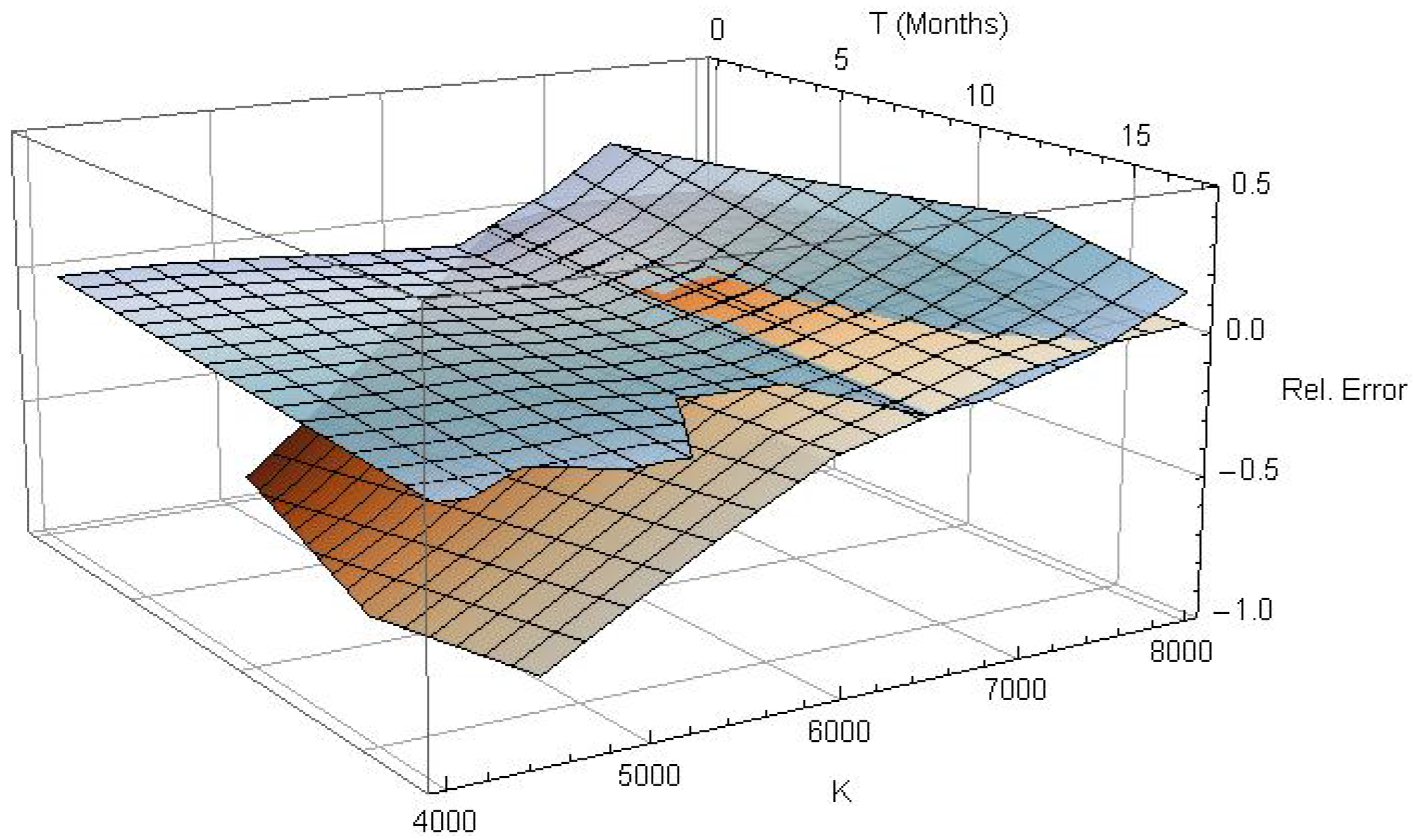
Figure 2.
Relative pricing error of European plain vanilla calls (blue) and puts (red) for , and .
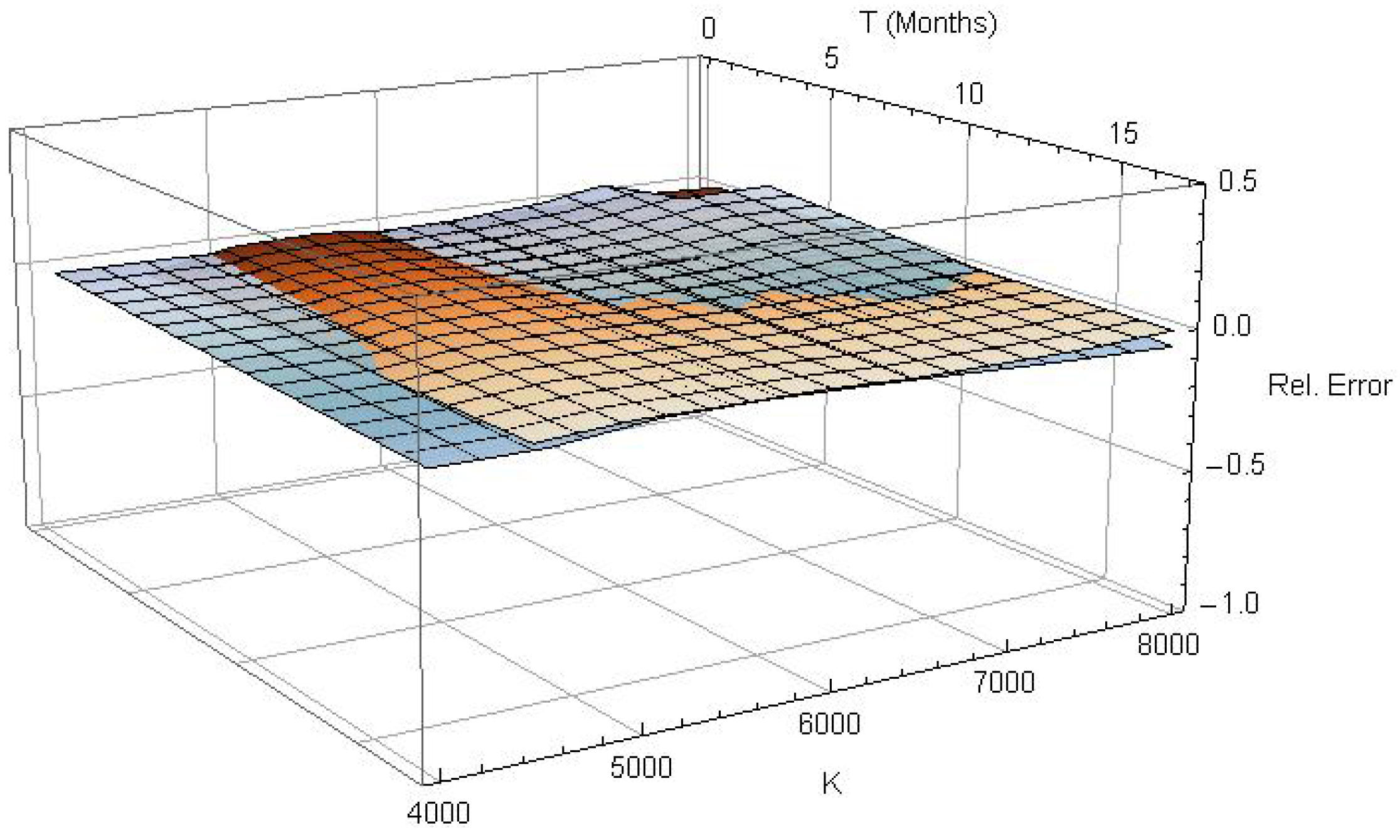
Figure 3.
Implied volatility surfaces—top left: linear interpolated data, top right: estimated (2,2)-model, bottom left: stochastic volatility inspired (SVI) parametrization, bottom right: SABR model.
Figure 3.
Implied volatility surfaces—top left: linear interpolated data, top right: estimated (2,2)-model, bottom left: stochastic volatility inspired (SVI) parametrization, bottom right: SABR model.
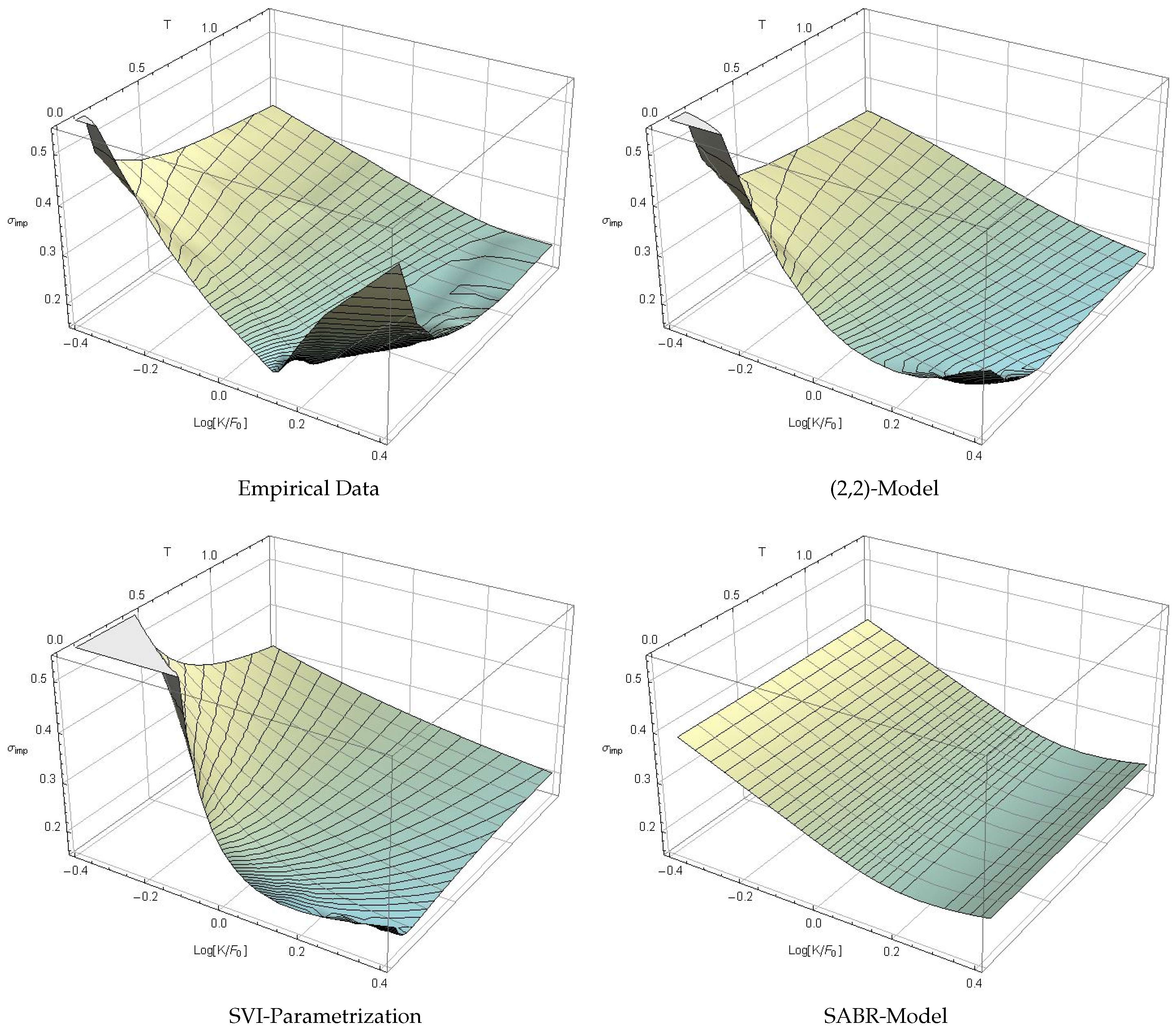
Figure 4.
Difference between observed implied volatility and conditional density (2,2)-model (top left), SVI parametrization (top right) and SABR model (bottom center).
Figure 4.
Difference between observed implied volatility and conditional density (2,2)-model (top left), SVI parametrization (top right) and SABR model (bottom center).

Figure 5.
Valuation of European vanilla capped calls (blue) and puts (red) with the Black–Scholes model (left) and (2,2)-model of conditional pricing density (right).
Figure 5.
Valuation of European vanilla capped calls (blue) and puts (red) with the Black–Scholes model (left) and (2,2)-model of conditional pricing density (right).
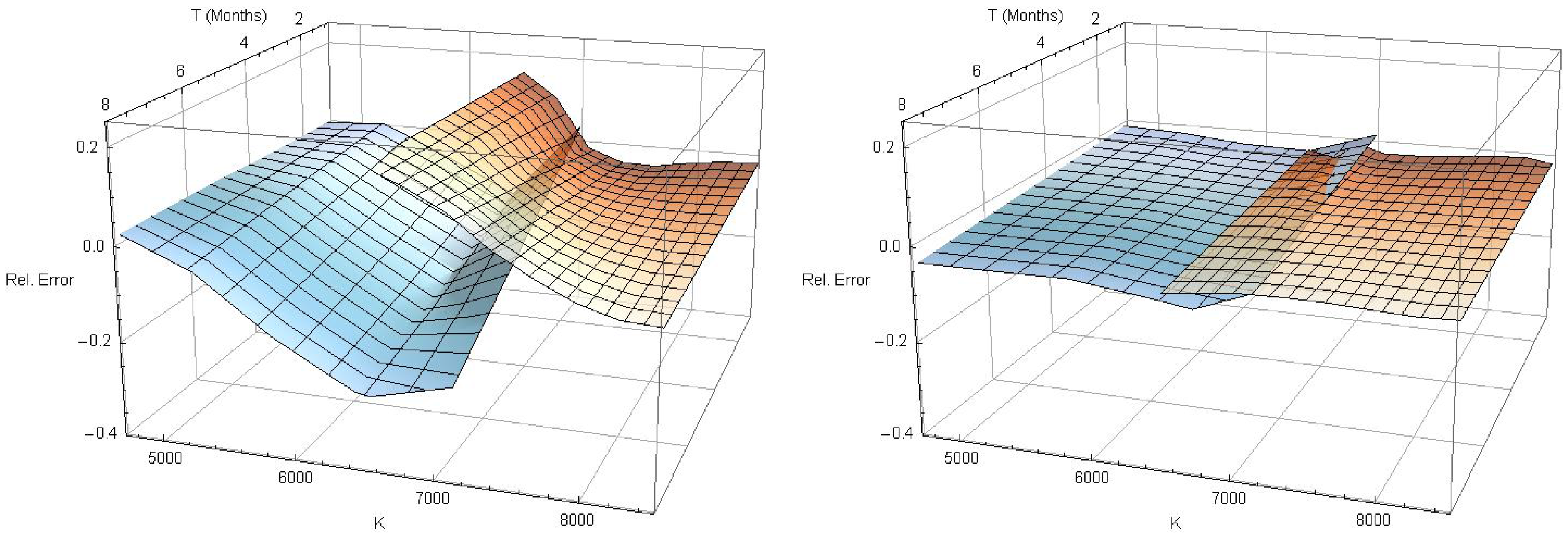
Figure 6.
One million draws from the multinomial density approximation for (left)—capped option valuation with 100,000 draws from importance distribution (right).
Figure 6.
One million draws from the multinomial density approximation for (left)—capped option valuation with 100,000 draws from importance distribution (right).

Table 1.
Model calibration for Fourier-coefficients. RMSE: root-mean-square error.
RMSE: 22.44% | RMSE: 20.02% | RMSE: 11.91% | RMSE: 11.42% | |
RMSE: 21.56% | RMSE: 15.52% | RMSE: 4.97% | RMSE: 1.66% | |
RMSE: 17.00% | RMSE: 15.51% | RMSE: 3.07% | RMSE: 1.43% | |
RMSE: 2.43% | RMSE: 2.42% | RMSE: 1.54% | RMSE: 1.47% | |
RMSE: 1.99% | RMSE: 1.73% | RMSE: 1.50% | RMSE: 1.16% | |
RMSE: 1.48% | RMSE: 1.67% | RMSE: 1.03% | RMSE: 1.09% |
Table 2.
RMSE of estimated implied volatility surfaces in the calibration sample (CS) and the full sample (FS).
Table 2.
RMSE of estimated implied volatility surfaces in the calibration sample (CS) and the full sample (FS).
| Model | Parameters | RMSE CS () | RMSE FS () |
|---|---|---|---|
| SVI | |||
| SABR | |||
© 2018 by the author. Licensee MDPI, Basel, Switzerland. This article is an open access article distributed under the terms and conditions of the Creative Commons Attribution (CC BY) license (http://creativecommons.org/licenses/by/4.0/).
Share and Cite
MDPI and ACS Style
Mazzoni, T. Asymptotic Expansion of Risk-Neutral Pricing Density. Int. J. Financial Stud. 2018, 6, 30. https://doi.org/10.3390/ijfs6010030
AMA Style
Mazzoni T. Asymptotic Expansion of Risk-Neutral Pricing Density. International Journal of Financial Studies. 2018; 6(1):30. https://doi.org/10.3390/ijfs6010030
Chicago/Turabian StyleMazzoni, Thomas. 2018. "Asymptotic Expansion of Risk-Neutral Pricing Density" International Journal of Financial Studies 6, no. 1: 30. https://doi.org/10.3390/ijfs6010030
Note that from the first issue of 2016, this journal uses article numbers instead of page numbers. See further details here.