Cross Hedging Stock Sector Risk with Index Futures by Considering the Global Equity Systematic Risk


1
Department of International Business Studies, National Chi Nan University, No.1, University Rd., Puli, Nantou 545, Taiwan
2
Department of Banking and Finance, National Chi Nan University, No.1, University Rd., Puli, Nantou 545, Taiwan
*
Author to whom correspondence should be addressed.
Int. J. Financial Stud. 2018, 6(2), 44; https://doi.org/10.3390/ijfs6020044
Submission received: 24 December 2017
/
Revised: 28 March 2018
/
Accepted: 10 April 2018
/
Published: 18 April 2018
(This article belongs to the Special Issue Finance, Financial Risk Management and their Applications)
Abstract
:This article investigates the effectiveness of TAIEX (Taiwan Stock Exchange) futures, Taiwan 50 futures, and nonfinance nonelectronics subindex (NFNE) futures for cross hedging the price risk of stock sector indices traded on the Taiwan stock exchange. A state-dependent volatility spillover GARCH hedging strategy is developed to capture the regime switching global equity volatility spillover effect. Empirical results show that the NFNE futures exhibit superior effectiveness as an instrument for hedging stock sector exposures compared with the TAIEX and Taiwan 50 futures. Simultaneous hedge using both NFNE and MSCI (Morgan Stanley Capital International) world index futures further improves the hedging effectiveness compared with the hedging strategy using only the NFNE futures. This shows the importance of hedging the global equity systematic risk of stock sectors by considering the comovement between domestic and global equity markets.
Keywords:
Markov regime switching; multiple futures hedging; volatility spillover; multivariate GARCH; cross hedgingJEL Classification:
C32; C51; G101. Introduction
It is well documented that the joint distribution of spot and futures returns is time varying. The implication of the time-varying joint distribution property for futures hedging is that in implementing an optimal futures hedging strategy, the hedger has to estimate the time-varying minimum variance hedge ratio (MVHR) (Baillie and Myers 1991; Kroner and Sultan 1993; Park and Switzer 1995). A considerable number of studies have been devoted to investigating futures hedging effectiveness by estimating the time-varying MVHR with a variety of multivariate GARCH (Generalized AutoRegressive Conditional Heteroskedasticity) models (Gagnon and Lypny 1998; Brooks et al. 2002; Byström 2003; Lafuente and Novales 2003; Lee and Yoder 2007a; Fernandez 2008; Choudhry 2009; Arouri et al. 2011; Chang et al. 2011; Pan et al. 2014; Cifarelli and Paladino 2015; Lai and Lien 2017; Park and Shi 2017; Sukcharoen and Leatham 2017). A general finding is that dynamic futures hedging is superior to conventional static hedging using constant MVHR.
Sarno and Valente (2000, 2005a, 2005b) found that the dynamic relationship between spot and futures returns may be characterized by regime shifts. To account for the changing market condition in implementing the optimal dynamic hedging strategy, a variety of regime switching GARCH models have been developed to estimate the regime switching time-varying MVHR (Lee and Yoder 2007a, 2007b; Alizadeh et al. 2008; Lee 2009a, 2009b, 2010; Lee and Tsang 2011; Sheu and Lee 2014; Dark 2015; Lai et al. 2017). In general, regime switching GARCH models exhibit superior hedging performance compared with their state-independent counterparts.
When hedging the price risk of a spot holding, hedgers normally apply the corresponding futures which are highly correlated with the underlying asset. When corresponding futures are not traded in the market, a closely related futures contract is required to implement the cross hedging strategy. For instance, Lee and Tsang (2011) considered a cross hedging strategy using American Depositary Receipts (ADRs) for hedging the price risk of individual stock. Adams and Gerner (2012) investigated the cross hedging performance of WTI (West Texas Intermediate), Brent, gasoil, and heating oil forwards to manage jet fuel spot price exposure. Ratner and Chiu (2013) examined the potential risk-reducing benefits of credit default swaps (CDS) against the price risk of the U.S. stock market sectors.
Taking into account the comovement between assets or markets might further improve futures hedging effectiveness. Fernandez (2008) analyzed a portfolio of metals traded on the London Metal Exchange and concluded that neglecting cross correlations leads to biased estimates of the optimal hedge ratios and the degree of hedging effectiveness. Lee and Tsang (2011) also found benefits of adding stock index futures in addition to ADRs for hedging single stock futures. Wu et al. (2011) investigated the volatility spillover effect from oil futures to corn spot and futures. They found that hedging performance is improved only marginally after adding additional crude oil futures to corn futures for hedging the corn spot exposure. The spillover model by Wu et al., however, does not account for the regime switching effect.
This paper investigates the performance of market index futures for the purpose of cross hedging the price risks of stock sector indices traded on the Taiwan stock exchange. Because there are no corresponding sector index futures for most of the sector indices traded on the Taiwan futures exchange, three domestic market indices futures—the TAIEX (Taiwan Stock Exchange) futures, the Taiwan 50 futures, and the nonfinance nonelectronics subindex (NFNE) futures—are applied to cross hedge the stock sector exposures. In this paper, we investigate the effectiveness of these futures as an instrument for cross hedging the price risk of stock sector holdings. Empirical results show that the NFNE futures exhibit superior hedging performance. We also consider simultaneous hedging using both NFNE and MSCI (Morgan Stanley Capital International) world index futures to hedge the domestic and global equity systematic risks of stock sectors with a regime switching volatility spillover GARCH (RSVSG) model.
The remainder of the article is organized as follows. The Markov regime switching volatility spillover GARCH (RSVSG) model is specified in Section 2. Section 3 presents the measurements of hedging performance, minimum variance hedge ratio (MVHR), and volatility spillover ratio. This is followed by discussions of data and empirical results. A conclusion ends the article.
2. Regime Switching Volatility Spillover GARCH (RSVSG) Model
This paper envisions a regime switching volatility spillover GARCH (RSVSG) model to hedge the price risk of stock sector holdings with both domestic and global stock index futures. RSVSG is an extension of the state-independent volatility spillover GARCH hedging model suggested by Wu et al. (2011) such that all system parameters are subject to regime shifting. The specification of RSVSG is given below:
Let denote a vector of returns with and being the stock sector index returns and domestic stock index futures returns, respectively. Without considering the volatility spillover from the global stock market to the domestic market,
where is a vector of state-dependent shocks, “” denotes transpose, and stands for the state variable assumed to follow a first-order two-state Markov process with logistic transition probabilities function given by
where and are unconstrained parameters to be estimated along with unknown system parameters via maximum likelihood estimation. and are state-dependent idiosyncratic shocks of stock sector index and domestic stock index futures, respectively. Specifically,
where is the information set available at time and is a state-dependent conditional covariance matrix assumed to have a bivariate diagonal regime switching BEKK (Baba–Engle–Kraft–Kroner) GARCH (Engle and Kroner 1995) specification (Lee and Yoder 2007a) given by
where , are the volatilities of stock sector index and domestic stock index futures returns, respectively, and is the covariance of stock sector index and domestic stock index futures returns. Let be the world stock index futures returns given by
where is the normalized state-dependent global stock shock and is the volatility of world stock index futures returns assumed to follow a regime switching GARCH(1,1) process:
When we consider the volatility spillover from the global stock market to the domestic stock sector index and domestic stock index futures markets, Equation (1) is modified to
where stands for the state-dependent shocks from the global market to domestic markets, specified as
and and are state-dependent volatility spillover parameters for the stock sector index and domestic stock index futures, respectively1. When we take into account both the effects of regime switching and global volatility spillover, Equations (2)–(9) constitute the specification of the regime switching volatility spillover GARCH (RSVSG). The variance and covariance dynamics in RSVSG are both state dependent and time varying and subject to the well-known path dependency problem. We follow the recombining procedures of Gray (1996) and Lee and Yoder (2007a) to solve the path dependency problem.
3. Measurements of Hedging Performance, Minimum Variance Hedge Ratio (MVHR), and Volatility Spillover Ratio
The hedging effectiveness is measured based on the percentage variance reductions of a hedging strategy over the unhedged position given by
where and are the variances of the hedged portfolio and the unhedged spot position, respectively. The return on hedged portfolio is equal to when the exposure on stock sector indices is hedged with only the domestic stock index futures and equal to when the exposure is hedged with both domestic stock index futures and world stock index futures. and are, respectively, the hedge ratios for domestic stock index futures and world stock index futures given by
where and are, respectively, the estimated conditional variances of domestic stock index futures and world stock index futures and , is the estimated conditional covariance of asset and asset .
We also compare the economic benefits of different hedging models using a mean–variance expected utility function (Kroner and Sultan 1993; Gagnon and Lypny 1998; Lee and Yoder 2007a, 2007b; Sheu and Lee 2014; Lai et al. 2017) given by
where is the coefficient of absolute risk aversion and stands for the expectation operator.
Because portfolio managers are usually more concerned about the variability of negative losses, the semivariance metric is employed to remove the effect of upside gains from the variance. Mathematically, this can be expressed as (Alizadeh et al. 2008)
where is the sample size and is the target return which is set to zero in order to distinguish between positive and negative realized portfolio returns. A short hedger is concerned about negative semivariance and a long hedger is concerned about positive semivariance.
According to Equations (8) and (9), under the assumption of no correlation between the normalized idiosyncratic shocks in domestic stock sector index and global stock index futures or between the normalized idiosyncratic shocks in domestic stock index futures and global stock index futures, the state-dependent conditional variances of domestic stock sector index and domestic stock index futures returns are given by
The state-dependent spillover ratio measures the proportion of the variances of domestic markets caused by the volatility spillover from global market shocks under different market regimes. The state-dependent volatility spillover ratios for domestic stock sector index and domestic stock index futures are respectively given by
Accordingly, the correlation between global stock index futures and domestic stock sector index and the correlation between global stock index futures and domestic stock index futures are respectively given by
4. Data Description and Empirical Results
The proposed regime switching volatility spillover GARCH (RSVSG) model was applied to the local contracts of TAIEX futures, Taiwan 50 futures, nonfinance nonelectronics subindex (NFNE) futures and global MSCI world index futures to hedge the spot exposure of Taiwan stock sector indices including textiles, communication and internet, transportation, retailing, automobiles, and plastics and chemicals. Spot and futures prices are Wednesday closing prices obtained from Datastream for the period from 20 May 2009 to 28 December 2016 to match the earliest available data for MSCI world index futures. All data are denominated in USD in line with the currency of global MSCI world index futures. Estimation of all models was conducted using data for up to 2015 (inclusive) and the remaining data were used for out-of-sample analysis. Returns of each price series were computed as the changes in the natural logarithms of prices multiplied by 100. We compared the hedging performance of the trivariate regime switching volatility spillover GARCH (RSVSG) model with those of the state-independent trivariate volatility spillover GARCH (VSG) and the state-independent bivariate BEKK GARCH, which does not account for the volatility spillover effect. We investigated whether simultaneous hedging by adding additional MSCI world index futures under regime switching improves futures hedging effectiveness.
Table 1 shows the summary statistics of spot and futures returns. Most of the unconditional mean returns are positive and quite small. The automobile industry has the largest unconditional mean return among all data investigated with a value of only 0.246%. The automobile industry, however, has the largest return volatility with a standard deviation of 3.867. According to the skewness, leptokurtosis, and significant Jarque–Bera statistics, the unconditional distributions of spot and futures returns are all asymmetric, fat-tailed, and non-Gaussian. This justifies the importance of modelling the spot and futures returns with more flexible regime switching GARCH models.
Table 2 shows the estimates of unknown parameters of the RSVSG using both NFNE and MSCI world index futures. and are the parameters of the logistic transition probabilities functions. Take textiles, for instance; the estimates of and are 2.829 and 1.954, respectively. According to Equations (2) and (3), the transition probability from low volatility state to high volatility state is 0.587 and the transition probability from high volatility state to low volatility state is 0.179. Figure 1 shows the regime probabilities of being in State 1. In the covariance equation, the persistence in volatility is measured with , and . For textiles, and are, respectively, 0.349 and 0.184, and and are, respectively, 0.745 and 0.045. The volatility persistence of textiles spot and NFNE futures is higher in the low volatility state (State 1). Figure 2 and Figure 3 show the state-dependent volatilities of textiles spot and NFNE futures, respectively. The average volatilities are, respectively, 2.020 and 3.781 for textiles spots in the low and high volatility states and are, respectively, 1.833 and 2.633 for NFNE futures in the low and high volatility states.
The spillover equation shows the parameter estimates of the volatility dynamic of MSCI world index futures and the spillover factors and . Figure 4 shows the state-dependent volatilities of MSCI world index futures. The average volatilities are equal to 1.862 and 2.92 in the low and high volatility states, respectively. The state-dependent volatility spillover ratios defined in Equations (16) and (17) measure the state-dependent proportion of the variances of domestic markets caused by the volatility spillover from global market shocks. The state-dependent spillover ratio is a function of spillover factors, the volatility of domestic market, and the volatility of MSCI world index futures. Figure 5 and Figure 6 show the state-dependent volatility spillover ratios of textiles spot and NFNE futures, respectively. The average volatility spillover ratios are, respectively, 0.409 and 0.275 for textiles spot in the low and high volatility states and are, respectively, 0.469 and 0.540 for NFNE futures in the low and high volatility states. The volatility spillover from the global market is higher in the NFNE futures than in the textiles spot for both regimes.
Table 3 shows the out-of-sample hedging effectiveness without considering the effects of regime switching and volatility spillover. We compare the hedging performance of TAIEX futures, Taiwan 50 futures, and NFNE futures with the hedging strategy implemented with the state-independent bivariate BEKK GARCH model. Taking the textiles sector, for instance, the variance of the unhedged spot position is 6.745. When hedging the spot exposures with TAIEX futures, Taiwan 50 futures, and NFNE futures, the variances on hedged portfolio returns are 2.983, 3.198, and 2.966 or variance reductions of 55.78%, 52.59%, and 56.03%, respectively. Hedging the spot exposure on the textiles sector with NFNE futures exhibits the highest variance reductions: the improvements are 0.25% and 3.44% compared with the TAIEX and Taiwan 50 futures, respectively.
Adopting NFNE futures for hedging the spot exposure creates the highest variance reductions for textiles, transportation, automobile, and plastics and chemicals sectors. The Taiwan 50 futures create the highest variance reductions for the retailing sector and the communication and internet sector, and the TAIEX futures show poor hedging effectiveness. Overall, we find that the NFNE futures perform better than the Taiwan 50 and TAIEX futures. We further calculate the utility gains of hedging with NFNE futures. The hedger is assumed to have an expected utility function given by Equation (12) with the coefficient of absolute risk aversion equal to 4 (Lee 2009a, 2009b, 2010; Sheu and Lee 2014; Lai et al. 2017)2. Taking the textiles sector, for example, the utility gains of NFNE futures are 0.075 and 0.963 compared with the TAIEX and Taiwan 50 futures, respectively. Again, the NFNE futures create the highest utility gains for the textiles, transportation, automobile, and plastics and chemicals sectors. This is consistent with the results of the variance reductions.
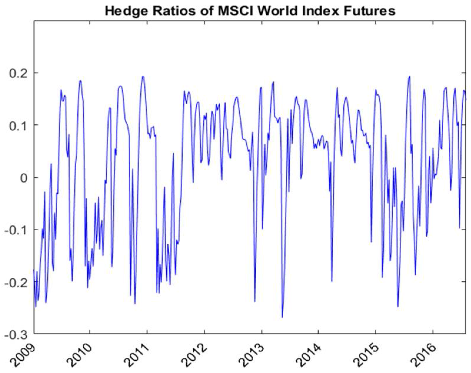
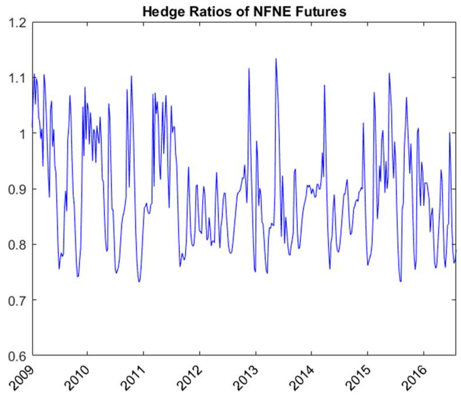
Table 4 shows the out-of-sample hedging effectiveness of RSVSG. RSVSG captures the effects of both global volatility spillover and regime switching and hedges the spot exposures using both NFNE and MSCI world index futures. Figure 7 and Figure 8 respectively show the hedge ratios of NFNE futures and MSCI world index futures for textiles estimated with RSVSG. Taking the textiles sector, for example, the variance of the unhedged spot position is equal to 6.745. When we apply the state-independent bivariate BEKK hedging strategy using only NFNE futures, the variance is 2.966—a variance reduction of 56.03%. If we take into account the volatility spillover effect from MSCI world index futures to domestic textiles sector and NFNE futures using a state-independent volatility spillover (VSG) model, the variance is 2.946—a variance reduction of 56.32%. Applying MSCI world index futures for hedging textiles spot exposure improves the hedging effectiveness. VSG is superior to BEKK for textiles, retailing, transportation, and communication and internet, but inferior to BEKK for automobiles and for plastics and chemicals. When we consider the effects of both volatility spillover and regime switching using both NFNE and MSCI world index futures, the variance of the hedged portfolio return by applying RSVSG is 2.930. The improvement by RSVSG in percentage variance reductions is 0.53% and 0.23% compared with the VSG and BEKK models, respectively. The incremental utility gains of RSVSG over VSG and BEKK are 0.135 and 0.053, respectively. Since most of the utility gains are positive for the data considered, hedging the stock sector exposure with additional MSCI world index futures under regime switching improves hedging effectiveness.
Because multiple futures hedging applies more futures contracts and is more costly to implement, we further investigate the superiority of RSVSG over BEKK and VSG by taking transaction costs into account. Taking textiles, for instance, if the hedger uses BEKK hedging, the average weekly utility is . With RSVSG hedging, the average weekly utility is . The hedger’s net benefit from using RSVSG hedging over BEKK hedging is equal to , where stands for the net average weekly transaction cost. If (in percentage) or 13.5 basis points, RSVSG hedging is preferred to BEKK hedging. Since the typical round trip transaction costs are around 0.03% (Lai et al. 2017), the net average weekly transaction cost between RSVSG and BEKK is defined as , where . Accordingly, the net average weekly transaction cost is equal to , or 0.223 basis points, which is smaller than 13.5 basis points. A mean–variance expected-utility-maximizing hedger would adopt RSVSG hedging even after taking account of the transaction costs. Similarly, the net average weekly transaction cost between RSVSG and VSG is equal to , or 0.189 basis points, which is smaller than 5.3 basis points, the net benefit from using RSVSG hedging over VSG hedging.
Table 5 presents the hedging effectiveness evaluated with semivariance reduction and semi-utility gain under regime switching and global volatility spillover effects. Negative and positive semivariance reflect the downside variation of hedged portfolio for short and long hedgers’ positions, respectively. Again, most of the incremental semi-utility gains of RSVSG over VSG and BEKK are positive. We reach the same conclusion that hedging the stock sector exposure with additional MSCI world index futures under regime switching improves hedging effectiveness.
5. Conclusions
There are two main questions investigated in this paper. First, because there are no corresponding sector futures for most sector indices traded on the Taiwan stock exchange, closely related futures must be applied for cross hedging the spot exposures on stock sectors. This article investigated the effectiveness of three potential futures as an instrument for cross hedging—TAIEX futures, Taiwan 50 futures, and NFNE futures. Second, since the domestic market is affected by global shocks and the shock spillover from the global market might depend on the state of market conditions, a regime switching volatility spillover GARCH hedging strategy was developed to investigate if simultaneous hedging using both domestic stock index futures and MSCI world index futures under regime switching increases hedging effectiveness.
Empirical results show that adopting NFNE futures for hedging the spot exposure creates the highest variance reductions for textiles, transportation, automobile, and plastics and chemicals sectors. TAIEX futures has the poorest hedging performance. Overall, we find that the NFNE futures perform better than the Taiwan 50 and TAIEX futures. Applying MSCI world index futures to capture the global stock systematic risk and hedging the spot exposures with both NFNE and MSCI world index futures improves hedging effectiveness. VSG is superior to BEKK for textiles, retailing, transportation, and communication and internet sectors. When we take into account the effects of both global volatility spillover and regime switching, the RSVSG hedging strategy exhibits superior hedging performance compared with the VSG and BEKK GARCH models. This shows the importance of hedging the stock sector price risks using both NFNE futures and MSCI world index futures implemented with a state-dependent volatility spillover model.
Acknowledgments
The authors would like to thank the anonymous referees and the editors for their useful comments. All remaining errors are ours.
Author Contributions
Wen-Chung Hsu is responsible for the data analysis and interpretation, critical revision of the article and final approval of the version to be published. Hsiang-Tai Lee is responsible for the theoretical framework design, data analysis and interpretation, drafting the article, and final approval of the version to be published.
Conflicts of Interest
The authors declare no conflict of interest.
References
- Adams, Zeno, and Mathias Gerner. 2012. Cross hedging jet-fuel price exposure. Energy Economics 34: 1301–9. [Google Scholar] [CrossRef]
- Alizadeh, Amir H., Nikos K. Nomikos, and Panos K. Pouliasis. 2008. A Markov regime switching approach for hedging energy commodities. Journal of Banking and Finance 32: 1970–83. [Google Scholar] [CrossRef]
- Arouri, Mohamed El Hedi, Jamel Jouini, and Duc Khuong Nguyen. 2011. Volatility Spillovers between Oil Prices and Stock Sector Returns: Implications for Portfolio Management. Journal of International Money and Finance 30: 1387–405. [Google Scholar] [CrossRef]
- Baillie, Richard T., and Robert J. Myers. 1991. Bivariate GARCH estimation of the optimal commodity futures hedge. Journal of Applied Econometrics 6: 109–24. [Google Scholar] [CrossRef]
- Brooks, Chris, Olan T. Henry, and Gita Persand. 2002. The Effect of Asymmetries on Optimal Hedge Ratios. Journal of Business 75: 333–52. [Google Scholar] [CrossRef]
- Byström, Hans NE. 2003. The Hedging Performance of Electricity Futures on the Nordic Power Exchange. Applied Economics 35: 1–11. [Google Scholar] [CrossRef]
- Chang, Chia-Lin, Michael McAleer, and Roengchai Tansuchat. 2011. Crude oil hedging strategies using dynamic multivariate GARCH. Energy Economics 33: 912–23. [Google Scholar] [CrossRef]
- Choudhry, Taufiq. 2009. Short-run deviations and time-varying hedge ratios: evidence from agricultural futures markets. International Review of Financial Analysis 18: 58–65. [Google Scholar] [CrossRef]
- Cifarelli, Giulio, and Giovanna Paladino. 2015. A Dynamic Model of Hedging and Speculation in the Commodity Futures Markets. Journal of Financial Markets 25: 1–15. [Google Scholar] [CrossRef]
- Dark, Jonathan. 2015. Futures hedging with Markov switching vector error correction FIEGARCH and FIAPARCH. Journal of Banking and Finance 61: 269–85. [Google Scholar] [CrossRef]
- Engle, Robert F., and Kenneth F. Kroner. 1995. Multivariate simultaneous generalized ARCH. Econometric Theory 11: 122–50. [Google Scholar] [CrossRef]
- Fernandez, Viviana. 2008. Multi-period hedge ratios for a multi-asset portfolio when accounting for returns co-movement. The Journal of Futures Markets 28: 182–207. [Google Scholar] [CrossRef]
- Gagnon, Louis, and Greg Lypny. 1998. Hedging short-term interest risk under time-varying distribution. The Journal of Futures Markets 15: 767–83. [Google Scholar] [CrossRef]
- Gray, Stephen F. 1996. Modeling the conditional distribution of interest rates as a regime-switching process. Journal of Financial Economics 42: 27–62. [Google Scholar] [CrossRef]
- Kroner, Kenneth F., and Jahangir Sultan. 1993. Time-varying distribution and dynamic hedging with foreign currency futures. Journal of Financial and Quantitative Analysis 28: 535–51. [Google Scholar] [CrossRef]
- Lafuente, Juan A., and Alfonso Novales. 2003. Optimal hedging under departures from the cost-of-carry valuation: Evidence from the Spanish stock index futures market. Journal of Banking and Finance 27: 1053–78. [Google Scholar] [CrossRef]
- Lai, Yu-Sheng, and Donald Lien. 2017. A Bivariate High-Frequency-Based Volatility Model for Optimal Futures Hedging. The Journal of Futures Markets 37: 913–29. [Google Scholar] [CrossRef]
- Lai, Yu-Sheng, Her-Jiun Sheu, and Hsiang-Tai Lee. 2017. A Multivariate Markov Regime-Switching High-Frequency-Based Volatility Model for Optimal Futures Hedging. The Journal of Futures Markets 37: 1124–40. [Google Scholar] [CrossRef]
- Lee, Hsiang-Tai. 2009a. Optimal futures hedging under jump switching dynamics. Journal of Empirical Finance 16: 446–56. [Google Scholar] [CrossRef]
- Lee, Hsiang-Tai. 2009b. A copula-based regime-switching GARCH model for optimal futures hedging. The Journal of Futures Markets 29: 946–72. [Google Scholar] [CrossRef]
- Lee, Hsiang-Tai. 2010. Regime switching correlation hedging. Journal of Banking and Finance 34: 2728–41. [Google Scholar] [CrossRef]
- Lee, Hsiang-Tai, and Wei-Lun Tsang. 2011. Cross hedging single stock with American Depositary Receipt and stock index futures. Finance Research Letters 8: 146–57. [Google Scholar] [CrossRef]
- Lee, Hsiang-Tai, and Jonathan K. Yoder. 2007a. A bivariate Markov regime switching GARCH approach to estimate the time varying minimum variance hedge ratio. Applied Economics 39: 1253–65. [Google Scholar] [CrossRef]
- Lee, Hsiang-Tai, and Jonathan Yoder. 2007b. Optimal hedging with a regime-switching time-varying correlation GARCH Model. The Journal of Futures Markets 27: 495–16. [Google Scholar] [CrossRef]
- Pan, Zhiyuan, Yudong Wang, and Li Yang. 2014. Hedging Crude Oil Using Refined Product: A Regime Switching Asymmetric DCC Approach. Energy Economics 46: 472–84. [Google Scholar] [CrossRef]
- Park, Jin Suk, and Yukun Shi. 2017. Hedging and speculative pressures and the transition of the spot-futures relationship in energy and metal markets. International Review of Financial Analysis 54: 176–91. [Google Scholar] [CrossRef]
- Park, Tae H., and Lorne N. Switzer. 1995. Bivariate GARCH Estimation of the Optimal Hedge Ratios for Stock Index Futures: A Note. The Journal of Futures Markets 15: 61–67. [Google Scholar] [CrossRef]
- Ratner, Mitchell, and Chih-Chieh Jason Chiu. 2013. Hedging stock sector risk with credit default swaps. International Review of Financial Analysis 30: 18–25. [Google Scholar] [CrossRef]
- Sarno, Lucio, and Giorgio Valente. 2000. The cost of carry model and regime shifts in stock index futures markets: An empirical investigation. The Journal of Futures Markets 20: 603–24. [Google Scholar] [CrossRef]
- Sarno, Lucio, and Giorgio Valente. 2005a. Empirical exchange rate models and currency risk: Some evidence from density forecasts. Journal of International Money and Finance 24: 363–85. [Google Scholar] [CrossRef]
- Sarno, Lucio, and Giorgio Valente. 2005b. Modelling and forecasting stock returns: Exploiting the futures market, regime shifts, and international spillovers. Journal of Applied Econometrics 20: 345–76. [Google Scholar] [CrossRef]
- Sheu, Her-Jiun, and Hsiang-Tai Lee. 2014. Optimal futures hedging under multi-chain Markov regime switching. The Journal of Futures Markets 34: 173–202. [Google Scholar] [CrossRef]
- Sukcharoen, Kunlapath, and David J. Leatham. 2017. Hedging downside risk of oil refineries: A vine copula approach. Energy Economics 66: 493–507. [Google Scholar] [CrossRef]
- Wu, Feng, Zhengfei Guan, and Robert J. Myers. 2011. Volatility spillover effects and cross hedging in corn and crude oil futures. The Journal of Futures Markets 31: 1052–75. [Google Scholar] [CrossRef]
| 1 | Because the state probability is time varying, and are also time varying after taking the weighted average using state probabilities. |
| 2 | Because all hedged portfolio returns are pretty small, the value of the expected utility is dominated by the second moment of the hedged portfolio return. Although it is not reported here, we find that hedging results are robust to the choice of the coefficient of absolute risk aversion for a wide range of (). A hedging strategy with lower volatility has higher expected utility regardless the choice of the coefficient of absolute risk aversion. |
Figure 1.
Regime probability of being in State 1 estimated with RSVSG for textiles.
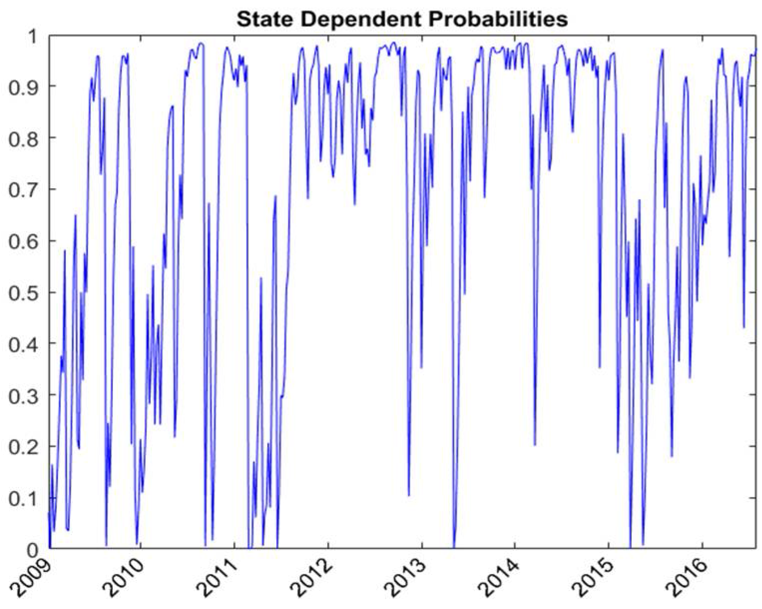
Figure 2.
State-dependent volatilities of textiles spot returns estimated with RSVSG.

Figure 3.
State-dependent volatilities of NFNE futures estimated with RSVSG for textiles.
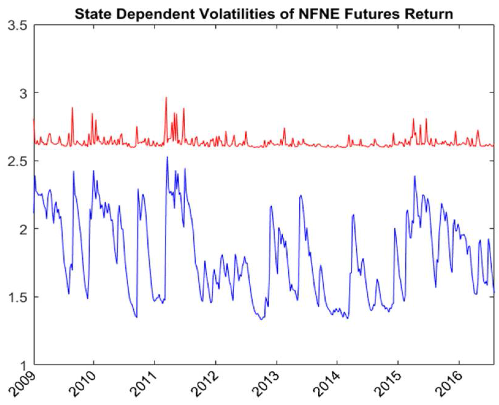
Figure 4.
State-dependent volatilities of MSCI world index futures estimated with RSVSG for textiles.
Figure 4.
State-dependent volatilities of MSCI world index futures estimated with RSVSG for textiles.
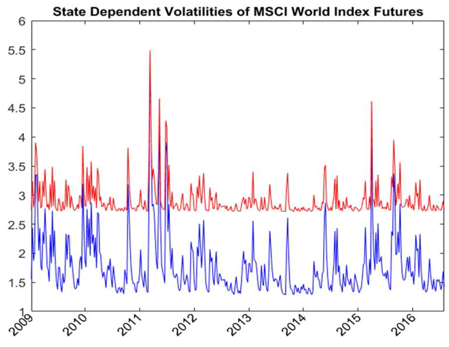
Figure 5.
The state-dependent volatility spillover ratios for textiles spot estimated with RSVSG.
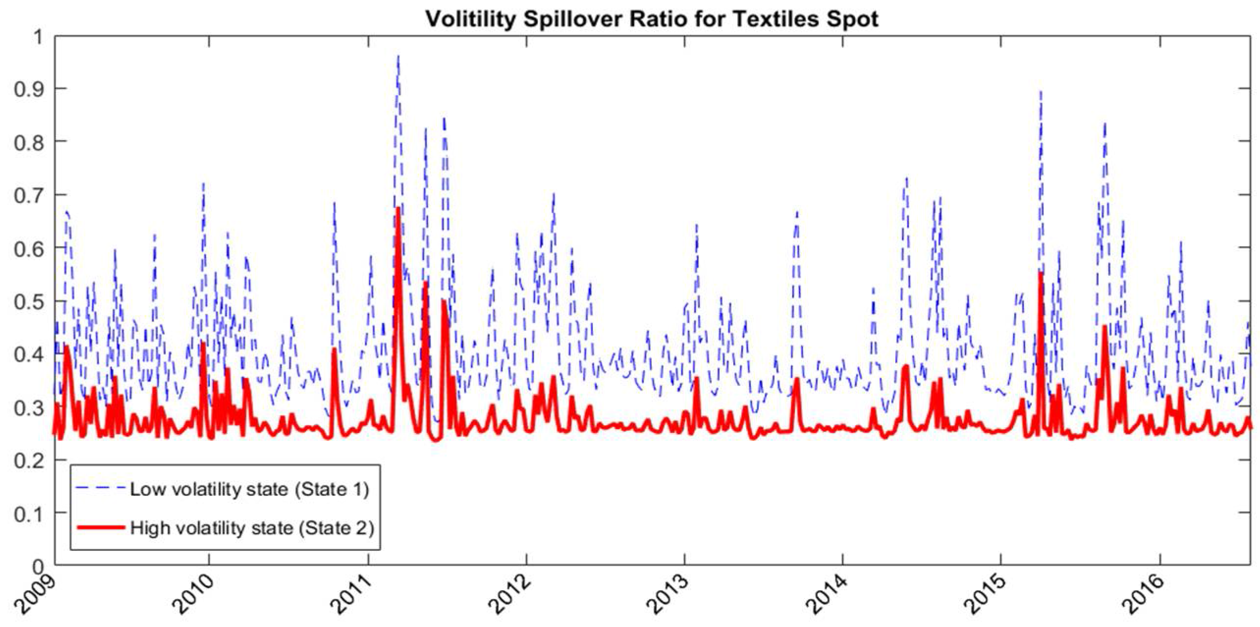
Figure 6.
The state-dependent volatility spillover ratios for NFNE futures estimated with RSVSG.
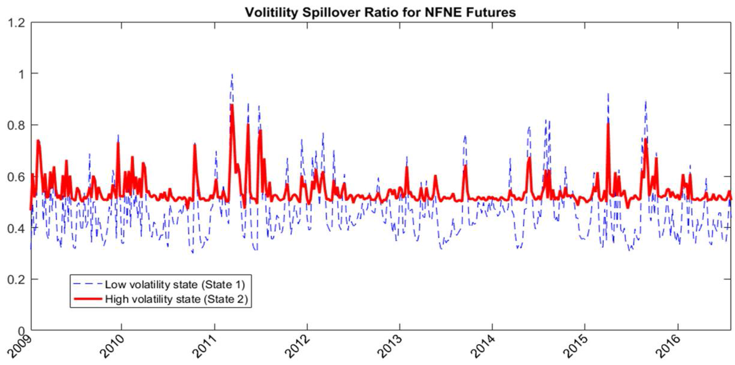
Figure 7.
Hedge ratios of NFNE futures estimated with RSVSG for textiles.

Figure 8.
Hedge ratios of MSCI world index futures estimated with RSVSG for textiles.

Table 1.
Summary statistics of weekly returns (in percentages).
| Textiles | Communication and Internet | Transportation | Retailing | |
|---|---|---|---|---|
| Mean | 0.086 | 0.028 | −0.111 | 0.147 |
| Maximum | 9.232 | 6.265 | 7.658 | 9.363 |
| Minimum | −11.979 | −8.869 | −11.430 | −11.416 |
| SD | 2.953 | 2.171 | 2.938 | 2.727 |
| Skewness | −0.478 | −0.414 | −0.437 | −0.317 |
| Kurtosis | 4.548 | 4.679 | 4.293 | 4.333 |
| Jarque–Bera | 54.808 *** | 57.960 *** | 40.306 *** | 36.042 *** |
| Automobile | Plastics and Chemicals | TAIFEX Futures | Taiwan 50 Futures | |
| Mean | 0.246 | 0.114 | 0.085 | 0.106 |
| Maximum | 12.810 | 8.512 | 6.392 | 6.540 |
| Minimum | −14.360 | −11.618 | −10.015 | −10.328 |
| SD | 3.867 | 2.786 | 2.560 | 2.588 |
| Skewness | −0.279 | −0.478 | −0.546 | −0.330 |
| Kurtosis | 3.940 | 4.605 | 3.897 | 3.493 |
| Jarque–Bera | 19.770 *** | 57.683 *** | 33.023 *** | 11.215 *** |
| Taiwan NFNE Futures | MSCI World Index Futures | |||
| Mean | 0.090 | 0.192 | ||
| Maximum | 7.668 | 7.941 | ||
| Minimum | −9.659 | −10.044 | ||
| SD | 2.579 | 2.173 | ||
| Skewness | −0.490 | −0.577 | ||
| Kurtosis | 4.113 | 5.134 | ||
| Jarque–Bera | 36.371 *** | 97.375 *** |
Note: *** indicates significance at the 1% level and returns (in percentage) are calculated as the differences in the logarithm of prices multiplied by 100. NFNE, MSCI, and TAIEX stand for nonfinance nonelectronics subindex, Morgan Stanley Capital International and Taiwan Stock Exchange, respectively.
Table 2.
Estimates of unknown parameters of the regime switching volatility spillover GARCH (RSVSG). Data estimation period is from 20 May 2009 to 30 December 2015.
Table 2.
Estimates of unknown parameters of the regime switching volatility spillover GARCH (RSVSG). Data estimation period is from 20 May 2009 to 30 December 2015.
| Textiles | Retailing | Transportation | Textiles | Retailing | Transportation | ||
|---|---|---|---|---|---|---|---|
| Transition Probability | Spillover Equation | ||||||
| 2.829 | 1.525 | 0.653 | 1.137 | 0.000 | 0.000 | ||
| (0.399) *** | (0.576) *** | (0.430) * | (0.463) *** | (0.041) | (0.083) | ||
| 1.954 | −0.352 | 1.332 | 0.240 | 0.270 | 0.166 | ||
| (0.566) *** | (0.453) | (0.468) *** | (0.098) *** | (0.126) ** | (0.082) *** | ||
| Covariance Equation | 0.242 | 0.544 | 0.379 | ||||
| 3 | −1.270 | 0.152 | 1.165 | (0.154) * | (0.085) *** | (0.094) *** | |
| (0.396) *** | (0.531) | (0.267) *** | 0.768 | 0.600 | 0.495 | ||
| 3.604 | 1.480 | 2.277 | (0.086) *** | (0.080) *** | (0.107) *** | ||
| (0.414) *** | (0.765) ** | (0.859) *** | 0.763 | 0.719 | 0.391 | ||
| −0.418 | 0.377 | 1.203 | (0.071) *** | (0.074) *** | (0.112) *** | ||
| (0.293) * | (0.282) * | (0.210) *** | 7.291 | 3.046 | 1.314 | ||
| 2.313 | 0.657 | 2.317 | (2.446) *** | (5.129) | (0.649) *** | ||
| (0.302) *** | (0.585) | (0.199) *** | 0.220 | 0.000 | 0.118 | ||
| 0.014 | 0.001 | −0.002 | (0.153) * | (0.039) | (0.086) * | ||
| (0.059) | (0.040) | (0.076) | 0.049 | 1.000 | 0.874 | ||
| 1.158 | 0.002 | 0.245 | (0.284) | (1.212) | (0.185) *** | ||
| (0.510) *** | (0.022) | (0.974) | 0.544 | 0.775 | 0.701 | ||
| 0.000 | 0.021 | 0.038 | (0.131) *** | (0.168) *** | (0.090) *** | ||
| (0.035) ** | (0.056) | (0.065) | 0.739 | 0.844 | 0.841 | ||
| −0.029 | −0.050 | 0.000 | (0.092) *** | (0.138) *** | (0.073) *** | ||
| (0.163) | (0.147) | (0.04) | |||||
| 0.000 | 0.080 | −0.076 | |||||
| (0.049) | (0.071) | (0.087) | |||||
| −0.145 | 0.066 | 0.000 | |||||
| (0.128) | (0.153) | (0.018) | |||||
| 0.591 | 0.781 | 0.236 | |||||
| (0.194) * | (0.075) *** | (0.210) | |||||
| 0.428 | 1.365 | −0.835 | |||||
| (0.269) *** | (0.155) *** | (0.332) *** | |||||
| 0.863 | 0.845 | −0.169 | |||||
| (0.050) * | (0.057) *** | (0.315) | |||||
| −0.156 | 1.286 | 0.091 | |||||
| (0.303) *** | (0.135) *** | (0.571) | |||||
| 2 | −1797.51 | −1781.97 | −1827.45 | ||||
| Communication and Internet | Automobile | Plastics and Chemicals | Communication and Internet | Automobile | Plastics and Chemicals | ||
| Transition Probability | Spillover Equation | ||||||
| 1.624 | 2.208 | 1.463 | 0.000 | 0.000 | 0.000 | ||
| (1.122) * | (0.829) *** | (0.485) *** | (0.050) | (0.080) | (0.076) | ||
| 0.001 | −0.013 | 0.026 | 0.234 | 0.196 | 0.279 | ||
| (0.036) | (0.098) | (0.202) | (0.114) ** | (0.224) | (0.198) * | ||
| Covariance Equation | 0.579 | 0.593 | 0.512 | ||||
| 3 | (0.564) | 0.163 | 0.711 | (0.188) *** | (0.147) *** | (0.102) *** | |
| (0.691) | (0.768) | (0.340) ** | 0.436 | 0.863 | 0.760 | ||
| 2.729 | 2.936 | 2.172 | (0.058) *** | (0.110) *** | (0.078) *** | ||
| (0.520) *** | (1.434) ** | (0.699) *** | 0.781 | 0.688 | 0.725 | ||
| 0.424 | 0.093 | 0.743 | (0.094) *** | (0.067) *** | (0.074) *** | ||
| (0.282) * | (0.514) | (0.475) * | 2.976 | 5.378 | 2.880 | ||
| 1.868 | 0.785 | 1.173 | (9.570) | (18.033) | (8.560) | ||
| (1.070) *** | (0.211) *** | (0.376) *** | 0.000 | 0.128 | 0.000 | ||
| −0.001 | 0.000 | 0.000 | (0.035) | (0.316) | (0.040) | ||
| (0.031) | (0.030) | (0.115) | 1.000 | 0.872 | 1.000 | ||
| 0.516 | 0.000 | 0.228 | (2.055) | (4.023) | (2.150) | ||
| (3.655) | (0.044) | (1.430) | 0.485 | 1.048 | 0.949 | ||
| −0.075 | 0.014 | 0.120 | (0.137) *** | (0.264) *** | (0.147) *** | ||
| (0.121) | (0.033) | (0.081) * | 0.727 | 0.897 | 0.794 | ||
| 0.485 | −0.010 | 0.185 | (0.204) *** | (0.116) *** | (0.122) *** | ||
| (0.273) ** | (0.104) | (0.121) * | |||||
| −0.130 | 0.063 | 0.072 | |||||
| (0.120) | (0.083) | (0.091) | |||||
| 0.153 | −0.129 | 0.098 | |||||
| (0.265) | (0.106) | (0.102) | |||||
| 0.662 | 0.853 | 0.699 | |||||
| (0.126) *** | (0.077) *** | (0.057) *** | |||||
| −0.395 | 1.278 | 0.990 | |||||
| (1.109) | (0.251) *** | (0.329) *** | |||||
| 0.805 | 0.956 | 0.760 | |||||
| (0.124) *** | (0.031) *** | (0.063) *** | |||||
| 0.948 | 1.089 | 1.162 | |||||
| (0.743) | (0.105) *** | (0.088) *** | |||||
| 2 | −1762.47 | −1933.01 | −1615.74 | ||||
1 Figures in parentheses are standard errors and *, **, and *** indicate significance at the 10% level, 5% level, and 1% level, respectively; 2 LL stands for the log likelihood value; 3 State 1 is the low volatility state.
Table 3.
Out-of-sample hedging effectiveness without regime switching and global volatility spillover effects estimated with bivariate BEKK GARCH model.
Table 3.
Out-of-sample hedging effectiveness without regime switching and global volatility spillover effects estimated with bivariate BEKK GARCH model.
| Variance of Hedged Portfolio Return | Percentage Variance Reduction 1 | Improvement of NFNE Futures over Other Futures 2 | Hedged Portfolio Returns | Expected Weekly Utility 3 | Utility Gain of NFNE Futures over Other Futures 4 | |
|---|---|---|---|---|---|---|
| Textiles | ||||||
| Unhedged | 6.745 | 0.086 | ||||
| TAIEX | 2.983 | 55.78% | 0.25% | −0.457 | −12.389 | 0.075 |
| Taiwan 50 | 3.198 | 52.59% | 3.44% | −0.485 | −13.277 | 0.963 |
| NFNE subindex | 2.966 | 56.03% | −0.450 | −12.314 | ||
| Retailing | ||||||
| Unhedged | 4.481 | 0.147 | ||||
| TAIEX | 2.457 | 45.17% | −2.46% | −0.104 | −9.932 | −0.451 |
| Taiwan 50 | 2.394 | 46.56% | −3.85% | −0.137 | −9.714 | −0.669 |
| NFNE subindex | 2.567 | 42.71% | −0.114 | −10.383 | ||
| Transportation | ||||||
| Unhedged | 5.132 | −0.111 | ||||
| TAIEX | 2.028 | 60.49% | 3.93% | −0.477 | −8.588 | 0.815 |
| Taiwan 50 | 2.127 | 58.56% | 5.86% | −0.517 | −9.025 | 1.252 |
| NFNE subindex | 1.826 | 64.42% | −0.468 | −7.773 | ||
| Communication and Internet | ||||||
| Unhedged | 3.166 | 0.028 | ||||
| TAIEX | 1.485 | 53.10% | −3.81% | 0.006 | −5.933 | −0.474 |
| Taiwan 50 | 1.238 | 60.91% | −11.62% | −0.035 | −4.985 | −1.422 |
| NFNE subindex | 1.606 | 49.29% | 0.016 | −6.407 | ||
| Automobile | ||||||
| Unhedged | 6.921 | 0.246 | ||||
| TAIEX | 2.026 | 70.73% | 2.34% | −0.394 | −8.497 | 0.672 |
| Taiwan 50 | 1.950 | 71.82% | 1.25% | −0.439 | −8.241 | 0.416 |
| NFNE subindex | 1.864 | 73.07% | −0.370 | −7.825 | ||
| Plastics and Chemicals | ||||||
| Unhedged | 4.404 | 0.114 | ||||
| TAIEX | 1.096 | 75.12% | 11.85% | 0.124 | −4.258 | 2.095 |
| Taiwan 50 | 1.054 | 76.06% | 10.91% | 0.068 | −4.150 | 1.987 |
| NFNE subindex | 0.574 | 86.97% | 0.133 | −2.163 | ||
Note: 1 Percentage variance reductions are calculated as the differences of the variance of unhedged position and the estimated variance of alterative models over the variance of unhedged position, multiplied by 100; 2 Improvement of NFNE futures over other futures is defined as the difference of the percentage variance reduction of hedging with NFNE futures and the percentage variance reduction of hedging with TAIEX futures and Taiwan 50 futures estimated with a bivariate BEKK GARCH model; 3 Expected weekly utility is calculated based on Equation (12); 4 Utility gain of NFNE futures over other futures is defined as the difference of the expected utilities of hedging with NFNE futures over the expected utilities of hedging with TAIEX futures and Taiwan 50 futures estimated with a bivariate BEKK GARCH model; 5 Estimation of all models was conducted using data from 20 May 2009 to 30 December 2015; the data from 6 January 2016 to 28 December 2016 were used for out-of-sample analysis.
Table 4.
Out-of-sample hedging effectiveness evaluated with variance reduction and utility gain under regime switching and global volatility spillover effects.
Table 4.
Out-of-sample hedging effectiveness evaluated with variance reduction and utility gain under regime switching and global volatility spillover effects.
| Variance of Hedged Portfolio Return | Percentage Variance Reduction 1 | Improvement of RSVSG over VSG and BEKK 2 | Hedged Portfolio Returns | Expected Weekly Utility 3 | Utility Gain of RSVSG over VSG and BEKK 4 | |
|---|---|---|---|---|---|---|
| Textiles | ||||||
| Unhedged | 6.745 | 0.086 | ||||
| BEKK | 2.966 | 56.03% | 0.53% | −0.450 | −12.314 | 0.135 |
| VSG | 2.946 | 56.32% | 0.23% | −0.448 | −12.233 | 0.053 |
| RSVSG | 2.930 | 56.56% | −0.458 | −12.180 | ||
| Retailing | ||||||
| Unhedged | 4.481 | 0.147 | ||||
| BEKK | 2.567 | 42.71% | 4.36% | −0.114 | −10.383 | 0.791 |
| VSG | 2.405 | 46.32% | 0.74% | −0.102 | −9.722 | 0.131 |
| RSVSG | 2.372 | 47.06% | −0.104 | −9.591 | ||
| Transportation | ||||||
| Unhedged | 5.132 | −0.111 | ||||
| BEKK | 1.826 | 64.42% | −0.43% | −0.468 | −7.773 | −0.094 |
| VSG | 1.800 | 64.93% | −0.95% | −0.466 | −7.664 | −0.203 |
| RSVSG | 1.849 | 63.98% | −0.473 | −7.867 | ||
| Communication and Internet | ||||||
| Unhedged | 3.166 | 0.028 | ||||
| BEKK | 1.606 | 49.29% | 2.05% | 0.016 | −6.407 | 0.244 |
| VSG | 1.554 | 50.93% | 0.40% | −0.005 | −6.220 | 0.057 |
| RSVSG | 1.541 | 51.33% | 0.001 | −6.162 | ||
| Automobile | ||||||
| Unhedged | 6.921 | 0.246 | ||||
| BEKK | 1.864 | 73.07% | 0.10% | −0.370 | −7.825 | 0.023 |
| VSG | 1.977 | 71.43% | 1.74% | −0.386 | −8.294 | 0.492 |
| RSVSG | 1.857 | 73.17% | −0.375 | −7.802 | ||
| Plastics and Chemicals | ||||||
| Unhedged | 4.404 | 0.114 | ||||
| BEKK | 0.574 | 86.97% | −1.64% | 0.133 | −2.163 | −0.300 |
| VSG | 0.710 | 83.88% | 1.44% | 0.106 | −2.733 | 0.270 |
| RSVSG | 0.646 | 85.32% | 0.123 | −2.463 | ||
Note: 1 Percentage variance reductions are calculated as the differences of the variance of unhedged position and the estimated variance of alterative models over the variance of unhedged position, multiplied by 100; 2 Improvement of RSVSG over VSG and BEKK is defined as the difference of the percentage variance reduction of hedging with RSVSG and the percentage variance reduction of hedging with VSG and BEKK; 3 Expected weekly utility is calculated based on Equation (12); 4 Utility gains of RSVSG over VSG and BEKK are defined as the differences of the expected utilities of hedging with RSVSG over the expected utilities of hedging with VSG and BEKK; 5 Estimation of all models was conducted using data from 20 May 2009 to 30 December 2015; data from 6 January 2016 to 28 December 2016 were used for out-of-sample analysis.
Table 5.
Out-of-sample hedging effectiveness evaluated with semivariance reduction and semi-utility gain under regime switching and global volatility spillover effects.
Table 5.
Out-of-sample hedging effectiveness evaluated with semivariance reduction and semi-utility gain under regime switching and global volatility spillover effects.
| Semivariance of Hedged Portfolio Return | Percentage Semivariance Reduction 1 | Improvement of RSVSG over VSG and BEKK 2 | Hedged Portfolio Returns | Expected Weekly Semi-Utility 3 | Semi-Utility Gain of RSVSG over VSG and BEKK 4 | |
|---|---|---|---|---|---|---|
| Textiles | ||||||
| Short hedgers‘ positions (negative semivariance) | ||||||
| Unhedged | 3.896 | 0.086 | ||||
| BEKK | 2.085 | 46.49% | 0.80% | −0.450 | −8.789 | 0.117 |
| VSG | 2.068 | 46.91% | 0.38% | −0.448 | −8.722 | 0.050 |
| RSVSG | 2.054 | 47.29% | −0.458 | −8.672 | ||
| Long hedgers‘ positions (positive semivariance) | ||||||
| Unhedged | 2.779 | 0.086 | ||||
| BEKK | 1.027 | 63.06% | 1.30% | −0.450 | −4.556 | 0.136 |
| VSG | 1.010 | 63.67% | 0.69% | −0.448 | −4.487 | 0.067 |
| RSVSG | 0.991 | 64.36% | −0.458 | −4.420 | ||
| Retailing | ||||||
| Short hedgers‘ positions (negative semivariance) | ||||||
| Unhedged | 2.135 | 0.147 | ||||
| BEKK | 1.323 | 38.05% | 7.26% | −0.114 | −5.404 | 0.630 |
| VSG | 1.181 | 44.69% | 0.62% | −0.102 | −4.826 | 0.052 |
| RSVSG | 1.168 | 45.31% | −0.104 | −4.774 | ||
| Long hedgers‘ positions (positive semivariance) | ||||||
| Unhedged | 2.265 | 0.147 | ||||
| BEKK | 1.208 | 46.66% | 1.71% | −0.114 | −4.947 | 0.165 |
| VSG | 1.174 | 48.18% | 0.20% | −0.102 | −4.798 | 0.016 |
| RSVSG | 1.169 | 48.38% | −0.104 | −4.781 | ||
| Transportation | ||||||
| Short hedgers‘ positions (negative semivariance) | ||||||
| Unhedged | 3.048 | −0.111 | ||||
| BEKK | 1.318 | 56.78% | 0.16% | −0.468 | −5.738 | 0.015 |
| VSG | 1.291 | 57.65% | −0.71% | −0.466 | −5.629 | −0.094 |
| RSVSG | 1.313 | 56.94% | −0.473 | −5.723 | ||
| Long hedgers‘ positions (positive semivariance) | ||||||
| Unhedged | 2.066 | −0.111 | ||||
| BEKK | 0.692 | 66.49% | 0.84% | −0.468 | −3.237 | 0.064 |
| VSG | 0.689 | 66.65% | 0.69% | −0.466 | −3.222 | 0.049 |
| RSVSG | 0.675 | 67.33% | −0.473 | −3.173 | ||
| Communication and Internet | ||||||
| Short hedgers‘ positions (negative semivariance) | ||||||
| Unhedged | 1.516 | 0.028 | ||||
| BEKK | 0.796 | 47.46% | 0.04% | 0.016 | −3.170 | −0.012 |
| VSG | 0.818 | 46.01% | 1.49% | −0.005 | −3.279 | 0.097 |
| RSVSG | 0.796 | 47.50% | 0.001 | −3.182 | ||
| Long hedgers‘ positions (positive semivariance) | ||||||
| Unhedged | 1.602 | 0.028 | ||||
| BEKK | 0.778 | 51.40% | 3.55% | 0.016 | −3.098 | 0.213 |
| VSG | 0.713 | 55.50% | −0.55% | −0.005 | −2.857 | −0.029 |
| RSVSG | 0.722 | 54.95% | 0.001 | −2.885 | ||
| Automobile | ||||||
| Short hedgers‘ positions (negative semivariance) | ||||||
| Unhedged | 4.012 | 0.246 | ||||
| BEKK | 1.323 | 67.01% | 2.33% | −0.370 | −5.664 | 0.370 |
| VSG | 1.412 | 64.81% | 4.54% | −0.386 | −6.033 | 0.739 |
| RSVSG | 1.230 | 69.34% | −0.375 | −5.294 | ||
| Long hedgers‘ positions (positive semivariance) | ||||||
| Unhedged | 2.794 | 0.246 | ||||
| BEKK | 0.642 | 77.04% | 0.68% | −0.370 | −2.936 | 0.072 |
| VSG | 0.694 | 75.16% | 2.57% | −0.386 | −3.162 | 0.298 |
| RSVSG | 0.622 | 77.72% | −0.375 | −2.865 | ||
| Plastics and Chemicals | ||||||
| Short hedgers‘ positions (negative semivariance) | ||||||
| Unhedged | 2.044 | 0.114 | ||||
| BEKK | 0.219 | 89.27% | 0.91% | 0.133 | −0.744 | 0.064 |
| VSG | 0.241 | 88.19% | 1.99% | 0.106 | −0.860 | 0.179 |
| RSVSG | 0.201 | 90.18% | 0.123 | −0.680 | ||
| Long hedgers‘ positions (positive semivariance) | ||||||
| Unhedged | 2.385 | 0.114 | ||||
| BEKK | 0.361 | 84.85% | −0.93% | 0.133 | −1.312 | −0.099 |
| VSG | 0.401 | 83.17% | 0.75% | 0.106 | −1.500 | 0.088 |
| RSVSG | 0.383 | 83.92% | 0.123 | −1.411 | ||
Note: 1 Percentage variance reductions are calculated as the differences of the variance of unhedged position and the estimated variance of alterative models over the variance of unhedged position, multiplied by 100; 2 Improvement of RSVSG over VSG and BEKK is defined as the difference of the percentage variance reduction of hedging with RSVSG and the percentage variance reduction of hedging with VSG and BEKK; 3 Expected weekly utility is calculated based on Equation (12); 4 Utility gains of RSVSG over VSG and BEKK are defined as the differences of the expected utilities of hedging with RSVSG over the expected utilities of hedging with VSG and BEKK; 5 Estimation of all models was conducted using data from 20 May 2009 to 30 December 2015; data from 6 January 2016 to 28 December 2016 were used for out-of-sample analysis.
© 2018 by the authors. Licensee MDPI, Basel, Switzerland. This article is an open access article distributed under the terms and conditions of the Creative Commons Attribution (CC BY) license (http://creativecommons.org/licenses/by/4.0/).
Share and Cite
MDPI and ACS Style
Hsu, W.-C.; Lee, H.-T. Cross Hedging Stock Sector Risk with Index Futures by Considering the Global Equity Systematic Risk. Int. J. Financial Stud. 2018, 6, 44. https://doi.org/10.3390/ijfs6020044
AMA Style
Hsu W-C, Lee H-T. Cross Hedging Stock Sector Risk with Index Futures by Considering the Global Equity Systematic Risk. International Journal of Financial Studies. 2018; 6(2):44. https://doi.org/10.3390/ijfs6020044
Chicago/Turabian StyleHsu, Wen-Chung, and Hsiang-Tai Lee. 2018. "Cross Hedging Stock Sector Risk with Index Futures by Considering the Global Equity Systematic Risk" International Journal of Financial Studies 6, no. 2: 44. https://doi.org/10.3390/ijfs6020044
Note that from the first issue of 2016, this journal uses article numbers instead of page numbers. See further details here.