Alpha Momentum and Price Momentum


Finance and Banking, Friedrich-Alexander-Universität Erlangen-Nürnberg, 90403 Nürnberg, Germany
*
Authors to whom correspondence should be addressed.
Int. J. Financial Stud. 2018, 6(2), 49; https://doi.org/10.3390/ijfs6020049
Submission received: 19 March 2018
/
Revised: 24 April 2018
/
Accepted: 1 May 2018
/
Published: 8 May 2018
Abstract
:We analyze a novel alpha momentum strategy that invests in stocks based on three-factor alphas which we estimate using daily returns. The empirical analysis for the U.S. and for Europe shows that (i) past alpha has power in predicting the cross-section of stock returns; (ii) alpha momentum exhibits less dynamic factor exposures than price momentum and (iii) alpha momentum dominates price momentum only in the U.S. Connecting both strategies to behavioral explanations, alpha momentum is more related to an underreaction to firm-specific news while price momentum is primarily driven by price overshooting due to momentum trading.
Keywords:
alpha momentum; price momentum; stock-specific return; price overshooting; slow information diffusion; reversalJEL Classification:
G11; G12; G141. Introduction
The price momentum effect is one of the most widely studied phenomena in financial research. Academic studies regularly analyze a common price momentum strategy which was first documented by Jegadeesh and Titman (1993). The basis of their strategy is the empirical finding that stocks with superior returns in the preceding months exhibit superior performance in subsequent months and vice versa. However, Grundy and Martin (2001) argue that the performance of price momentum depends strongly on the realizations of the underlying factors driving stock returns. To overcome this dependency, they implement a momentum strategy that ranks stocks on a stock-specific return component which they estimate based on monthly return data over the previous five years. Stock-specific momentum has also been documented by, e.g., Gutierrez and Prinsky (2007) and Blitz et al. (2011).
We contribute to this debate by introducing an innovative approach to implement a stock-specific momentum strategy relying on more short-term time frames using daily return data. In our empirical study, we first examine the relation between past alpha or past return and future returns in asset pricing tests. Our results indicate that past alpha (but not past return) has power in predicting the cross-section of individual stock returns in the U.S. In contrast, European results reveal that both past alpha and past return are related to future returns. We continue by studying the profitability of strategies based on both criteria in a portfolio context. Comparing our (daily three-factor) alpha momentum strategy with the common price momentum strategy, we find that alpha momentum is more profitable in the U.S. and exhibits less dynamic factor exposures and, therefore, is less volatile in both the U.S and in Europe. Finally, we find that alpha momentum dominates price momentum in the U.S. but that there is no clear dominance in Europe.
Apart from academic research showing the profitability of price momentum, there are several studies explaining this phenomenon. In the last decade, researchers have begun focusing on behavioral explanations. Such models assume that price momentum is due to an underreaction to firm-specific news or due to an overshooting effect caused by momentum trading. Among others, Barberis et al. (1998) and Hong and Stein (1999) show that investors tend to underreact to firm-specific news. Therefore, prices adjust slowly to this information and momentum can be identified. Chen and Lu (2017) confirm these results using options markets’ information. On the other hand, Hong and Stein (1999) also give evidence that stock prices can overshoot due to so-called momentum traders pushing prices of past winner stocks above, and of past loser stocks below, their fundamental value. Furthermore, Daniel et al. (1998) find evidence that investors become overconfident and drive stock prices away—with a time lag—from their fundamental value. These momentum profits are then reversed in the long run.
Our paper contributes to the literature by connecting alpha momentum and price momentum to these behavioral explanations. When we look at the long-term performance of both strategies, we find that alpha momentum does not reverse as strongly as price momentum. Our findings indicate that price momentum is predominately due to overshooting caused by momentum trading whereas alpha momentum can be more strongly related to underreaction to firm-specific news. Moreover, we find alpha momentum and price momentum to be sensitive to sentiment. Profits of both strategies are stronger following periods of optimistic sentiment which can be explained by overpriced loser stocks due to short-selling impediments (see Stambaugh et al. 2012) in the U.S. and by increased momentum trading in winner stocks in Europe.
Since Jegadeesh and Titman (1993) have documented the price momentum effect in the U.S., various studies analyzing the profitability of price momentum strategies in different countries and asset classes have been published. Among others, Rouwenhorst (1998); Dijk and Huibers (2002); Fama and French (2012); Leippold and Lohre (2012) and Asness et al. (2013) find evidence of stock momentum in countries worldwide. De Groot et al. (2012) document momentum to be significant for frontier markets. Moreover, Asness et al. (1997); Chan et al. (2000) and Bhojraj and Swaminathan (2006) show that momentum strategies based on country indices earn significant abnormal returns. Additionally, Moskowitz and Grinblatt (1999); Swinkels (2002); Scowcroft and Sefton (2005); Chen et al. (2012) and Szakmary and Zhou (2015) report the profitability of momentum strategies based on sector indices in different countries worldwide. Shleifer and Summers (1990) and Menkhoff et al. (2012) find evidence of momentum in currencies, Erb and Harvey (2006) and Gorton et al. (2013) in commodities. Asness et al. (2013) detect momentum, among other things, in global bond futures and Jostova et al. (2013) and Barth et al. (2018) in corporate bonds.
However, Blitz et al. (2011) show that momentum profits vanished in the U.S. after the stock market collapsed in 2000. In addition, Daniel and Moskowitz (2016) detect that price momentum strategies perform poorly after market declines and when market volatility is high. Their study is in line with Grundy and Martin (2001), who argue that price momentum strategies depend strongly on the performance of the underlying factor realizations driving stock returns. Accordingly, momentum strategies are often quite volatile and only perform well if factor realizations persist. To diminish the impact of these factors, Grundy and Martin (2001) implement a momentum strategy which does not rank stocks on raw returns but on stock-specific return components. Using five years of monthly return data, they apply a dummy variable approach and estimate a modified Fama and French (1993) alpha for a six-month formation period. Their momentum strategy buys stocks with high dummy alphas and sells stocks with low ones. They find this strategy to be less volatile than common price momentum strategies. Stock-specific momentum strategies have also been examined by Gutierrez and Prinsky (2007); Blitz et al. (2011); Chaves (2012) and Blitz et al. (2018a). In contrast to Grundy and Martin (2001), these studies do not rank stocks based on dummy alphas but on monthly residual returns. Van Zundert (2017) shows that volatility-adjusted momentum strategies exhibit lower crash risk and, therefore, higher Sharpe ratios. Similarly, Blitz et al. (2013) document higher and less volatile reversal returns for strategies based on the stock-specific component. Da et al. (2014) implement short-term reversal strategies that are corrected for Fama and French (1993) factors and cash-flow news. In summary, these studies analyzing stock-specific momentum or reversal strategies apply three to five years of monthly return data to estimate the factor exposures of stocks based on Fama and French (1993) regressions. Within this framework, the respective stock-specific component is calculated for a formation period which covers only one-, six- or twelve-monthly returns.
In our empirical analysis, we rank stocks on their stock-specific return component, similar to Grundy and Martin (2001). Unlike them, however, we estimate alpha by considering daily stock returns during the formation period only. In doing so, we run three-factor regressions based on a clearly higher number of return observations and estimate all regression parameters solely based on the return data during the formation period. Thus, possible differences between the factor exposures of stocks before and within the formation period do not impact our ranking. Finally, we do not need to restrict our sample to stocks with at least 36 months of return history and can therefore include recently issued stocks in our data sample.
Moreover, in contrast to Gutierrez and Prinsky (2007); Blitz et al. (2011); Chaves (2012) and Blitz et al. (2018a) we do not look at the residual returns of our regressions. As we use daily returns during the formation period, the mean residual return of our regressions is zero. Thus, all stock specific returns unexplained by the Fama-French model is included in our alpha.
We start our empirical analysis with asset pricing tests to examine whether past alpha and past return are related to future returns of individual stocks. Our results indicate that past alpha has power in predicting the cross-section of returns in the U.S. and in Europe. Then, we build zero-investment portfolios that buy recent winner and sell loser stocks according to past alpha or past return. Analyzing the performance of these momentum strategies, alpha momentum shows higher returns than price momentum in the U.S. Moreover, it exhibits less dynamic factor exposures within the investment period and is, therefore, less volatile in the U.S. and in Europe. The difference between both strategies can be attributed to time-dependent variations in the overlap between stocks in the zero-investment portfolios of our alpha momentum strategy and the price momentum strategy. This overlap decreases when factor-related return contributions have a relatively high impact on stock returns during the formation period. Finally, alpha momentum dominates price momentum in the U.S. whereas there is no such clear dominance in Europe.
Focusing on the long-term profitability of both strategies, our findings support behavioral explanations which assume that momentum is caused by an underreaction to new information and by an overshooting effect due to momentum trading. While we find evidence for both causes, the respective impact is different for alpha momentum and price momentum. First, the performance of a momentum strategy using a subset of stocks that are in the winner or loser decile based on their past return, but not based on their past alpha, reverses strongly in the U.S after a few months. Thus, this effect could be more strongly driven by these stocks overshooting due to momentum trading and a subsequent reversal. Nevertheless, we do not find these patterns in Europe. Second, when we look at a momentum strategy using only a subset of stocks that are in the winner or loser deciles based on their past alpha, but not based on their past return, we see that the performance of this strategy reverses only moderately in the U.S. while it actually becomes flat in Europe over 60 months. Thus, this pattern could be predominantly due to an underreaction to firm-specific news. Finally, a strategy that buys (sells) stocks that are concurrently in the winner (loser) deciles of both strategies outperforms in the first months but reverses in the long run in both the U.S. and in Europe. This effect could be due to an underreaction to firm-specific news in combination with overshooting due to momentum trading.
Finally, focusing on behavioral explanations for the momentum effect, we find both alpha momentum and price momentum to be sensitive to sentiment. Both strategies yield the highest risk-adjusted returns in optimistic periods in the U.S. as well as in Europe. In the U.S., these profits primarily arise due to the underperformance of loser stocks. This is in line with Stambaugh et al. (2012) who argue that especially these stocks are subject to mispricing in times of optimistic sentiment due to short-selling impediments. Moreover, our results also support Antoniou et al. (2013) who show that loser stocks are subject to cognitive dissonance in optimistic periods. In Europe, higher momentum profits in optimistic investment months could be due to increased momentum trading in winner stocks.
Portfolio Construction and Performance Evaluation
In our empirical analysis we focus on two momentum strategies: Common price momentum following Jegadeesh and Titman (1993) and our alpha momentum strategy. To begin with, we describe the construction of these strategies and the main differences between them.
A common price momentum strategy sorts stocks into deciles based on their past raw return during a J-month formation period (henceforth past return). For each stock i, this past return = (1 + ) is determined by cumulating the stock’s monthly raw returns over the formation months . The price momentum strategy consists of a zero-investment portfolio that buys stocks monthly in the highest decile and sells stocks monthly in the lowest decile. These stocks are held for K months, skipping one month between the formation period and the investment period to avoid possible short-term reversals (see, e.g., Jegadeesh 1990; Lehmann 1990). The common price momentum strategy is rebalanced every month.
According to the three-factor Fama and French (1993) model1, the return of stock i in excess of the risk-free return in month can be divided into different components:
where is the excess return on the market and and are the realizations of the size and value factors in month . According to Equation (1), the excess return of a stock can thus be decomposed into and , which are stock-specific, and a factor-related return contribution ().
By ranking stocks on their past return, the price momentum strategy depends strongly on time-dependent realizations of this factor-related return contribution during the formation period. For instance, if the market excess return is positive, price momentum strategies tend to buy high-beta stocks and to sell low-beta stocks. In general, these strategies remain profitable throughout the investment period, if market excess returns remain positive. However, if market conditions change between formation and investment period, price momentum strategies perform poorly.
To diminish the influence of factor realizations, similar to Grundy and Martin (2001), we implement our alpha momentum strategy by ranking stocks on their stock-specific component (alpha) during the formation period. However, to the best of our knowledge, we are the first to estimate alpha by considering daily stock returns only during the formation period. In doing so, we run three-factor regressions based on a clearly higher number of return observations and estimate all regression parameters solely based on the return data during the formation period. Thus, possible differences between the factor exposures of stocks before and within the formation period do not impact our ranking. Finally, we do not need to restrict our sample to stocks with at least 36 months of return history and can therefore include recently issued stocks in our data sample. In particular, at the end of each month t, we estimate the coefficients of the three-factor model for each stock i based on daily stock returns over the J-month formation period:
where is the return of stock i on day d in excess of the risk-free rate, is the market excess return and and are the daily realizations of the size and value factors on day d. To account for possible infrequent trading, we follow Dimson (1979) and include leaded and lagged factor returns in the Fama and French (1993) model to estimate the factor exposures.2 Our alpha momentum strategy buys stocks in the decile with the highest past daily three-factor alpha (henceforth past alpha) and sells stocks in the decile with the lowest past alpha.
To measure and compare the monthly performance of the common price momentum strategy and our alpha momentum strategy, we look at their average returns, Sharpe ratios, FF alphas and risk-adjusted returns during the evaluation period. To estimate the FF alphas of the momentum strategies, we first employ a Fama and French (1993) three-factor regression according to Equation (1) but use the return of the zero-investment portfolio in month t instead of the individual stock excess return . In doing so, this unconditional model assumes constant factor exposures over time.
Then, we measure risk-adjusted returns accounting for dynamic factor exposures. The literature presents different ways of measuring performance in this context. On the one hand, Grundy and Martin (2001) run Fama and French (1993) regressions using six monthly returns of the zero-investment portfolio subsequent to the time of investment to estimate the factor exposures of the momentum strategy. On the other hand, Daniel and Moskowitz (2016) use daily strategy returns over a two months period after investment to estimate the strategies’ factor exposures. There are two critics concerning this methodology. First, as factor loadings are estimated based on ex-post data, these factor loadings are not known by investors at the time of investment. Thus, they cannot be implemented in practice to hedge momentum strategies. However, Grundy and Martin (2001) show that these estimates are more accurate to measures risk-adjusted performance as factor loadings change between the formation and the investment period. On the contrary, Daniel and Moskowitz (2016) point out that hedged momentum returns are upward biased when using ex-post betas. Second, this approach implicitly assumes constant factor exposures of the momentum strategy during these estimation periods. However, the stock composition of momentum portfolios and thus factor exposures of the strategy change every month. Thus, Wang and Wu (2011) estimate the factor exposures based on monthly returns of individual stocks for each investment month t separately. First, they run monthly FF regressions for each stock over the past three years. They then use the betas of the stocks in the winner and loser deciles to determine average betas of the momentum strategy. In this way, they account for monthly-changing stock compositions and resulting time-dependent factor exposures. However, their factor estimates are based on data during and before the formation period and are thus do not represent the accurate factor exposures to measure risk-adjusted performance of momentum strategies. In our study, we therefore combine the advantages of both methodologies. Similar to Wang and Wu (2011), we determine factor exposures of the momentum strategy (, , ) in month t as the average factor exposures of the respective stocks in the momentum portfolios. Like Grundy and Martin (2001), we use six months beginning with the investment month t to estimate these factor exposures from month t to t + 5 but use daily return data. Based on this, the risk-adjusted return of the zero-investment momentum portfolio p in investment month t is calculated as:
2. Empirical Analysis
2.1. Data
Our study covers U.S. stock data from December 1981 to May 2014. Furthermore, we apply European stock data from December 1987 to May 2014, which is shorter for reasons of data availability.3 We construct our dataset using stock constituent lists from Thomson Reuters Datastream. All stock data is extracted in US dollars. The Appendix A explains in detail the construction of the dataset and the implementation of screening procedures following Ince and Porter (2006).
To implement our alpha momentum strategy and to measure the performance of price momentum and alpha momentum, we run Fama and French (1993) regressions using daily and monthly factor realizations. For the U.S., we extract these factors from the Kenneth R. French homepage.4 For Europe, we extract the factors from the AQR homepage, due to data availability.5
2.2. Return Predictability of Past Return and Past Alpha
Our empirical analysis starts by studying the determinants of future returns in the cross-section of individual stocks. We test whether stock returns are related either to past alpha or to past return by running Fama-MacBeth regressions. In particular, each month t, we run cross-sectional regressions explaining the future one-month, six-month or twelve-month stock returns with the past twelve-month return from t − 13 to t − 2 (model 1), the past alpha estimated from t − 13 to t − 2 (model 2) or with both variables (model 3). In our cross-sectional regressions, we control for various stock characteristics commonly used in this context. We include control variables for size (log(ME)) and book-to-equity-market-ratio (log(BE/ME)) according to Fama and French (1992) and past return in month t − 1 following Novy-Marx (2013). Like in Gutierrez and Kelley (2008) and Loughran and Wellman (2011), size is measured as the market value of stocks in June of year t. Furthermore, book-to-market equity is calculated as the book value in fiscal year t − 1 divided by the market value in December of year t − 1. Similar to Novy-Marx (2013), we exclude financial firms and trim independent variables at the 1% and 99% levels. After running monthly cross-sectional regressions, we calculate average factor exposures of the time series of each coefficient.
For the U.S., Panel A of Table 1 shows that the past twelve-month return has no impact on future returns of individual stocks over the evaluation period from 1984 to 2013 (Model 1). Coefficients on the past twelve-month returns are insignificant for all three future return intervals. On the other hand, factor exposures on past alphas are significant at the 1%-level for the one-month future return (Model 2). Nevertheless, the significance of past alpha in the cross-section of returns vanishes when we look at longer future return intervals. Finally, when we include both past return and past alpha in our cross-sectional regressions (Model 3), the factor exposures of past alpha stay positive and significant at least at the 10%-level for all future return intervals. On the other hand, coefficients on past return remain insignificant.
For Europe, Panel B of Table 1 reveals that the past return is significantly related to the one-month future return over the evaluation period from 1990 to 2013 (Model 1). However, the coefficient on the past return becomes insignificant for longer future return intervals. On the other hand, the coefficient on past twelve-month alpha is significant for all future return intervals (Model 2). Including both past return and past alpha into our regression (Model 3), we find that only past return has a significant impact on the one-month return. However, for longer return intervals we see that the coefficient on past return becomes insignificant while that of past alpha stays positive and becomes significant.
In summary, our monthly regressions reveal that especially past alpha has power in predicting the cross-section of returns in the U.S. In Europe, both past return and past alpha are related to the cross-section of future returns. We thus assume that momentum strategies based on past alpha should in each case generate positive abnormal returns.
2.3. Performance of Momentum Strategies in Portfolio Context
In this section, we analyze the performance of zero-investment portfolios based on past return and past alpha. For the sake of brevity, we focus on the following two selected momentum strategies. Both define stocks in the winner decile and in the loser decile based on a twelve-month formation period (J12). We skip a month after formation to account for short-term reversal effects. Since the impact of past return and past alpha decreases in the cross-section of returns for longer future return intervals, we concentrate on momentum strategies with a one- and with a six-month investment period (K1, K6). Moreover, especially these J12/K1 and J12/K6 strategies are broadly used in the empirical literature.6 The K6 strategies consist of six overlapping cohorts which are constructed based on the past return (past alpha) at the end of month t and in the previous five months.
Panel A of Table 2 shows for the full evaluation period in the U.S., that alpha momentum exhibits higher average returns, higher Sharpe ratios, higher FF alphas and higher risk-adjusted returns. Testing the statistical difference between alpha momentum and price momentum based on mean returns, we do not find these differences to be statistically different from zero.7 However, when looking at the economic significance between the strategies, we find mean returns of alpha momentum to be significantly higher, with return differences up to 37 bps per month (J12/K6). Thus, an investor would have achieved up to 4.44% higher returns per year by investing in alpha momentum. Focusing at ten-year sub-periods, alpha momentum returns are higher than price momentum returns from 1994 onwards. However, both effects disappear in the U.S. during the most recent sub-period.
We find different patterns for our European sample in Panel B. Common price momentum strategies mostly exhibit economically (but not statistically) higher average returns, higher FF alphas and risk-adjusted returns over the full evaluation period and in both ten-year sub-periods. Nevertheless, due to a lower return volatility, the Sharpe ratios of alpha momentum are higher than those of the common price momentum strategy over the full evaluation period and especially in the most recent ten-year sub-period.
Comparing the results from the U.S. to those from Europe, we find momentum returns to be lower in the U.S. which might be due to faster information diffusion. Looking at mean returns, these differences are mostly statistically significant. Trading strategies based on past return are often applied in the U.S., as is well known since the seminal paper of Jegadeesh and Titman (1993).
To analyze differences between alpha momentum and price momentum in detail, we now look at the intersection of stocks in the zero-investment-portfolios of both strategies to see whether this overlap varies over time. Figure 1 plots all price momentum winner (loser) stocks with respect to their position in alpha momentum deciles. For instance, the “10.α-decile” (“1.α-decile”) area shows the percentage of all price momentum winner (loser) stocks that are also alpha momentum winner (loser) stocks. Therefore, this area shows a time-dependent overlap between price momentum and alpha momentum stocks. The “9.α-decile” (“2.α-decile”) area presents the percentage of all price momentum winner (loser) stocks that are in the ninth (second) decile when we rank according to past alpha, and so on. Obviously, the number of overlapping stocks between price momentum and alpha momentum varies over time. For winner and loser stocks, on average, the overlap is approximately 59% for the U.S. (Panel A) and 62% for Europe (Panel B). Comparing price momentum winner stocks with price momentum loser stocks, we find that loser stocks are more often located in more deviating alpha momentum deciles. In addition, each plot of Figure 1 shows a line presenting the negative absolute difference between the average monthly factor-related return contribution of price momentum and alpha momentum for the winner (loser) stocks. As expected, the overlap between alpha momentum and price momentum varies most when the absolute difference between the average factor-related return contributions is large.
To sum up, our findings reveal differences in the performance and in the stock composition between alpha momentum and price momentum. Moreover, these differences are clearly related to variations in the factor-related return contributions.
2.4. Dynamic Factor Exposures of Momentum Strategies
In this section, we test whether the factor exposures of alpha momentum and price momentum are stable or if they change over time. In context with price momentum strategies, the ranking of stocks is influenced by realizations of the underlying factors driving stock returns. For instance, if the market excess return is positive during the formation period, price momentum strategies favor buying high-beta stocks and selling low-beta stocks and vice versa. As factor realizations vary over time, resulting factor exposures of price momentum also change. Therefore, the Fama and French (1993) model, which assumes constant factor exposures, cannot sufficiently identify the risk of such momentum strategies. In terms of variance, only up to 8.71% (10.57%) of the return variation of the price momentum strategy can be explained by this unconditional model in the U.S. (Europe). Alpha momentum should be less dependent on changes in factor realizations, because it sorts stocks on their past alpha only. Accordingly, the explanatory power of the Fama and French (1993) model is higher for our alpha momentum strategy by up to 20.81% (11.29%) for the U.S. (Europe).
Following Gutierrez and Prinsky (2007) and Wang and Wu (2011), we account for time-varying factor exposures of price momentum and alpha momentum when measuring risk-adjusted returns. Figure 2 shows the average factor exposures over time of price momentum and alpha momentum estimated based on daily returns of individual stocks. Obviously, the factor exposures of the two strategies vary strongly, both in the U.S. (Panel A) and Europe (Panel B). Thus, even ranking stocks on their past alpha leads to a strategy with time-varying factor exposures. Nevertheless, the volatility of the factor exposures of price momentum is higher than that of alpha momentum.
As described in Section 2, when determining risk-adjusted returns, we hedge out the factor exposures for each investment month separately. In doing so, this dynamic hedging strategy explains up to 49.90% (41.69%) of the variance of the price momentum strategy and up to 43.58% (23.31%) of the alpha momentum strategy in the U.S. (Europe). Hence, this time-varying approach better explains the return variations of both strategies. Notably, even after hedging out the factor exposures of price momentum and alpha momentum, both strategies generate differing positive risk-adjusted returns during the full evaluation period and most ten-year sub-periods (see Table 2).
2.5. Dominance of Momentum Strategies
In this section, we analyze whether price momentum dominates alpha momentum, or the other way around, by running two tests following George and Hwang (2004). We first apply pairwise nested comparisons examining the performance of strategies based on past alpha, conditional on the ranking according to past return, and vice versa. The left part of Table 3 contains the results, where we first assign stocks to quintile portfolios according to past return and then further rank each quintile on past alpha. In each past return quintile, alpha momentum is determined as the difference between the respective winner and loser quintile based on past alpha (A5–A1). The right part of Table 3 reports results, where stocks are sorted first according to past alpha and then further divided into quintiles according to past return. In each past alpha quintile, price momentum is determined as the difference between the respective winner and loser quintiles based on past return (P5–P1).
For the U.S. (Panel A), we find positive and significant risk-adjusted returns for alpha momentum in past return quintiles. However, within past alpha quintiles, the profitability of price momentum disappears. We find different results for Europe (Panel B). Here, both alpha and price momentum yield significant profits within most of the conditionally ranked quintiles, though price momentum profits in past alpha quintiles are somewhat stronger.
To rule out that these findings are mainly driven by rankings on more extreme past returns (alphas), we also double-sort stocks according to the same criterion (Bandarchuk and Hilscher 2013). For the U.S., Panel A of Table 4 reveals that it is not possible to realize positive and significant price momentum profits within past return quintiles. We find similar results for alpha momentum in past alpha quintiles. Momentum profits are low within most quintiles. In Europe (Panel B), double-sorting according to both criteria leads to positive and significant momentum profits.
In summary, our findings reveal that alpha momentum strategies are more promising in predicting future performance and dominate price momentum in the U.S., while there is no clear dominance of one strategy in Europe. The difference between the U.S. and Europe could be explained by the clearly stronger price momentum and alpha momentum effect in Europe. That is why double-sorting leads to significant profits according to both criterions and why there is no clear dominance of one strategy in Europe.
To test the robustness of the previous dominance results, we now determine the profitability of a single strategy independent of the other by explaining the one-month future return of individual stocks by a cross-sectional regression approach similar to the one used in Section 2.3. However, in contrast, we focus here on stocks that are in the winner or loser deciles only. Thus, our dependent variables are four dummy variables indicating whether stock i is part of the winner or loser decile according to past return or past alpha in month t. For the J12/K1 strategy, we implement one cross-sectional regression for the one cohort held in each investment month. The J12/K6 strategy, however, consists of six overlapping cohorts each month. Thus, following George and Hwang (2004), we run one cross-sectional regression for each of the six cohorts held in month t. Within these cross-sectional regressions, the dummy variables change regarding the stock composition in the respective winner or loser deciles of the six overlapping cohorts. More precisely, the dummy variables of a cross-sectional regression are set to one if a stock is ranked in the winner or loser deciles in the respective cohort. Moreover, we control for market capitalization (log(ME)) and the past return in month t − 1 to get results comparable to George and Hwang (2004).8
After running these monthly cross-sectional regressions, we first calculate average exposures on the dummy variables for the J12/K6 strategy over the six different cross-sectional regressions in each investment month t, one for each cohort. Then, time-series averages of all coefficients are measured.
Results in Table 5 confirm previous findings from the nested pairwise comparison. In the U.S. (Panel A), alpha momentum dominates price momentum. Differences in the coefficients between the winner and loser deciles of alpha momentum (A10–A1) are highly significant for J12/K1 and J12/K6. On the other hand, for price momentum these differences (P10–P1) are insignificant. For Europe, Panel B reveals that the respective differences for price momentum are higher than those for alpha momentum. However, the differences for alpha momentum stay positive and significant for J12/K1 and J12/K6. This indicates that both alpha momentum and price momentum are profitable in addition to the other strategy.
Comparing U.S. and European results, the cross-sectional test reveals that price momentum profits are low and not significant in the U.S. On the other hand, we find highly significant price momentum profits in Europe. When we look at alpha momentum, we find comparable positive and significant profits for both the U.S. and for Europe.
3. Sources of Different Momentum Profits
3.1. Momentum Effects for Subsets of Stocks and Long-Term Performance
Our empirical findings in Section 2.3 show that the unconditional as well as the conditional Fama and French (1993) framework cannot fully explain the profits of alpha momentum and price momentum. Both strategies exhibit positive and significant FF alphas and risk-adjusted returns in the U.S. and in Europe based on the full evaluation period. Thus, we now ask whether behavioral causes can explain these momentum phenomena.
Behavioral explanations assume that momentum is driven by an underreaction to firm-specific news or by overshooting caused by momentum trading. Among others, Barberis et al. (1998) and Hong and Stein (1999) postulate that some investors tend to underreact to firm-specific news. Therefore, prices adjust slowly to this new information and momentum can be identified. Chen and Lu (2017) confirm these results using options markets’ information. On the other hand, Hong and Stein (1999) presume that stock prices can overshoot because so-called momentum traders do not trade based on fundamental information but on past price changes only. These investors push prices of past winner (loser) stocks above (below) their fundamental value in the short run. Resulting momentum profits are then reversed in the long run. Furthermore, Daniel et al. (1998) argue that investors become overconfident about their trading abilities and drive stock prices away from their fundamental value. In their seminal paper, De Bondt and Thaler (1985) find that past loser stocks outperform past winner stocks over three to five years. Lee and Swaminathan (2000) and Jegadeesh and Titman (2001) also document reversed momentum strategies in the long run.
In the following, we explore to what extent alpha momentum and price momentum are related to these behavioral explanations. We therefore follow the methodology of Gutierrez and Prinsky (2007). In a first step, we construct three subset portfolios to distinguish between winner or loser stocks according to past price only, according to past alpha only or according to both criteria at the same time. We then first compare the performance of these subset portfolios in the short run. In a second step, we analyze the long-term performance of alpha momentum, price momentum and the three subset portfolios.
To begin with, similar to Gutierrez and Prinsky (2007), we identify three different types of momentum stocks by comparing the stocks in the winner and loser deciles according to both past price and past alpha. First, we focus on stocks that are in the winner and loser deciles according to past return, but not in the respective deciles based on past alpha. Accordingly, this “Price ∉ Alpha” momentum strategy buys (sells) the subset of stocks that are in the winner (loser) decile based on their past return, but not based on their past alpha. Second, the “Alpha ∉ Price” momentum strategy consists of a zero-investment portfolio of stocks that are winner or loser stocks based on their past alpha, but not on their past return. Third, the “Price Alpha” momentum portfolio contains stocks that are in the winner (loser) deciles based on both past return and past alpha at the same time.
For the U.S., Panel A of Table 6 presents the performance of these subset strategies. For the full evaluation period, “Price ∉ Alpha” yields lower average returns, Sharpe ratios, FF alphas and risk-adjusted returns than “Alpha ∉ Price” and “Price Alpha” for J12/K1 and J12/K6. Return differences are economically significant; with up to 7.5% p.a. The results differ within the sub-periods. For the first sub-period, we find similar results to Gutierrez and Prinsky (2007). “Price Alpha” and “Price ∉ Alpha” exhibit higher returns than the “Alpha ∉ Price”. In the second and third sub-period, “Alpha ∉ Price” remains profitable, while the returns of the other strategies decrease. Considering the most recent ten-year sub-period from January 2004 to December 2013, the performance of “Price ∉ Alpha” momentum and “Price Alpha” momentum turns negative and insignificantly in terms of FF alphas and risk-adjusted returns for J12/K1 and J12/K6. Only “Alpha ∉ Price” momentum produces positive and significant results at the 5% level for these performance measures.
Overall, these results support behavioral explanations for the momentum effect. First, “Price ∉ Alpha” momentum could be predominately driven by prices overshooting due to momentum trading since an underreaction to firm-specific news should be firm-specific and thus should also be reflected in alpha. We find “Price ∉ Alpha” to be profitable during the first ten-year sub-period. Nevertheless, this profitability vanishes during the second ten-year sub-period after Jegadeesh and Titman published their seminal paper in 1993. Second, “Alpha ∉ Price” profits are positive and highly significant for the full evaluation period and for all ten-year sub-periods. This could be mainly driven by an underreaction to firm-specific news since momentum traders do not tend to invest in these stocks. Finally, the “Price Alpha” portfolio contains stocks that are in the winner (loser) decile based on both criteria at the same time. Therefore, the performance of this portfolio could be driven by an underreaction to firm-specific news as well as by an overshooting effect due to momentum trading. Taken together, this could result in a higher performance of “Price Alpha” in the short run. “Price Alpha” yields the highest performance during the first ten-year sub-period. However, due to the relatively low performance of the price momentum stocks, the performance of “Price Alpha” decreases during the second ten-year sub-period and becomes negative during the most recent ten-year sub-period.
For Europe, Panel B reveals that the average returns, Sharpe ratios, FF alphas and risk-adjusted returns of “Price Alpha” momentum are higher than that of “Price ∉ Alpha” momentum as well as “Alpha ∉ Price” momentum over the full evaluation period and in all ten-year sub-periods. Return differences are economically significant. Additionally, the performance of “Price ∉ Alpha” momentum is higher than that of “Alpha ∉ Price” momentum, except for the Sharpe ratio in the most recent sub-period (in line with (Gutierrez and Prinsky 2007)).
In summary, our European results show that the performance of “Alpha ∉ Price” is in line with our U.S. results and can be mainly traced back to underreaction to firm-specific news. However, we find momentum returns in “Price ∉ Alpha” and “Price Alpha” to be higher over the full evaluation period and in all ten-year sub-periods. Finally, our European results for all periods are comparable to the U.S. results during the first ten-year sub-period from 1984 to 1993.
In our second analysis, similar to Gutierrez and Prinsky (2007), we now turn our focus to the long-term performance of momentum strategies. If overshooting is the main reason for the momentum effect, we expect these strategies to reverse in the long run. If underreaction to news dominates, then little or no such reversal should occur in the long run. Like Gutierrez and Prinsky (2007), we plot the profitability of the different strategies over five years following the time of investment. We present cumulative log returns for the strategies in the event months along the lines of Jegadeesh and Titman (1993).9
Figure 3 shows cumulative log returns for price momentum and alpha momentum in the upper section and for the three subset portfolios (“Price ∉ Alpha”, “Alpha ∉ Price”, and “Price Alpha”) in the lower section. For the U.S., the upper section of Panel A reveals that both alpha momentum and price momentum reverse in the long run, though the reversal is clearly more pronounced for price momentum. In the lower section, we see that the cumulative return for “Price ∉ Alpha” immediately reverses after two months. On the other hand, “Alpha ∉ Price” increases for about eleven months and then only moderately declines. “Price Alpha” performs similarly to “Alpha ∉ Price” in the first months, but then reverses after about five months.
Against the background of behavioral explanations, these findings suggest that both price momentum and alpha momentum could be partly driven by an underreaction to firm-specific news and by overshooting due to momentum trading. The positive performance of price momentum during the first months is followed by a negative performance in the long run. Since there is a large overlap between alpha momentum and price momentum stocks, alpha momentum also reverses in the long run, but not as strongly as price momentum. When we look at the subset portfolios, we find that the cumulative return of “Price ∉ Alpha” reverses quickly in the U.S. This performance could be strongly influenced by price momentum traders pushing prices of past winner and loser stocks away from their fundamental value, and not basing their decisions on fundamental information. The performance of “Alpha ∉ Price”, on the other hand, barely reverses in the U.S. This indicates that this momentum effect may be primarily driven by an underreaction of investors to firm-specific news, resulting in prices moving slowly towards their fundamental value. Nevertheless, “Alpha ∉ Price” stocks could be included in the second/ninth decile according to price momentum, and thus might also experience some overshooting due to momentum trading. This could in any case explain the mild reversal of “Alpha ∉ Price” in the U.S. in the long run. Finally, “Price Alpha” performs well in the first months but then reverses in the long term. This effect could be due to both an underreaction to firm-specific news and overshooting due to momentum trading. Furthermore, these results of “Price Alpha” stocks are in line with delayed overshooting in response to firm-specific news according to Daniel et al. (1998), who suggest that investors become overconfident and overestimate signals about stock prices. These investors drive stock prices away from their fundamental value after some delay. Eventually, this trend reverses.
In comparison to Gutierrez and Prinsky (2007), our results show that momentum is less persistent in the U.S. As trading strategies based on past return are is well known since the seminal paper of Jegadeesh and Titman (1993), they are often applied in the U.S. Thus, momentum returns might decrease more quickly.
For Europe, the upper section of Panel B in Figure 3 shows that both alpha momentum and price momentum profits increase in the first months but then reverse in the long run. In the lower section we find that “Price ∉ Alpha” strongly increases for about ten months and then moderately reverses for some months until it rises again later. Conversely, “Alpha ∉ Price” only slowly increases for about twelve months and then becomes flat. Finally, “Price Alpha” exhibits the strongest increase in performance in the first months but then strongly reverses after about nine months. These results are similar to those of Gutierrez and Prinsky (2007).
Comparing these results from Europe to those for the U.S., momentum trading resulting in price overshooting seems to be more profitable in Europe in the short run, which could be due to higher market efficiency with respect to price momentum in the U.S. Of interest is that the return of “Alpha ∉ Price” over time, which is more closely related to underreaction due to firm-specific news, is quite comparable between the two regions. This indicates similar market efficiency in the U.S. and Europe with respect to the incorporation of firm-specific news.
3.2. Sentiment and Momentum
Our previous findings indicate that the profitability of alpha momentum and price momentum is connected to behavioral explanations. We therefore now examine whether sentiment is related to alpha momentum and price momentum.
Several studies argue that sentiment influences stock prices (see, among others, Lee et al. 1991; Barberis et al. 1998; Baker and Wurgler 2007; Yu and Yuan 2011). Moreover, Baker and Wurgler (2006) point out that sentiment affects the profitability of zero-cost-investment strategies based on several firm characteristics. Stambaugh et al. (2012) analyze the role of sentiment in different return anomalies. They state that anomalies are stronger when sentiment is high because stocks tend to be more mispriced. Moreover, stocks in the loser decile of a strategy should experience higher mispricing than stocks in the winner decile due to short-selling impediments (Miller 1977). On the other hand, Antoniou et al. (2013) argue that investors tend to underreact to news that contradicts their preconceived sentiments due to cognitive dissonance. For example, prices of loser stocks tend to under-reflect negative firm-specific news in optimistic periods. Their empirical findings reveal that price momentum strategies yield highly significant positive returns when the overall sentiment is optimistic. These profits can be traced back mainly to the underperformance of overpriced loser stocks which is consistent with a slow incorporation of negative firm-specific news combined with impediments to short-selling. In contrast, during pessimistic periods, cognitive dissonance should lead to underpriced winner stocks. The authors assume that managers boost or rational investors buy these stocks, which is why they cannot find evidence for the same cognitive dissonance regarding the winner decile.
Like Stambaugh et al. (2012) and Antoniou et al. (2013), we analyze to what extent sentiment is related to the profitability of alpha momentum and price momentum. To do so, we first extract the sentiment index provided by Jeffrey Wurgler for the U.S.10 For Europe, we follow Antoniou et al. (2013) and use the Consumer Confidence Index as a proxy for sentiment. Following Stambaugh et al. (2012), we define an investment month t as optimistic (pessimistic) if the sentiment index in month t − 1 is above (below) the median.11
For the U.S., Panel A of Table 7 contains the mean risk-adjusted returns of winner deciles, loser deciles and the momentum strategies dependent on sentiment for both strategies. Our findings for J12/K1 reveal that both alpha momentum (A10–A1) and price momentum (P10–P1) yield highly significant risk-adjusted returns in optimistic investment months. Nevertheless, the risk-adjusted return of price momentum (1.29%) is somewhat higher than that of alpha momentum (1.23%). For both strategies, risk-adjusted returns decrease during periods of pessimistic sentiment. Price momentum returns become negative while alpha momentum returns remain positive and significant for the J12/K1 strategy. However, only price momentum profits (P10–P1) differ significantly between optimistic and pessimistic periods. Looking at the winner and loser deciles, these differences are mainly due to differences in the respective loser deciles of both strategies (P1; A1). However, these differences are significant for the price momentum strategy only.
As stated in Stambaugh et al. (2012), who argue that loser stocks will tend to be more overpriced in times of optimism, we find negative differences between optimistic and pessimistic periods for both strategies. Additionally, the mispricing seems to be stronger for price momentum. Moreover, similar to Stambaugh et al. (2012), we do not find highly significant differences between optimistic and pessimistic periods for the winner deciles.
Our European results in Panel B reveal highly significant risk-adjusted returns in optimistic and pessimistic periods for both alpha momentum and price momentum. However, as with the U.S., there is a positive difference between periods of optimism and pessimism that is significant for the J12/K1 strategy. Moreover, the difference between optimistic and pessimistic periods is positive and significant for the winner deciles (P10; A10) with the J12/K1 strategy for both the alpha momentum and price momentum strategies.
Compared with the U.S., in optimistic periods the risk-adjusted returns of the winner deciles are clearly higher in Europe. This could be due to more sentiment-sensitive European momentum traders, who are engaged in long momentum strategies and invest more heavily during optimistic periods.
4. Conclusions
This paper contributes to the literature on the phenomenon of momentum by comparing the common price momentum strategy of Jegadeesh and Titman (1993) to a novel alpha momentum strategy that ranks stocks on three-factor alphas estimated based on daily returns. Briefly summarized, we find past alpha to have power in predicting the cross-section of individual returns. Moreover, we can build a strategy based on past alpha which shows a clearly lower return volatility and less extreme return reversal in the long run. In addition, we gain further insight into behavioral explanations for the momentum effect.
In our empirical analysis, we first examine the relation between past alpha or past return and future return in asset pricing tests. Our results show that past alpha is an economically and statistically significant predictor of the cross-section of stock returns in the U.S. and in Europe. Furthermore, constructing zero-investment portfolios by ranking stocks based on past alpha instead of past return leads to economically (but not statistically) significantly higher returns in the U.S. Moreover, profits from our alpha momentum strategy are less volatile in the U.S. and in Europe. These performance differences can be explained by time-dependent differences in the stock composition of the zero-investment portfolios of both strategies. In contrast to our alpha momentum strategy which results from ranking stocks based on past alpha, factor-related return contributions can decisively co-determine past return rankings. Consequently, the price momentum strategy exhibits more dynamic three-factor exposures over time. Testing the dominance between both momentum strategies, we find alpha momentum to dominate price momentum in the U.S. but there is no clear dominance of one strategy in Europe.
Looking at the sources of alpha momentum and price momentum, we then turn our focus on behavioral explanations of the momentum phenomenon. Behavioral explanations assume that the momentum effect is driven by an underreaction to firm-specific news as well as by an overshooting effect due to momentum trading. To test these assumptions, we construct subset portfolios to distinguish between winner or loser stocks according to past price only, past alpha only or based on both criteria at the same time. First, we find that the profitability of investment strategies based on past return only reverses quickly in the U.S. The positive performance in the first months could be mainly due to momentum traders causing stock prices to overshoot their fundamental value (see Hong and Stein 1999) and is rapidly followed by a reversal. Nevertheless, momentum trading seems to be more profitable in Europe. Second, the profits derived from strategies based on past alpha reverse just slightly in the U.S. but appear flat in Europe in the long run. This pattern could be predominately due to an underreaction to firm-specific news (see Barberis et al. 1998; Hong and Stein 1999). Finally, strategies based on the intersection of both criteria perform well in the first months but then reverse in both regions. This effect could be due an underreaction to firm-specific news combined with overshooting due to momentum trading.
In further analyses, we show that alpha momentum and price momentum are sensitive to sentiment. Both strategies yield highly significant risk-adjusted returns in optimistic investment months in the U.S. as well as in Europe. These returns are lower in pessimistic periods and become negative in the U.S. for the price momentum strategy. With respect to behavioral explanations, our findings in the U.S. are in line with Stambaugh et al. (2012) who argue that stocks in the loser decile are more strongly mispriced in optimistic times due to short-selling impediments. Moreover, our European results indicate that momentum traders are sentiment-sensitive and invest more heavily in long momentum strategies in optimistic periods.
Author Contributions
H.L.H. and H.S. are both responsible for the theoretical framework design of the study. H.L.H. performed the empirical analyses. Both authors are responsible for the interpretation of the results, drafting of the article and final approval of the version to be published.
Conflicts of Interest
The authors declare no conflict of interest.
Appendix A. Screening Procedures
Following Ince and Porter (2006) and Schmidt et al. (2016), we extract active and dead stock constituent lists compiled by Thomson Reuters Datastream. Moreover, we use constituent lists compiled by Thomson Reuters Worldscope, as well as country-specific constituent lists. The inclusion of the dead lists prevents our dataset from suffering survivorship bias.
Ince and Porter (2006) and Schmidt et al. (2016) argue that the use of raw returns from Thomson Reuters Datastream could lead to somewhat erroneous results. We therefore employ the common screening procedures used by the above-mentioned authors. In a first step, we implement static screens that account for certain stock characteristics. We only include stocks with Datastream identifier “MAJOR = major listing”, “TYPE = EQ”, “GEOG/GEOGN = domestic market” and stocks that are listed on one of the country-specific stock exchanges. Moreover, we employ a text search to eliminate non-common shares such as preferred stocks, trusts, warrants, rights, REITS, closed-end funds, ETFs, and depository receipts. Finally, we do not consider stocks with an average market capitalization below $10 million. In a second step, we also implement dynamic screens. When a security is delisted or goes bankrupt, Thomson Reuters Datastream repeats the last available value of the stock. Therefore, we must delete all zero daily or monthly returns in local currency from the end of our sample until the first non-zero return. In addition, every month we delete all stocks with an unadjusted price below $ 1.00. In this way, our sample does not suffer from a bias induced by so-called “penny stocks”. Finally, we employ several return filters. We set all returns to “missing” that are greater than 890%. Additionally, we delete all daily or monthly returns that are greater than 300% in one month and drop by 50% or more in the next month, and vice versa. After applying the filters described above, our sample should be relatively free from data errors. Our final dataset consists of 10.226 stocks in the U.S. and of 8.674 stocks in Europe. Thus, 23.229.684 daily and 1.229.167 monthly return observations are available in the U.S. and 14.822.174 daily and 937.819 monthly return observations in Europe.
References
- Antoniou, Constantinos, John A. Doukas, and Avanidhar Subrahmanyam. 2013. Cognitive dissonance, sentiment and momentum. Journal of Financial and Quantitative Analysis 48: 245–75. [Google Scholar] [CrossRef]
- Asness, Clifford, John Liew, and Ross Stevens. 1997. Parallels between the cross-sectional predictability of stock and country returns. Journal of Portfolio Management 23: 79–87. [Google Scholar] [CrossRef]
- Asness, Clifford S., Tobias J. Moskowitz, and Lasse Heje Pedersen. 2013. Value and momentum everywhere. Journal of Finance 68: 929–85. [Google Scholar] [CrossRef]
- Baker, Malcolm, and Jeffrey Wurgler. 2006. Investor sentiment and the cross-section of stock returns. Journal of Finance 61: 1645–80. [Google Scholar] [CrossRef]
- Baker, Malcolm, and Jeffrey Wurgler. 2007. Investor sentiment in the stock market. Journal of Economic Perspectives 21: 129–52. [Google Scholar] [CrossRef]
- Bandarchuk, Pavel, and Jens Hilscher. 2013. Sources of momentum profits: Evidence on the irrelevance of characteristics. Review of Finance 17: 809–45. [Google Scholar] [CrossRef]
- Barberis, Nicholas, Andrei Shleifer, and Robert Vishny. 1998. A model of investor sentiment. Journal of Financial Economics 49: 307–43. [Google Scholar] [CrossRef]
- Barth, Florian, Hendrik Scholz, and Matthias Stegmeier. 2018. Momentum in the European corporate bond market: The role of bond-specific returns. Journal of Fixed Income 27: 54–70. [Google Scholar] [CrossRef]
- Bhojraj, Sanjeev, and Bhaskaran Swaminathan. 2006. Macromomentum: Returns predictability in international equity indices. Journal of Business 79: 429–51. [Google Scholar] [CrossRef]
- Blitz, David, Joop Huij, and Martin Martens. 2011. Residual momentum. Journal of Empirical Finance 18: 506–21. [Google Scholar] [CrossRef] [Green Version]
- Blitz, David, Joop Huij, Simon Lansdorp, and Marno Verbeek. 2013. Short-term residual reversal. Journal of Financial Markets 16: 477–504. [Google Scholar] [CrossRef]
- Blitz, David, Matthias X. Hanauer, and Milan Vidojevic. 2018a. The Idiosyncratic Momentum Anomaly. Unpublished Working Paper. [Google Scholar]
- Blitz, David, Matthias X. Hanauer, Milan Vidojevic, and Pim van Vliet. 2018b. Five Concerns with the Five-Factor Model. Journal of Portfolio Management 44: 71–78. [Google Scholar] [CrossRef]
- Brown, Stephen J., and Jerold B. Warner. 1985. Using daily stock returns: The case of event studies. Journal of Financial Economics 14: 3–31. [Google Scholar] [CrossRef]
- Chan, Kalok, Allaudeen Hameed, and Wilson Tong. 2000. Profitability of momentum strategies in the international equity markets. Journal of Financial and Quantitative Analysis 35: 153–72. [Google Scholar] [CrossRef]
- Chaves, Denis B. 2012. Eureka! A Momentum Strategy that Also Works in Japan. Unpublished Working Paper. [Google Scholar]
- Chen, Zhuo, and Andrea Lu. 2017. Slow diffusion of information and price momentum stocks: Evidence from options markets. Journal of Banking and Finance 75: 98–108. [Google Scholar] [CrossRef]
- Chen, Linda H., George J. Jiang, and Kevin X. Zhu. 2012. Momentum strategies for style and sector indexes. Journal of Investment Strategies 1: 67–89. [Google Scholar] [CrossRef]
- Chordia, Tarun, Avanidhar Subrahmanyam, and V. Ravi Anshuman. 2001. Trading activity and expected stock returns. Journal of Financial Economics 59: 3–32. [Google Scholar] [CrossRef]
- Cornell, Bradford, and Kevin Green. 1981. The investment performance of low-grade bond funds. Journal of Finance 46: 29–48. [Google Scholar] [CrossRef]
- Da, Zhi, Qianqiu Liu, and Ernst Schaumburg. 2014. A closer look at the short-term return reversal. Management Science 60: 658–74. [Google Scholar] [CrossRef]
- Daniel, Kent, and Tobias J. Moskowitz. 2016. Momentum Crashes. Journal of Financial Economics 122: 221–47. [Google Scholar] [CrossRef]
- Daniel, Kent, David Hirshleifer, and Avanidhar Subrahmanyam. 1998. Investor psychology and security market under- and overreactions. Journal of Finance 53: 1839–85. [Google Scholar] [CrossRef]
- De Bondt, Werner F. M., and Richard Thaler. 1985. Does the stock market overreact? Journal of Finance 40: 793–805. [Google Scholar] [CrossRef]
- De Groot, Wilma, Juan Pang, and Laurens Swinkels. 2012. The cross-section of stock returns in frontier emerging markets. Journal of Empirical Finance 19: 796–818. [Google Scholar] [CrossRef]
- Dijk, Ronald, and Fred Huibers. 2002. European Price Momentum and Analyst Behavior. Financial Analysts Journal 58: 96–105. [Google Scholar]
- Dimson, Elroy. 1979. Risk measurement when shares are subject to infrequent trading. Journal of Financial Economics 7: 197–226. [Google Scholar] [CrossRef]
- Erb, Claude B., and Campbell R. Harvey. 2006. The tactical and strategic value of commodity futures. Financial Analysts Journal 62: 69–97. [Google Scholar] [CrossRef]
- Fama, Eugene F., and Kenneth R. French. 1992. The cross-section of expected stock returns. Journal of Finance 47: 427–65. [Google Scholar] [CrossRef]
- Fama, Eugene F., and Kenneth R. French. 1993. Common risk factors in the returns on stocks and bonds. Journal of Financial Economics 33: 3–56. [Google Scholar] [CrossRef]
- Fama, Eugene F., and Kenneth R. French. 2012. Size, value, and momentum in international stock returns. Journal of Financial Economics 105: 457–72. [Google Scholar] [CrossRef]
- Fama, Eugene F., and Kenneth R. French. 2015. A five-factor asset pricing model. Journal of Financial Economics 116: 1–22. [Google Scholar] [CrossRef]
- George, Thomas J., and Chuan-Yang Hwang. 2004. The 52-week high and momentum investing. Journal of Finance 59: 2145–76. [Google Scholar] [CrossRef]
- Gorton, Gary B., Fumio Hayashi, and K. Geert Rouwenhorst. 2013. The fundamentals of commodity futures returns. Review of Finance 17: 35–105. [Google Scholar] [CrossRef]
- Grundy, Bruce D., and J. Spencer Martin. 2001. Understanding the nature of the risks and the source of the rewards to momentum investing. Review of Financial Studies 14: 29–78. [Google Scholar] [CrossRef]
- Gutierrez, Roberto C., and Eric K. Kelley. 2008. The long-lasting momentum in weekly returns. Journal of Finance 63: 415–47. [Google Scholar] [CrossRef]
- Gutierrez, Roberto C., and Christo A. Prinsky. 2007. Momentum, reversal, and the trading behaviors of institutions. Journal of Financial Markets 10: 48–75. [Google Scholar] [CrossRef]
- Harvey, Campbell R., Yan Liu, and Heqing Zhu. 2016. … and the Cross-Section of Expected Returns. Review of Financial Studies 29: 1–68. [Google Scholar] [CrossRef]
- Hong, Harrison, and David A. Sraer. 2016. Speculative Betas. Journal of Finance 71: 20952–144. [Google Scholar] [CrossRef]
- Hong, Harrison, and Jeremy C. Stein. 1999. A unified theory of underreaction, momentum trading, and overreaction in asset markets. Journal of Finance 54: 2143–84. [Google Scholar] [CrossRef]
- Ince, Ozgur S., and R. Burt Porter. 2006. Individual equity return data from Thomson Datastream: Handle with care! Journal of Financial Research 29: 463–79. [Google Scholar] [CrossRef]
- Jegadeesh, Narasimhan. 1990. Evidence of predictable behavior of security returns. Journal of Finance 45: 881–98. [Google Scholar] [CrossRef]
- Jegadeesh, Narasimhan, and Sheridan Titman. 1993. Returns to buying winners and selling losers: Implications for stock market efficiency. Journal of Finance 48: 65–91. [Google Scholar] [CrossRef]
- Jegadeesh, Narasimhan, and Sheridan Titman. 2001. Profitability of momentum strategies: An evaluation of alternative explanations. Journal of Finance 56: 699–720. [Google Scholar] [CrossRef]
- Jostova, Gergana, Stanislava Nikolova, Alexander Philipov, and Christof W. Stahel. 2013. Momentum in corporate bond returns. Review of Financial Studies 26: 1649–93. [Google Scholar] [CrossRef]
- Lee, Charles, and Bhaskaran Swaminathan. 2000. Price momentum and trading volume. The Journal of Finance 55: 2017–69. [Google Scholar] [CrossRef]
- Lee, Charles, Andrei Shleifer, and Richard H. Thaler. 1991. Investor sentiment and the closed-end fund puzzle. Journal of Finance 46: 75–109. [Google Scholar] [CrossRef]
- Lehmann, Bruce N. 1990. Fads, martingales, and market efficiency. Quarterly Journal of Economics 105: 1–28. [Google Scholar] [CrossRef]
- Leippold, Markus, and Harald Lohre. 2012. International price and earnings momentum. European Journal of Finance 18: 535–73. [Google Scholar] [CrossRef]
- Loughran, Tim, and Jay W. Wellman. 2011. New evidence in the relation between the enterprise multiple and average stock returns. Journal of Financial and Quantitative Analysis 46: 1629–50. [Google Scholar] [CrossRef]
- Menkhoff, Lukas, Lucio Sarno, Maik Schmeling, and Andreas Schrimpf. 2012. Currency momentum strategies. Journal of Financial Economics 106: 660–84. [Google Scholar] [CrossRef]
- Miller, Edward M. 1977. Risk, uncertainty and divergence of opinion. Journal of Finance 32: 1151–68. [Google Scholar] [CrossRef]
- Moskowitz, Tobias J., and Mark Grinblatt. 1999. Do industries explain momentum? Journal of Finance 54: 1249–90. [Google Scholar] [CrossRef]
- Newey, Whitney K., and Kenneth D. West. 1987. A simple, positive semi-definite, heteroskedastisity and autocorrelation consistent covariance matrix. Econometrica 55: 703–8. [Google Scholar] [CrossRef]
- Novy-Marx, Robert. 2013. The other side of value: The gross profitability premium. Journal of Financial Economics 108: 1–28. [Google Scholar] [CrossRef]
- Rouwenhorst, K. Geert. 1998. International momentum strategies. Journal of Finance 53: 267–84. [Google Scholar] [CrossRef]
- Schmidt, Peter, Urs Von Arx, Andreas Schrimpf, Alexander Wagner, and Andreas Ziegler. 2016. On the Construction of Common Size, Value and Momentum Factors in International Stock Markets: A Guide with Applications. Unpublished Working Paper. [Google Scholar]
- Scowcroft, Alan, and James Sefton. 2005. Understanding momentum. Financial Analysts Journal 61: 64–82. [Google Scholar] [CrossRef]
- Shleifer, Andrei, and Lawrence H. Summers. 1990. The noise trader approach to finance. Journal of Economic Perspectives 4: 19–33. [Google Scholar] [CrossRef]
- Stambaugh, Robert F., Jianfeng Yu, and Yu Yuan. 2012. The short of it: Investor sentiment and anomalies. Journal of Financial Economics 104: 288–302. [Google Scholar] [CrossRef]
- Swinkels, Laurens. 2002. International industry momentum. Journal of Asset Management 3: 124–41. [Google Scholar] [CrossRef]
- Szakmary, Andrew C., and Xiwen Zhou. 2015. Industry momentum in an earlier time: Evidence from the Cowles data. Journal of Financial Research 38: 319–47. [Google Scholar] [CrossRef]
- Van Zundert, Jeroen. 2017. Volatility-adjusted momentum. Unpublished Working Paper. [Google Scholar]
- Wang, Jun, and Yangru Wu. 2011. Risk adjustment and momentum sources. Journal of Banking and Finance 35: 1427–35. [Google Scholar] [CrossRef]
- Yu, Jianfeng, and Yu Yuan. 2011. Investor sentiment and the mean–variance relation. Journal of Financial Economics 100: 367–81. [Google Scholar] [CrossRef]
| 1 | We use the Fama and French (1993) three-factor model to estimate daily alphas for several reasons. As reported by Blitz et al. (2018b) there are several concerns regarding the Fama and French (2015) five-factor model. First, Blitz et al. (2018b) argue that the two new factors investment and profitability need to be analyzed in more detail by academic literature. More precisely, there is no evidence that these factors exist before 1963 and that they are significant in different asset classes. Second, Harvey et al. (2016) show that there are 316 factors described in academic literature. However, there is no consensus which of these factors explains the cross-section of expected returns best. Finally, the Fama and French (1993) three-factor model is justified based on risk-based explanation. On the other hand, the academic literature still discusses the economic rational of the two new variables included in the Fama and French (2015) five-factor model. |
| 2 | In line with Chordia et al. (2001) and Fama and French (1992), we include one lead and one lag in our regression model. Other studies apply more leads and lags. Among others, Cornell and Green (1981) and Brown and Warner (1985) include three lags and three leads into their regressions. Hong and Sraer (2016) use five and Daniel and Moskowitz (2016) ten lagged variables. |
| 3 | We are able to evaluate the performance of the momentum strategies from January 1984 to December 2013 for the U.S. and from January 1990 to December 2013 for Europe for two reasons. First, we need a one-year formation period to estimate alphas. Second, we test strategies with investment periods up to twelve months and skip a month between the formation period and the investment period. Finally, we use a five-month period following the investment month to estimate risk-adjusted returns. |
| 4 | We thank Kenneth R. French for providing these factors on his website http://mba.tuck.dartmouth.edu/pages/faculty/ken.french/data_library.html. |
| 5 | We thank AQR for providing these factors on their website https://www.aqr.com/library/data-sets/. |
| 6 | We also implement alpha momentum strategies based on t-alphas to account for errors when estimating the coefficients of the Fama and French (1993) model. Moreover, we analyze momentum strategies with shorter formation periods (J3, J6) and with other investment periods (K3, K12). Comparing alpha momentum and price momentum, the main results are similar to those presented in this paper and are available upon request. |
| 7 | To evaluate the statistical significance between alpha momentum and price momentum we implement a standard mean difference test. |
| 8 | We also excluded book-to-equity-market ratio (log(B/M)) as a control variable. The main results are similar to those presented here and are available upon request. |
| 9 | We also measure long-term performance with cumulative risk-adjusted returns. For the U.S., the main results are similar to those presented here. For Europe, momentum strategies based on past return exhibit stronger reversal patterns when looking at risk-adjusted returns instead of returns. All results available upon request. |
| 10 | We thank Jeffrey Wurgler for providing this index on his website http://people.stern.nyu.edu/jwurgler/. |
| 11 | Like Antoniou et al. (2013), we also divide our evaluation period into optimistic, mild and pessimistic periods. Our main results are similar to those presented in this paper, but less often significant. All results are available upon request. |
Figure 1.
This figure shows the overlap between stocks according to price momentum and alpha momentum for a twelve-month formation period and a one-month investment period. The shaded areas show the percentage of price momentum winner (loser) stocks in the respective alpha momentum deciles (left scale). For instance, the “10.α-decile” (“1.α-decile”) area shows the percentage of all price momentum winner (loser) stocks that are also alpha momentum winner (loser) stocks. Therefore, this area shows a time-dependent overlap between price momentum and alpha momentum stocks. The “9.α-decile” (“2.α-decile”) area presents the percentage of all price momentum winner (loser) stocks that are located in the ninth (second) decile when we rank by past alpha, and so on. The black line presents the negative absolute difference between the average monthly factor-related return contribution of alpha momentum and price momentum for winner (loser) stocks (right scale). Results are presented in Panel A for the U.S. from January 1984 to December 2013 and in Panel B for Europe from January 1990 to December 2013.

Figure 2.
This figure shows the factor exposures of price momentum and alpha momentum over time for a twelve-month formation period and a one-month investment period. Factor loadings are calculated as the average factor exposures of the stocks in the respective momentum portfolios based on daily data over six months beginning with the investment month. Results are presented in Panel A for the U.S. from January 1984 to December 2013 and in Panel B for Europe from January 1990 to December 2013.

Figure 3.
This figure shows the long-term performance of the two momentum strategies and their subset portfolios for a twelve-month formation period. Cumulative log returns per event month are plotted for common price momentum, alpha momentum, “Price ∉ Alpha”, “Alpha ∉ Price” and “Price ∩ Alpha”. For each month t, all stocks with returns for the formation period t − 13 to t − 2 are ranked according to different criteria. The price momentum strategy indicates winner and loser stocks based on their past return. The alpha momentum strategy ranks stocks based on their past alphas. The “Price ∉ Alpha” momentum strategy buys (sells) stocks that are in the winner (loser) decile based on past return, but not based on past alpha. The “Price ∩ Alpha” momentum strategy invests in those stocks that can be in the two extreme deciles according to both past return and past alpha at the same time. The “Alpha ∉ Price” momentum strategy contains stocks that are winner or loser stocks based on their past alpha, but not on their past return. Results are presented in Panel A for the U.S. based on an evaluation period from January 1984 to December 2013 and in Panel B for Europe on an evaluation period from January 1990 to December 2013.


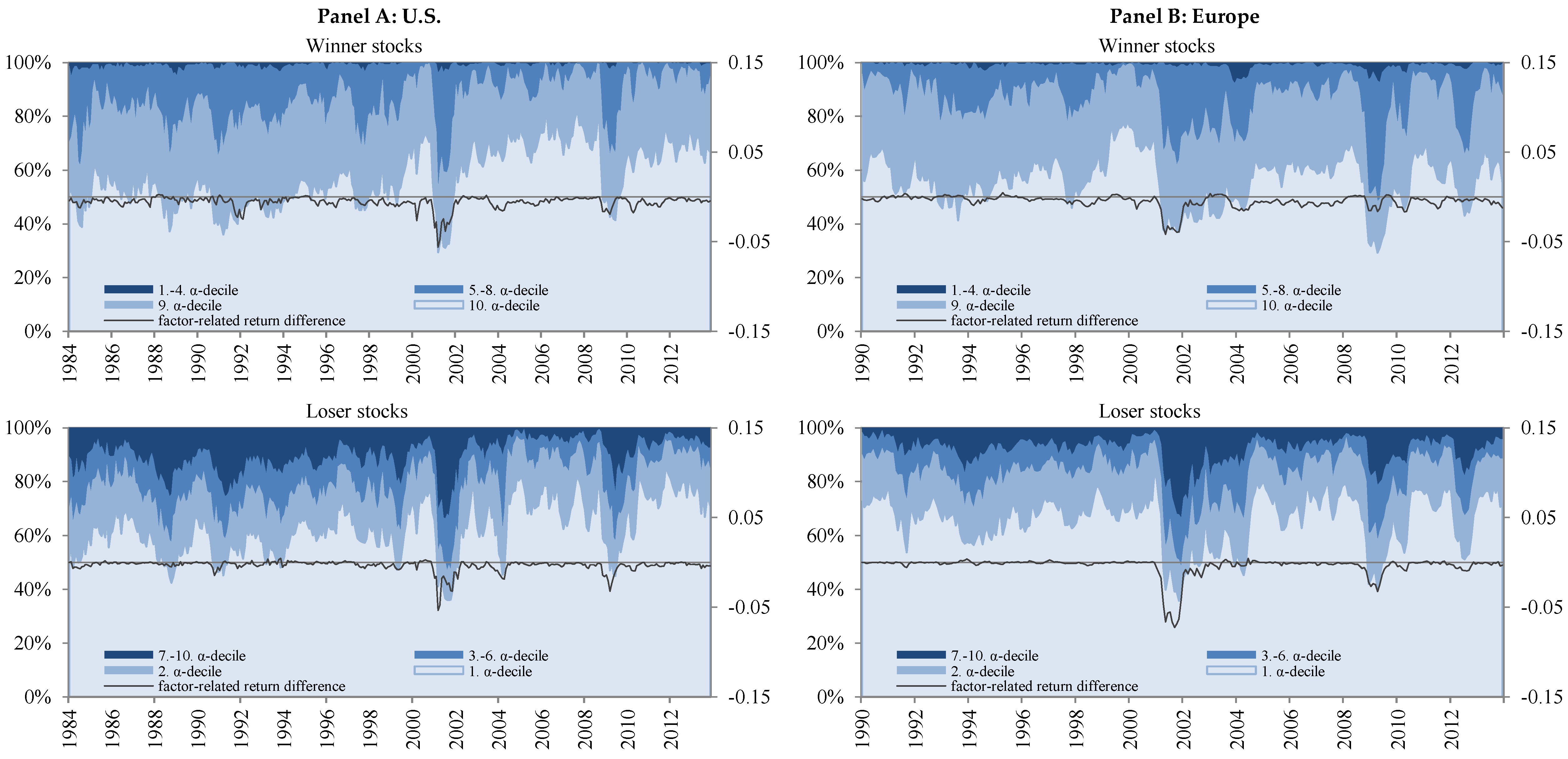
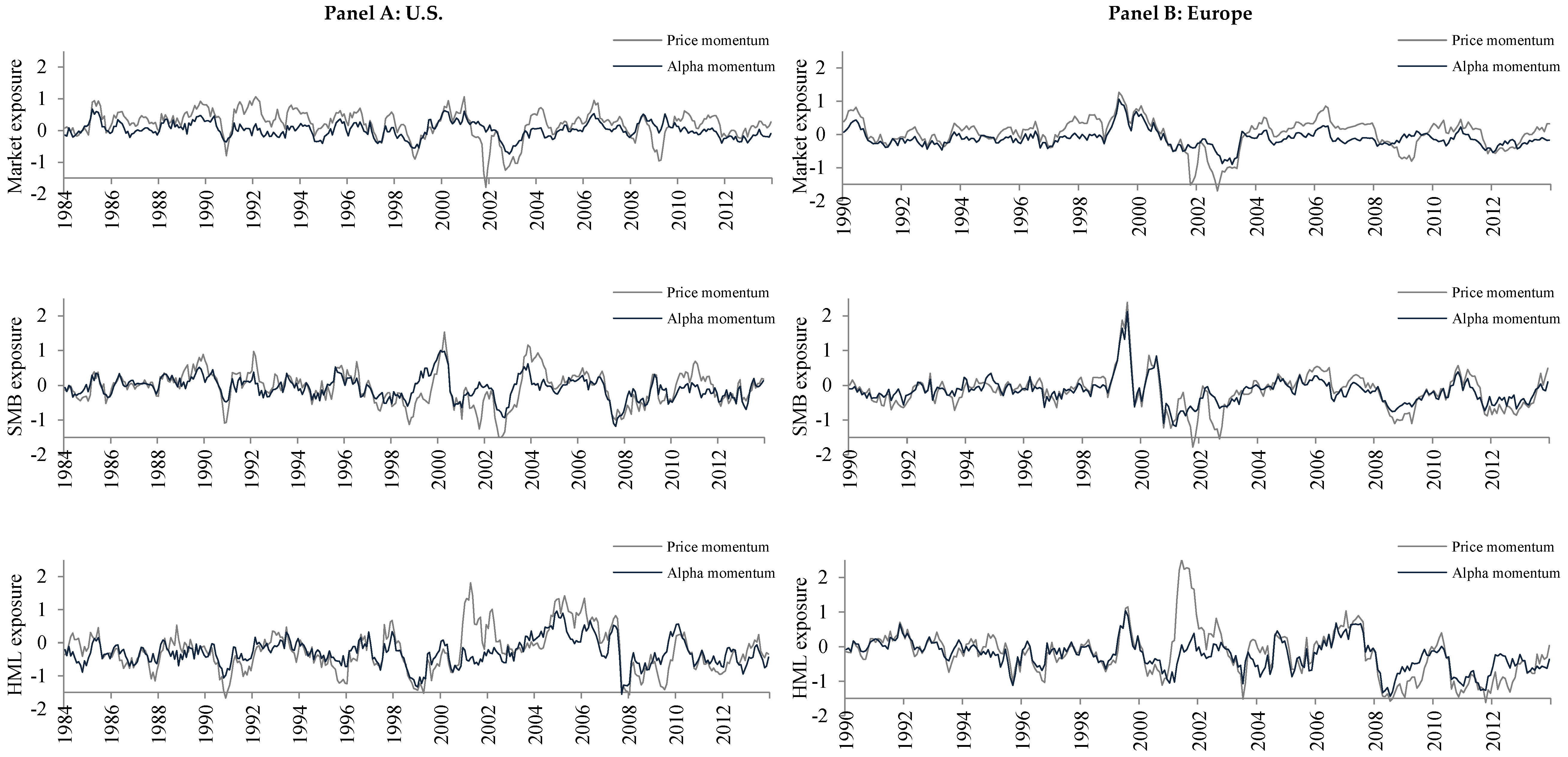
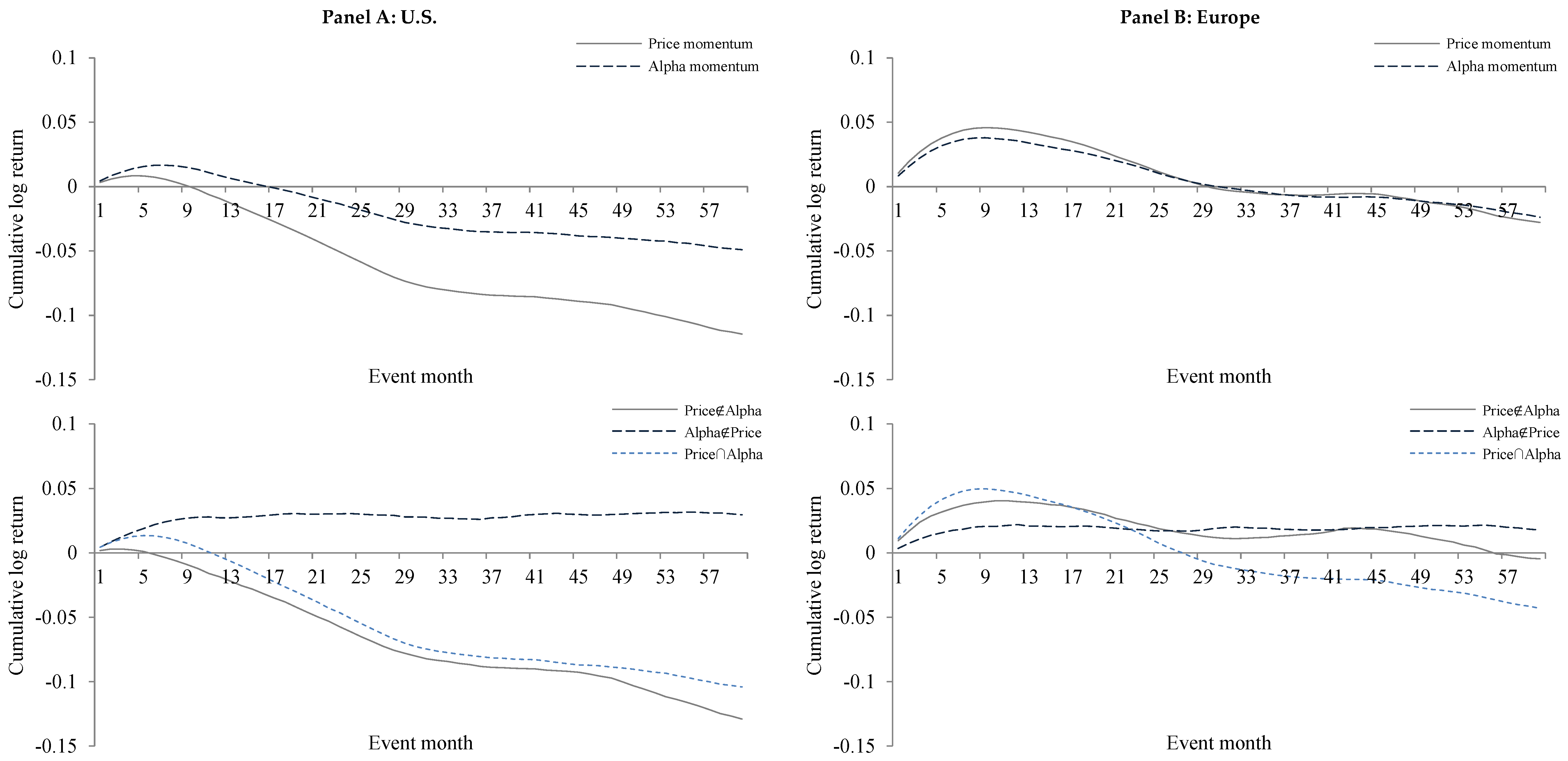
Table 1.
Monthly cross-sectional regressions of individual stock returns based on past return and past alpha.
Table 1.
Monthly cross-sectional regressions of individual stock returns based on past return and past alpha.
| Panel A: U.S. | ||||||
|---|---|---|---|---|---|---|
| Model 1 | Model 2 | Model 3 | ||||
| Mean | t-Value | Mean | t-Value | Mean | t-Value | |
| One-month future return | ||||||
| Intercept | 2.20 | (3.86) | 2.22 | (3.78) | 2.04 | (3.70) |
| log(ME) | −0.14 | (−2.59) | −0.12 | (−2.22) | −0.11 | (−2.05) |
| log(BE/ME) | 0.17 | (1.71) | 0.16 | (1.55) | 0.16 | (1.64) |
| Rt−1 | −3.31 | (−6.24) | −3.15 | (−5.86) | −3.30 | (−6.27) |
| R[t−13,t−2] | 0.23 | (0.83) | −0.21 | (−0.61) | ||
| α[t−13,t−2] | 0.55 | (3.34) | 0.67 | (3.34) | ||
| Six-month future return | ||||||
| Intercept | 15.70 | (2.37) | 15.82 | (2.45) | 14.32 | (2.45) |
| log(ME) | −1.23 | (−1.86) | −1.09 | (−1.89) | −1.02 | (−1.73) |
| log(BE/ME) | 0.94 | (0.98) | 0.97 | (1.00) | 0.89 | (0.99) |
| Rt−1 | −1.51 | (−0.84) | −1.51 | (−0.86) | −1.53 | (−0.87) |
| R[t−13,t−2] | 0.06 | (0.02) | −3.09 | (−1.05) | ||
| α[t−13,t−2] | 1.94 | (1.01) | 4.33 | (2.44) | ||
| Twelve-month future return | ||||||
| Intercept | 31.29 | (2.45) | 31.71 | (2.47) | 28.86 | (2.52) |
| log(ME) | −2.40 | (−1.73) | −2.23 | (−1.64) | −2.03 | (−1.66) |
| log(BE/ME) | 1.23 | (0.66) | 1.24 | (0.68) | 1.16 | (0.68) |
| Rt−1 | 2.75 | (0.82) | 3.09 | (0.93) | 2.64 | (0.80) |
| R[t−13,t−2] | −1.75 | (−0.32) | −6.39 | (−1.17) | ||
| α[t−13,t−2] | 0.90 | (0.25) | 6.16 | (1.65) | ||
| Panel B: Europe | ||||||
| Model 1 | Model 2 | Model 3 | ||||
| Mean | t-Value | Mean | t-Value | Mean | t-Value | |
| One-month future return | ||||||
| Intercept | 0.61 | (1.34) | 0.51 | (1.01) | 0.67 | (1.50) |
| log(ME) | 0.02 | (0.69) | 0.08 | (2.17) | 0.02 | (0.67) |
| log(BE/ME) | 0.33 | (3.58) | 0.36 | (3.43) | 0.32 | (3.59) |
| Rt−1 | −0.58 | (−0.82) | −0.24 | (−0.34) | −0.71 | (−1.05) |
| R[t−13,t−2] | 1.42 | (3.63) | 1.51 | (3.21) | ||
| α[t−13,t−2] | 1.13 | (6.29) | 0.05 | (0.30) | ||
| Six-month future return | ||||||
| Intercept | 9.81 | (1.05) | 10.13 | (1.05) | 9.79 | (1.10) |
| log(ME) | −0.63 | (−0.91) | −0.47 | (−0.67) | −0.57 | (−0.87) |
| log(BE/ME) | 1.96 | (1.29) | 1.99 | (1.33) | 1.90 | (1.32) |
| Rt−1 | 12.36 | (3.49) | 12.09 | (3.63) | 11.82 | (3.45) |
| R[t−13,t−2] | 5.57 | (1.25) | 3.31 | (0.77) | ||
| α[t−13,t−2] | 6.81 | (2.36) | 3.73 | (1.66) | ||
| Twelve-month future return | ||||||
| Intercept | 22.70 | (1.24) | 22.42 | (1.27) | 21.76 | (1.25) |
| log(ME) | −1.57 | (−0.72) | −1.28 | (−0.63) | −1.40 | (−0.67) |
| log(BE/ME) | 3.84 | (1.77) | 3.86 | (1.75) | 3.80 | (1.85) |
| Rt−1 | 24.96 | (4.55) | 24.99 | (4.72) | 24.58 | (4.75) |
| R[t−13,t−2] | 6.06 | (0.82) | 3.22 | (0.61) | ||
| α[t−13,t−2] | 6.56 | (2.92) | 3.90 | (1.68) | ||
Note: This table presents results of monthly cross-sectional regressions of the following form: . The dependent variable is the future return of stock i in month t, its six-month return from t to t + 5, or its twelve-month return from t to t + 11. Independent variables are the market value ( in month t, the book-to-market equity () in month t, past return over month t − 1 (), past return over t − 13 to t − 2 () and past alpha over t − 13 to t − 2 () of stock i. The mean (in %) of the monthly time series of each coefficient is reported in Panel A for the U.S. from January 1984 to December 2013 and in Panel B for Europe from January 1990 to December 2013. We use Newey and West (1987) corrected standard errors to get t-statistics that are robust to heteroskedasticity and autocorrelation.
Table 2.
Monthly performance of different momentum strategies.
| Panel A: U.S. | ||||||||||
|---|---|---|---|---|---|---|---|---|---|---|
| Price Momentum | Alpha Momentum | |||||||||
| µ | SR | α | µadj | µ | SR | α | µadj | |||
| Full evaluation period 01/1984–12/2013 | ||||||||||
| Mean | J12/K1 | 0.75 | 0.11 | 1.08 | 0.60 | 1.04 | 0.24 | 1.24 | 0.96 | |
| t-Value | (2.04) | (3.38) | (2.07) | (3.97) | (4.69) | (4.80) | ||||
| J12/K6 | 0.26 | 0.05 | 0.55 | 0.24 | 0.63 | 0.16 | 0.82 | 0.62 | ||
| (0.74) | (1.92) | (0.85) | (2.45) | (3.41) | (2.97) | |||||
| Sub-period 01/1984–12/1993 | ||||||||||
| J12/K1 | 1.98 | 0.47 | 1.94 | 1.87 | 1.63 | 0.60 | 1.61 | 1.55 | ||
| (5.09) | (6.10) | (4.44) | (6.27) | (6.65) | (5.68) | |||||
| J12/K6 | 1.41 | 0.35 | 1.49 | 1.32 | 1.26 | 0.53 | 1.31 | 1.23 | ||
| (3.94) | (5.33) | (3.59) | (4.95) | (5.85) | (4.66) | |||||
| Sub-period 01/1994–12/2003 | ||||||||||
| J12/K1 | 0.67 | 0.08 | 1.17 | 0.43 | 1.31 | 0.22 | 1.72 | 1.19 | ||
| (0.93) | (1.69) | (0.88) | (2.21) | (3.73) | (3.42) | |||||
| J12/K6 | 0.00 | 0.00 | 0.52 | 0.03 | 0.67 | 0.13 | 1.05 | 0.71 | ||
| (0.00) | (1.10) | (0.09) | (1.17) | (2.72) | (2.29) | |||||
| Sub-period 01/2004–12/2013 | ||||||||||
| J12/K1 | −0.40 | −0,06 | −0.12 | −0.49 | 0.18 | 0.05 | 0.33 | 0.13 | ||
| (−0.51) | (−0.22) | (−0.87) | (0.44) | (0.85) | (0.34) | |||||
| J12/K6 | −0.65 | −0,12 | −0.46 | −0.65 | −0.05 | −0.02 | 0.06 | −0.08 | ||
| (−0.90) | (−0.79) | (−1.16) | (−0.12) | (0.16) | (−0.19) | |||||
| Panel B: Europe | ||||||||||
| Price Momentum | Alpha Momentum | |||||||||
| µ | SR | α | µadj | µ | SR | α | µadj | |||
| Full evaluation period 01/1990–12/2013 | ||||||||||
| Mean | J12/K1 | 2.44 | 0.42 | 2.65 | 2.16 | 1.91 | 0.44 | 2.17 | 1.93 | |
| t-Value | (5.08) | (6.60) | (6.78) | (5.30) | (6.78) | (7.06) | ||||
| J12/K6 | 1.63 | 0.30 | 1.85 | 1.58 | 1.37 | 0.35 | 1.62 | 1.47 | ||
| (3.64) | (4.88) | (5.41) | (4.18) | (5.38) | (5.81) | |||||
| Sub-period 01/1994–12/2003 | ||||||||||
| J12/K1 | 2.90 | 0.41 | 3.13 | 2.46 | 2.01 | 0.36 | 2.49 | 2.19 | ||
| (3.34) | (3.81) | (4.11) | (2.68) | (3.60) | (4.00) | |||||
| J12/K6 | 1.83 | 0.27 | 2.04 | 1.76 | 1.25 | 0.24 | 1.64 | 1.60 | ||
| (2.19) | (2.58) | (3.18) | (1.84) | (2.47) | (3.30) | |||||
| Sub-period 01/2004–12/2013 | ||||||||||
| J12/K1 | 2.21 | 0.46 | 2.57 | 1.92 | 1.95 | 0.66 | 2.15 | 1.80 | ||
| (3.40) | (6.05) | (5.81) | (5.67) | (8.15) | (6.86) | |||||
| J12/K6 | 1.41 | 0.32 | 1.73 | 1.28 | 1.45 | 0.56 | 1.65 | 1.28 | ||
| (2.41) | (4.54) | (4.37) | (4.78) | (6.90) | (4.73) | |||||
Note: This table presents the monthly performance of momentum strategies based on past return and past alpha for a twelve-month formation period (J12) and a one-month (six-month) investment period (K1, K6). For each month t, all stocks with returns for the formation period t − 13 to t − 2 are ranked according to two different criteria. The price momentum strategy indicates winner and loser stocks based on their past return. The alpha momentum strategy ranks stocks based on their past alpha. All momentum strategies are long in an equal-weighted winner portfolio and short in an equal-weighted loser portfolio. For the U.S., Panel A shows the performance of the strategies for the full evaluation period from January 1984 to December 2013 and for three ten-year sub-periods. For Europe, Panel B contains results of the strategies for the full evaluation period from January 1990 to December 2013 and for two ten-year sub-periods. The mean monthly returns (µ), FF alphas (α) and the mean risk-adjusted returns (µadj) are given in %. We use Newey and West (1987) corrected standard errors to get t-statistics that are robust to heteroskedasticity and autocorrelation.
Table 3.
Monthly risk-adjusted returns of two-way dependent sorts on past return and past alpha.
| Panel A: U.S. | ||||||||||
|---|---|---|---|---|---|---|---|---|---|---|
| Portfolios Classified by Past Return | Portfolios Classified by Past Alpha | Alpha Momentum | Portfolios Classified by Past Alpha | Portfolios Classified by Past Return | Price Momentum | |||||
| A5 | A1 | A5–A1 | P5 | P1 | P5–P1 | |||||
| Mean | J12/K1 | P1 | 0.62 | 0.31 | 0.31 | J12/K1 | A1 | 0.18 | 0.26 | −0.08 |
| t-Value | (2.51) | (1.05) | (1.70) | (1.64) | (0.80) | (−0.29) | ||||
| P2 | 0.64 | 0.09 | 0.56 | A2 | 0.18 | 0.35 | −0.17 | |||
| (4.07) | (0.67) | (4.01) | (2.60) | (1.99) | (−1.02) | |||||
| P3 | 0.78 | 0.26 | 0.52 | A3 | 0.33 | 0.39 | −0.06 | |||
| (6.27) | (3.33) | (4.24) | (5.95) | (2.82) | (−0.37) | |||||
| P4 | 1.01 | 0.25 | 0.77 | A4 | 0.45 | 0.69 | −0.25 | |||
| (7.90) | (3.30) | (6.06) | (5.04) | (4.65) | (−1.33) | |||||
| P5 | 1.24 | 0.39 | 0.85 | A5 | 0.89 | 0.93 | −0.04 | |||
| (6.58) | (4.60) | (4.82) | (5.62) | (4.11) | (−0.15) | |||||
| Mean | J12/K6 | P1 | 0.77 | 0.36 | 0.42 | J12/K6 | A1 | 0.31 | 0.41 | −0.10 |
| t-Value | (3.21) | (1.20) | (2.30) | (2.87) | (1.24) | (−0.37) | ||||
| P2 | 0.67 | 0.24 | 0.43 | A2 | 0.23 | 0.40 | −0.17 | |||
| (4.64) | (2.03) | (3.51) | (3.59) | (2.42) | (−1.10) | |||||
| P3 | 0.76 | 0.28 | 0.48 | A3 | 0.33 | 0.51 | −0.17 | |||
| (6.52) | (3.73) | (4.39) | (5.70) | (3.85) | (−1.29) | |||||
| P4 | 0.93 | 0.28 | 0.65 | A4 | 0.41 | 0.69 | −0.28 | |||
| (7.71) | (4.36) | (5.46) | (5.11) | (4.59) | (−1.72) | |||||
| P5 | 0.90 | 0.34 | 0.56 | A5 | 0.67 | 0.95 | −0.28 | |||
| (4.73) | (4.07) | (3.51) | (3.83) | (4.29) | (−1.20) | |||||
| Panel B: Europe | ||||||||||
| Portfolios Classified by Past Return | Portfolios Classified by Past Alpha | Alpha Momentum | Portfolios Classified by Past Alpha | Portfolios Classified by Past Return | Price Momentum | |||||
| A5 | A1 | A5–A1 | P5 | P1 | P5–P1 | |||||
| Mean | J12/K1 | P1 | −0.70 | −1.18 | 0.47 | J12/K1 | A1 | −0.18 | −1.29 | 1.11 |
| t-Value | (−2.50) | (−3.24) | (1.73) | (−0.95) | (−3.26) | (3.49) | ||||
| P2 | −0.06 | −0.34 | 0.28 | A2 | 0.09 | −0.69 | 0.78 | |||
| (−0.26) | (−1.71) | (1.55) | (0.63) | (−2.95) | (3.57) | |||||
| P3 | 0.27 | −0.07 | 0.34 | A3 | 0.32 | −0.26 | 0.59 | |||
| (1.48) | (−0.47) | (2.33) | (2.56) | (−1.43) | (2.78) | |||||
| P4 | 0.53 | 0.19 | 0.35 | A4 | 0.62 | −0.04 | 0.65 | |||
| (2.85) | (1.46) | (2.07) | (3.93) | (−0.19) | (2.89) | |||||
| P5 | 1.61 | 0.52 | 1.09 | A5 | 1.55 | 0.10 | 1.46 | |||
| (3.72) | (3.15) | (2.57) | (3.40) | (0.34) | (3.02) | |||||
| Mean | J12/K6 | P1 | −0.35 | −0.98 | 0.62 | J12/K6 | A1 | −0.08 | −1.05 | 0.97 |
| t-Value | (−1.28) | (−2.93) | (2.88) | (−0.43) | (−3.00) | (3.49) | ||||
| P2 | −0.01 | −0.22 | 0.21 | A2 | 0.11 | −0.44 | 0.54 | |||
| (−0.03) | (−1.17) | (1.29) | (0.86) | (−1.98) | (2.63) | |||||
| P3 | 0.23 | 0.02 | 0.22 | A3 | 0.28 | −0.15 | 0.43 | |||
| (1.25) | (0.11) | (1.38) | (2.44) | (−0.79) | (2.15) | |||||
| P4 | 0.48 | 0.20 | 0.27 | A4 | 0.51 | 0.00 | 0.51 | |||
| (2.48) | (1.65) | (1.70) | (4.02) | (−0.02) | (2.36) | |||||
| P5 | 0.93 | 0.42 | 0.51 | A5 | 0.89 | 0.19 | 0.70 | |||
| (2.28) | (3.14) | (1.34) | (2.10) | (0.66) | (1.55) | |||||
Note: This table presents the mean risk-adjusted returns of two-way dependent sorts on past return and past alpha for a twelve-month formation period (J12) and a one-month (six-month) investment period (K1, K6). For each month t, all stocks with returns for the formation period t − 13 to t − 2 are first sorted into quintiles according to past return (past alpha), then further ranked by past alpha (past return) within each quintile. The table contains results for equal-weighted winner (P5, A5), loser (P1, A1) and zero-investment portfolios (P5–P1, A5–A1). For the U.S., Panel A shows the risk-adjusted return (%) of the strategies for the full evaluation period from January 1984 to December 2013. For Europe, Panel B contains results of the strategies for the full evaluation period from January 1990 to December 2013. We use Newey and West (1987) corrected standard errors to get t-statistics that are robust to heteroskedasticity and autocorrelation.
Table 4.
Monthly risk-adjusted returns of double-sorting stocks on the same criterion.
| Panel A: U.S. | ||||||||||
|---|---|---|---|---|---|---|---|---|---|---|
| Portfolios Classified by Past Return | Portfolios Classified by Past Return | Price Momentum | Portfolios Classified by Past Alpha | Portfolios Classified by Past Alpha | Alpha Momentum | |||||
| P5 | P1 | P5–P1 | A5 | A1 | A5–A1 | |||||
| Mean | J12/K1 | P1 | 0.38 | 0.39 | −0.01 | J12/K1 | A1 | 0.26 | 0.33 | −0.08 |
| t-Value | (2.68) | (1.12) | (−0.04) | (2.12) | (1.17) | (−0.36) | ||||
| P2 | 0.36 | 0.24 | 0.12 | A2 | 0.30 | 0.26 | 0.05 | |||
| (4.89) | (2.09) | (1.49) | (4.23) | (2.35) | (0.61) | |||||
| P3 | 0.49 | 0.45 | 0.04 | A3 | 0.46 | 0.30 | 0.16 | |||
| (7.24) | (6.35) | (0.60) | (7.38) | (4.40) | (2.42) | |||||
| P4 | 0.63 | 0.49 | 0.14 | A4 | 0.69 | 0.52 | 0.17 | |||
| (8.68) | (8.10) | (1.89) | (7.58) | (8.10) | (2.21) | |||||
| P5 | 0.86 | 0.67 | 0.19 | A5 | 1.23 | 0.75 | 0.48 | |||
| (5.47) | (7.26) | (1.27) | (6.03) | (7.96) | (2.78) | |||||
| Mean | J12/K6 | P1 | 0.42 | 0.50 | −0.07 | J12/K6 | A1 | 0.32 | 0.38 | −0.06 |
| t-Value | (3.02) | (1.42) | (−0.30) | (2.72) | (1.32) | (−0.31) | ||||
| P2 | 0.38 | 0.34 | 0.04 | A2 | 0.32 | 0.30 | 0.02 | |||
| (5.26) | (2.87) | (0.60) | (4.82) | (2.92) | (0.44) | |||||
| P3 | 0.45 | 0.43 | 0.01 | A3 | 0.43 | 0.36 | 0.07 | |||
| (7.93) | (6.40) | (0.37) | (7.65) | (5.88) | (2.03) | |||||
| P4 | 0.54 | 0.50 | 0.05 | A4 | 0.63 | 0.47 | 0.16 | |||
| (8.30) | (8.87) | (1.13) | (7.80) | (8.00) | (3.46) | |||||
| P5 | 0.65 | 0.58 | 0.07 | A5 | 1.02 | 0.70 | 0.32 | |||
| (3.74) | (8.16) | (0.52) | (4.87) | (7.83) | (2.01) | |||||
| Panel B: Europe | ||||||||||
| Portfolios Classified by Past Return | Portfolios Classified by Past Return | Price Momentum | Portfolios Classified by Past Alpha | Portfolios Classified by Past Alpha | Alpha Momentum | |||||
| P5 | P1 | P5–P1 | A5 | A1 | A5–A1 | |||||
| Mean | J12/K1 | P1 | −0.42 | −1.19 | 0.77 | J12/K1 | A1 | −0.33 | −1.06 | 0.73 |
| t-Value | (−2.98) | (−3.78) | (2.98) | (−2.65) | (−3.99) | (3.40) | ||||
| P2 | −0.04 | −0.32 | 0.29 | A2 | −0.07 | −0.30 | 0.23 | |||
| (−0.41) | (−2.66) | (3.11) | (−1.01) | (−2.73) | (2.58) | |||||
| P3 | 0.19 | 0.05 | 0.15 | A3 | 0.24 | −0.05 | 0.29 | |||
| (2.14) | (0.44) | (1.85) | (3.05) | (−0.64) | (4.39) | |||||
| P4 | 0.49 | 0.24 | 0.25 | A4 | 0.43 | 0.23 | 0.20 | |||
| (4.98) | (2.79) | (3.31) | (4.19) | (2.81) | (2.40) | |||||
| P5 | 1.57 | 0.55 | 1.01 | A5 | 1.37 | 0.53 | 0.84 | |||
| (4.15) | (5.34) | (2.91) | (3.80) | (4.93) | (2.81) | |||||
| Mean | J12/K6 | P1 | −0.33 | −0.92 | 0.59 | J12/K6 | A1 | −0.26 | −0.86 | 0.61 |
| t-Value | (−2.73) | (−3.35) | (2.81) | (−2.64) | (−3.62) | (3.43) | ||||
| P2 | 0.03 | −0.22 | 0.25 | A2 | 0.01 | −0.17 | 0.18 | |||
| (0.39) | (−2.06) | (4.25) | (0.14) | (−2.08) | (3.99) | |||||
| P3 | 0.20 | 0.04 | 0.16 | A3 | 0.23 | 0.02 | 0.21 | |||
| (2.92) | (0.49) | (3.80) | (3.30) | (0.25) | (5.67) | |||||
| P4 | 0.40 | 0.22 | 0.18 | A4 | 0.39 | 0.22 | 0.17 | |||
| (4.71) | (2.92) | (3.97) | (4.57) | (3.14) | (3.29) | |||||
| P5 | 1.01 | 0.46 | 0.56 | A5 | 0.94 | 0.47 | 0.47 | |||
| (2.97) | (4.77) | (1.75) | (2.76) | (4.89) | (1.67) | |||||
Note: This table presents the mean risk-adjusted returns of double-sorting stocks on the same criterion for a twelve-month formation period (J12) and a one-month (six-month) investment period (K1, K6). For each month t, all stocks with returns for the formation period t − 13 to t − 2 are first sorted into quintiles according to past return (past alpha), then further ranked by past return (past alpha) within each quintile. The table contains results for equal-weighted winner (P5, A5), loser (P1, A1) and zero-investment portfolios (P5–P1, A5–A1). For the U.S., Panel A shows the risk-adjusted return (%) of the strategies for the full evaluation period from January 1984 to December 2013. For Europe, Panel B contains results of the strategies for the full evaluation period from January 1990 to December 2013. We use Newey and West (1987) corrected standard errors to get t-statistics that are robust to heteroskedasticity and autocorrelation.
Table 5.
Dominance of momentum strategies in the cross-section of individual stock returns.
| Panel B: U.S. | |||
|---|---|---|---|
| Mean | t-Value | ||
| J12/K1 | Intercept | 2.05 | (4.38) |
| Rt−1 | −0.10 | (−2.33) | |
| log(ME) | 0.14 | (1.38) | |
| log(BE/ME) | −3.48 | (−6.66) | |
| P10 | 0.20 | (1.22) | |
| P1 | −0.02 | (−0.06) | |
| A10 | 0.54 | (3.21) | |
| A1 | −0.22 | (−1.67) | |
| P10–P1 | 0.22 | (0.61) | |
| A10–A1 | 0.76 | (3.64) | |
| J12/K6 | Intercept | 2.07 | (4.69) |
| Rt−1 | −0.10 | (−2.55) | |
| log(ME) | 0.13 | (1.44) | |
| log(BE/ME) | −3.44 | (−6.96) | |
| P10 | 0.04 | (0.25) | |
| P1 | 0.17 | (0.65) | |
| A10 | 0.35 | (2.39) | |
| P10–P1 | −0.13 | (−0.39) | |
| A10–A1 | 0.61 | (2.91) | |
| Panel B: Europe | |||
| Mean | t-Value | ||
| J12/K1 | Intercept | 0.77 | (1.70) |
| Rt−1 | 0.04 | (0.98) | |
| log(ME) | 0.31 | (3.35) | |
| log(BE/ME) | −0.38 | (−0.55) | |
| P10 | 1.07 | (4.88) | |
| P1 | −0.81 | (−3.00) | |
| A10 | 0.27 | (2.05) | |
| A1 | −0.26 | (−2.08) | |
| P10–P1 | 1.88 | (4.79) | |
| A10–A1 | 0.53 | (2.78) | |
| J12/K6 | Intercept | 0.78 | (1.78) |
| Rt−1 | 0.04 | (1.20) | |
| log(ME) | 0.33 | (3.57) | |
| log(BE/ME) | −0.22 | (−0.30) | |
| P10 | 0.65 | (3.04) | |
| P1 | −0.58 | (−2.36) | |
| A10 | 0.20 | (1.58) | |
| A1 | −0.30 | (−3.00) | |
| P10–P1 | 1.23 | (3.37) | |
| A10–A1 | 0.50 | (2.96) | |
Note: This table presents results of monthly cross-sectional regressions of the following form: . The dependent variable is the one-month future return of stock i in month t. Independent variables are the market capitalization () in month t, the book-to-market-equity () in month t and the past return of the stock () in month t − 1. P10 (P1) is a dummy variable that equals one if stock i’s past return over t − 13 to t − 2 is ranked in the winner (loser) decile. A10 (A1) is a dummy variable that equals one if stock i’s past alpha over t − 13 to t − 2 is ranked in the winner (loser) decile. For the J12/K1 strategy, we implement one cross-sectional regression for the one cohort held in each investment month. The J12/K6 strategy consists of six overlapping cohorts each month. Thus, we run one cross-sectional regression for each of the six cohorts held in month t. The mean (in %) of the monthly time series of each coefficient is reported in Panel A for the U.S. from January 1984 to December 2013 and in Panel B for Europe from January 1990 to December 2013. We use Newey and West (1987) corrected standard errors to get t-statistics that are robust to heteroskedasticity and autocorrelation.
Table 6.
Monthly performance of different subset strategies.
| Panel A: U.S. | |||||||||||||
|---|---|---|---|---|---|---|---|---|---|---|---|---|---|
| Price ∉ Alpha | Price ∩ Alpha | Alpha ∉ Price | |||||||||||
| µ | SR | α | µadj | µ | SR | α | µadj | µ | SR | α | µadj | ||
| Full evaluation period 01/1984–12/2013 | |||||||||||||
| Mean | J12/K1 | 0.40 | 0.05 | 0.74 | 0.15 | 1.03 | 0.16 | 1.33 | 0.90 | 1.04 | 0.25 | 1.16 | 1.09 |
| t-Value | (1.00) | (2.22) | (0.47) | (2.78) | (3.91) | (2.98) | (4.10) | (4.41) | (5.82) | ||||
| J12/K6 | −0.07 | −0.01 | 0.24 | −0.14 | 0.49 | 0.09 | 0.77 | 0.47 | 0.84 | 0.23 | 0.97 | 0.85 | |
| (−0.20) | (0.86) | (−0.49) | (1.38) | (2.43) | (1.60) | (3.42) | (4.08) | (4.50) | |||||
| Sub-period 01/1984–12/1993 | |||||||||||||
| J12/K1 | 1.53 | 0.31 | 1.47 | 1.46 | 2.40 | 0.57 | 2.38 | 2.25 | 0.75 | 0.30 | 0.75 | 0.64 | |
| (4.38) | (4.81) | (3.50) | (6.28) | (6.45) | (5.53) | (3.28) | (3.31) | (2.77) | |||||
| J12/K6 | 1.13 | 0.24 | 1.19 | 0.99 | 1.66 | 0.42 | 1.77 | 1.62 | 0.74 | 0.38 | 0.74 | 0.67 | |
| (3.04) | (3.58) | (2.41) | (4.45) | (6.14) | (4.26) | (3.44) | (3.35) | (2.79) | |||||
| Sub-period 01/1994–12/2003 | |||||||||||||
| J12/K1 | 0.15 | 0.01 | 0.52 | −0.18 | 0.97 | 0.12 | 1.54 | 0.78 | 1.68 | 0.30 | 1.95 | 1.73 | |
| (0.20) | (0.69) | (−0.31) | (1.28) | (2.35) | (1.54) | (2.58) | (4.16) | (4.63) | |||||
| J12/K6 | −0.58 | −0.07 | −0.11 | −0.43 | 0.37 | 0.05 | 0.89 | 0.35 | 1.19 | 0.22 | 1.44 | 1.18 | |
| (−0.94) | (−0.21) | (−0.98) | (0.56) | (1.89) | (0.87) | (1.80) | (3.11) | (3.07) | |||||
| Sub-period 01/2004–12/2013 | |||||||||||||
| J12/K1 | −0.50 | −0.06 | −0.16 | −0.83 | −0.27 | −0.05 | −0.06 | −0.35 | 0.70 | 0.19 | 0.81 | 0.89 | |
| (−0.55) | (−0.24) | (−1.38) | (−0.40) | (−0.11) | (−0.63) | (2.10) | (2.17) | (2.74) | |||||
| J12/K6 | −0.77 | −0.12 | −0.53 | −1.00 | −0.55 | −0.11 | −0.41 | −0.55 | 0.60 | 0.21 | 0.70 | 0.70 | |
| (−0.99) | (−0.88) | (−1.73) | (−0.81) | (−0.69) | (−0.91) | (2.47) | (2.96) | (2.19) | |||||
| Panel B: Europe | |||||||||||||
| Price ∉ Alpha | Price ∩ Alpha | Alpha ∉ Price | |||||||||||
| µ | SR | α | µadj | µ | SR | α | µadj | µ | SR | α | µadj | ||
| Full evaluation period 01/1990–12/2013 | |||||||||||||
| Mean | J12/K1 | 2.17 | 0.35 | 2.23 | 1.74 | 2.58 | 0.43 | 2.86 | 2.43 | 0.78 | 0.25 | 0.99 | 0.96 |
| t-Value | (4.89) | (6.34) | (5.72) | (5.25) | (6.59) | (7.09) | (3.48) | (5.51) | (5.28) | ||||
| J12/K6 | 1.37 | 0.27 | 1.50 | 1.21 | 1.79 | 0.33 | 2.05 | 1.83 | 0.70 | 0.27 | 0.90 | 0.84 | |
| (3.28) | (4.87) | (4.47) | (3.87) | (4.92) | (5.69) | (3.69) | (6.10) | (5.10) | |||||
| Sub-period 01/1994–12/2003 | |||||||||||||
| J12/K1 | 2.51 | 0.32 | 2.30 | 1.65 | 3.01 | 0.39 | 3.44 | 2.88 | 0.56 | 0.14 | 0.99 | 0.85 | |
| (3.45) | (3.76) | (4.45) | (3.08) | (3.69) | (4.27) | (1.16) | (3.11) | (2.39) | |||||
| J12/K6 | 1.53 | 0.23 | 1.50 | 0.97 | 1.95 | 0.28 | 2.29 | 2.13 | 0.42 | 0.13 | 0.81 | 0.75 | |
| (2.12) | (2.66) | (3.15) | (2.14) | (2.55) | (3.45) | (1.06) | (3.44) | (2.64) | |||||
| Sub-period 01/2004–12/2013 | |||||||||||||
| J12/K1 | 2.04 | 0.37 | 1.87 | 1.65 | 2.40 | 0.54 | 2.42 | 2.11 | 0.95 | 0.41 | 1.06 | 1.13 | |
| (2.79) | (2.35) | (4.45) | (4.32) | (3.89) | (6.26) | (4.48) | (4.96) | (5.10) | |||||
| J12/K6 | 1.11 | 0.23 | 0.97 | 0.97 | 1.63 | 0.41 | 1.61 | 1.45 | 0.85 | 0.44 | 0.99 | 0.87 | |
| (1.76) | (1.31) | (3.15) | (3.07) | (2.82) | (4.48) | (4.60) | (5.35) | (3.55) | |||||
Note: This table presents the monthly performance of momentum strategies based on past return and past alpha for a twelve-month formation period (J12) and a one-month (six-month) investment period (K1, K6). For each month t, all stocks with returns for the formation period t − 13 to t − 2 are ranked according to three different criteria. The “Price ∉ Alpha” momentum strategy buys (sells) stocks that are in the winner (loser) decile based on past return, but not based on past alpha. The “Price ∩ Alpha” momentum strategy invests in those stocks that can be in the two extreme deciles according to both past return and past alpha at the same time. The “Alpha ∉ Price” momentum strategy contains stocks that are winner or loser stocks based on their past alpha, but not on their past return. All momentum strategies are long in an equal-weighted winner portfolio and short in an equal-weighted loser portfolio. For the U.S., Panel A shows the performance of the strategies for the full evaluation period from January 1984 to December 2013 and for three ten-year sub-periods. For Europe, Panel B contains results of the strategies for the full evaluation period from January 1990 to December 2013 and for two ten-year sub-periods. The mean monthly returns (µ), FF alphas (α) and the mean risk-adjusted returns (µadj) are given in %. We use Newey and West (1987) corrected standard errors to get t-statistics that are robust to heteroskedasticity and autocorrelation.
Table 7.
Monthly risk-adjusted returns of momentum strategies and sentiment.
| Panel A: U.S. | ||||||||
|---|---|---|---|---|---|---|---|---|
| Price Momentum | Alpha Momentum | |||||||
| P10 | P1 | P10–P1 | A10 | A1 | A10–A1 | |||
| Mean | J12/K1 | Optimistic | 1.09 | −0.20 | 1.29 | 1.13 | −0.10 | 1.23 |
| t-Value | (5.63) | (−0.58) | (3.40) | (4.41) | (−0.34) | (4.51) | ||
| Pessimistic | 0.82 | 0.97 | −0.15 | 1.24 | 0.61 | 0.63 | ||
| (5.36) | (2.08) | (−0.30) | (6.78) | (1.62) | (1.82) | |||
| Opt.-Pes. | 0.27 | −1.17 | 1.44 | −0.11 | −0.71 | 0.60 | ||
| (1.22) | (−2.00) | (2.28) | (−0.38) | (−1.48) | (1.36) | |||
| Mean | J12/K6 | Optimistic | 0.85 | 0.00 | 0.85 | 0.86 | 0.04 | 0.82 |
| t-Value | (4.32) | (0.00) | (2.54) | (3.48) | (0.15) | (3.36) | ||
| Pessimistic | 0.60 | 1.03 | −0.43 | 1.10 | 0.72 | 0.38 | ||
| (4.42) | (2.52) | (−0.98) | (6.40) | (2.04) | (1.18) | |||
| Opt.-Pes. | 0.25 | −1.04 | 1.29 | −0.23 | −0.67 | 0.44 | ||
| (1.15) | (−1.96) | (2.31) | (−0.82) | (−1.50) | (1.10) | |||
| Panel B: Europe | ||||||||
| Price Momentum | Alpha Momentum | |||||||
| P10 | P1 | P10–P1 | A10 | A1 | A10–A1 | |||
| Mean | J12/K1 | Optimistic | 1.72 | −1.03 | 2.75 | 1.55 | −0.93 | 2.48 |
| t-Value | (3.95) | (−3.14) | (5.33) | (3.49) | (−3.50) | (5.55) | ||
| Pessimistic | 0.75 | −0.82 | 1.57 | 0.64 | −0.73 | 1.37 | ||
| (3.99) | (−2.26) | (4.22) | (2.56) | (−2.27) | (4.59) | |||
| Opt.-Pes. | 0.97 | −0.21 | 1.18 | 0.91 | −0.20 | 1.11 | ||
| (2.07) | (−0.41) | (1.79) | (1.80) | (−0.48) | (2.03) | |||
| Mean | J12/K6 | Optimistic | 1.13 | −0.76 | 1.90 | 1.09 | −0.72 | 1.81 |
| t-Value | (2.95) | (−2.35) | (3.95) | (2.78) | (−2.69) | (4.44) | ||
| Pessimistic | 0.58 | −0.68 | 1.26 | 0.51 | −0.62 | 1.13 | ||
| (3.57) | (−2.03) | (3.84) | (2.06) | (−2.07) | (4.14) | |||
| Opt.-Pes. | 0.55 | −0.08 | 0.63 | 0.58 | −0.10 | 0.68 | ||
| (1.34) | (−0.17) | (1.05) | (1.27) | (−0.24) | (1.35) | |||
Note: This table presents the mean risk-adjusted returns of momentum strategies based on past return and past alpha for a twelve-month formation period (J12) and a one-month (six-month) investment period (K1, K6) in different sentiment periods. Following Stambaugh et al. (2012), we define an investment month t as optimistic (pessimistic) if the sentiment index in month t − 1 is above (below) the median. For each month t, all stocks with returns for the formation period t − 13 to t − 2 are ranked according to two different criteria. The price momentum strategy indicates winner and loser stocks based on their past return. The alpha momentum strategy ranks stocks based on their past alpha. The table contains results for equal-weighted winner (P5, A5), loser (P1, A1) and zero-investment portfolios (P5–P1, A5–A1). For the U.S., Panel A shows the risk-adjusted return (%) of the strategies for the full evaluation period from January 1984 to December 2013. For Europe, Panel B contains results of the strategies for the full evaluation period from January 1990 to December 2013. We use Newey and West (1987) corrected standard errors to get t-statistics that are robust to heteroskedasticity and autocorrelation.
© 2018 by the authors. Licensee MDPI, Basel, Switzerland. This article is an open access article distributed under the terms and conditions of the Creative Commons Attribution (CC BY) license (http://creativecommons.org/licenses/by/4.0/).
Share and Cite
MDPI and ACS Style
Hühn, H.L.; Scholz, H. Alpha Momentum and Price Momentum. Int. J. Financial Stud. 2018, 6, 49. https://doi.org/10.3390/ijfs6020049
AMA Style
Hühn HL, Scholz H. Alpha Momentum and Price Momentum. International Journal of Financial Studies. 2018; 6(2):49. https://doi.org/10.3390/ijfs6020049
Chicago/Turabian StyleHühn, Hannah Lea, and Hendrik Scholz. 2018. "Alpha Momentum and Price Momentum" International Journal of Financial Studies 6, no. 2: 49. https://doi.org/10.3390/ijfs6020049
Note that from the first issue of 2016, this journal uses article numbers instead of page numbers. See further details here.