British-European Trade Relations and Brexit: An Empirical Analysis of the Impact of Economic and Financial Uncertainty on Exports

Abstract

Brexit, the withdrawal of the United Kingdom (UK) from the European Union (EU), has led to significant exchange rate fluctuations and to uncertainty in financial markets and in UK–EU trade relations. In this article, we use a non-linear model to study how this uncertainty affects export companies. Exports tend to react in spurts when exchange rate fluctuations go beyond a band of inaction, referred to here as a “play area”. We apply an algorithm to study this hysteretic relationship with ordinary least squares (OLS) regressions. We examine the export relationship between Europe (Belgium, Germany, France, Italy, and The Netherlands) and the UK. To guarantee the robustness of the results, we estimate a variety of specifications for modeling economic uncertainty: (a) constant uncertainty, (b) exchange rate volatility, (c) volatility in European equity markets, (d) the Treasury Bill EuroDollar Difference (TED-spread), (e) the Economic Policy Uncertainty Index (EPUI), and (f) a combination of exchange rate volatility and the EPUI. Since the results show little evidence of hysteretic effects on British exports, we focus on the European side. The specifications including exchange rate and equity market volatility show a significant effect of hysteresis.

1. Introduction

Significant exchange rate fluctuations have a major effect on export companies’ profits and losses. The devaluation of the pound since the Brexit vote is a crucial issue at present for exporting countries in the European Union (EU). Although it was then Prime Minister David Cameron who called the referendum during his premiership, he also warned against the negative impacts of leaving the EU.

“At the core of the European Union must be, as it is now, the single market. Britain is at the heart of that Single Market, and must remain so. […] However, when the Single Market remains in-complete […] it is only half the success it could be. We would need to weigh up very carefully the consequences of no longer being inside the EU and its single market, as a full member.”

(Cameron 2013)

The Brexit process has now formally begun, calling the political relationship between the United Kingdom (UK) and Europe fundamentally into question. It can be expected to affect not only diplomatic relationships and political cooperation between the EU and the UK but also joint trade. It is likely that the UK will lose access to the European Single Market. This, along with uncertainty about future bilateral trade relations, is a concern for numerous companies as well as politicians and policy makers. According to a survey conducted by the Bertelsmann Foundation, 36% of companies headquartered in Germany or the UK expect negative impacts on their business activities (Bertelsmann-Stiftung 2016).

2. Path-Dependency and the European Single Market

Hysteresis describes a model characteristic due to which shocks on the endogenous variable have a long-term, persistent effect. It may occur in various contexts, such as the pricing-to-market strategy of export companies. Since a substantial investment is required to enter the export market, companies may have an interest in keeping their sales prices in foreign currencies stable. To do so, companies will absorb smaller exchange rate fluctuations and only adapt prices to the exchange rate asymmetrically, when certain thresholds are exceeded (Fedoseeva and Werner 2014).

This paper is concerned with hysteresis in international trade relations. The classical theory describes a simple relationship between exchange rates and exports: when a country’s currency depreciates, exports increase, and vice versa (Belke and Polleit 2009, p. 622; Belke and Volz 2015). This is a strictly macroeconomic perspective, and one that fails to consider a number of interactions. This basic relationship remains essentially unchanged if one assumes hysteretic effects on a country’s exports. In this paper, we also include microeconomic effects in addition to macroeconomic relationships in our proposed explanation. The two key points here are sunk costs and uncertainty. In relation to export activity, sunk costs may include the costs of marketing or setting up the logistics or infrastructure for exports (Baldwin and Krugman 1989). As soon as these investments have been made, they play a minor role in further calculations. This is based on the assumption that these kinds of capital investments can no longer, or can only partly be converted into liquidity. After a company’s decision to enter the export market, the only relevant issue is whether the variable unit costs are covered.

On the microeconomic level, this leads into areas where companies do not react to exchange rate changes, which is referred to as a “band of inaction” (Belke et al. 2014). The underlying argumentation is that a company that is not active on the export market initially has to cover market entry costs. These include the expenses of creating the appropriate infrastructure and the costs of marketing. Only if the exchange rate exceeds the level at which not only variable unit costs but also sunk costs are covered will the company enter the export market, or in the reverse case, leave the market. Uncertainty about future economic trends leads to similar arguments and widens the band of inaction,1 since it then makes more sense to wait and see, for instance, how the exchange rate develops. A decision is only made if trends continue over a longer period. The option value of waiting rises with increasing uncertainty (Côté 1994). If the exchange rate is favorable enough for market entry (i.e., if the domestic currency has depreciated against the foreign currency) and a company has therefore entered the export market, this does not mean that a reversal of the exchange rate development will lead to the company immediately exiting the market. In this case, if there are sunk costs, the company will not immediately stop exporting its goods. Instead, it will stay in the export market as long as variable unit costs are covered (Belke et al. 2013). These relationships lead to persistent effects of exchange rate shocks.

Shifting to the macroeconomic perspective, the aggregation of individual companies means—as is the case in the microeconomic perspective—that areas form in which exchange rates have only a minor effect on exports, which are referred to as “play areas” (Belke et al. 2013, 2014). These areas become relevant when the exchange rate shows only minimal fluctuations. Such small exchange rate fluctuations only cross the threshold for entering or leaving the export sector for a few companies. If the exchange rate moves in one direction far enough and for a long enough period of time, exports show an even stronger spurt reaction to exchange rate fluctuations (Belke et al. 2013), since for many companies, the critical level has been reached.

With regard to trade relations between Europe and the United Kingdom, one can assume that hysteretic effects exist. This is particularly likely since the United Kingdom is a member of the European Union but not the Monetary Union. This means that exchange rate fluctuations will continue to play a role in trade with the United Kingdom into the future.2 At the same time, the United Kingdom is still part of the Single Market, at least for the foreseeable future. For trade with other member states, this means significantly decreased sunk costs through the dismantling of trade barriers such as tariffs. With the UK’s upcoming Brexit, however, it is still unclear what position Europe will adopt toward the United Kingdom. Leaving the EU will probably mean that the United Kingdom loses its member status in the European Single Market. It is difficult to predict whether it will be possible for the British government to negotiate a special status for the United Kingdom, and if so, what this would look like specifically. If the United Kingdom loses its trade privileges completely, one has to assume that hysteresis will have a more significant effect on trade flows than it has up to now, since the increased costs will widen the band of inaction.

A further example of the significance of hysteresis in European trade with the United Kingdom is the low exchange rate elasticity of German exports in the important machinery and transport equipment sector. Belke et al. (2013) attribute this in part to the high market power German companies in these sectors have. As a result, exchange rate fluctuations will have much stronger long-term effects in this area than are evident at the present point in time.

3. Brief Literature Review

Baldwin and Krugman (1989), as well as Dixit (1989), laid the foundations for empirical studies of hysteresis in exports.

This article is based on a series of recent empirical studies that have used an algorithm to determine the concrete size of the play area. The first of these was a 2014 paper providing an overview of various possibilities for empirical modeling of hysteretic effects (Belke et al. 2014). In the same year, Belke et al. (2013) introduced an approach that has also been adopted in this paper to test the existence of hysteresis in German export relationships. Their study, which was limited to a constant play area, concluded that hysteresis is relevant for the majority of German exports. In another paper, the same methodology was applied to Greek imports, but this time with a variable play component based on the economic policy uncertainty index (EPUI) (Belke and Kronen 2015). Also in 2015, Belke et al. (2015a) published an article studying Eurozone exports to the United States, also assuming a variable play area. Here, instead of the EPUI, they used the volatility of the real exchange rate as the basis for the variable play component.

In a further paper, Belke et al. (2015b) also assumed hysteresis in export dynamics. Here, instead of determining the play area based on the development of the exchange rate, they used companies’ capacity utilization rates. They argued that the rate of capacity utilization has an influence on the relationship between domestic demand and companies’ export market activities. Based on these considerations, they applied a smooth transition regression model to study the existence of a nonlinear reaction of exports. The advantage of this model is that it does not assume an abrupt shift from one regime to another, allowing for a more differentiated determination of the hysteresis loop. It does not, however, allow for explicit modeling of economic uncertainty.

Besides the methods used by Belke et al. in the aforementioned works, there are different approaches. Examples of these include Agur (2003) and Kannebley (2008). Using export data for 16 countries, Agur (2003) focuses on structural breaks in the constant term and real exchange rate elasticity of the import volume. Kannebley uses a threshold cointegration analysis to determine the impact of hysteresis on Brazilian exports.

All these papers have a macroeconomic perspective in common, even though their theoretical foundation stems from microeconomic literature. Examples for this strain of research include Campa (2004); Máñez et al. (2008); Ilmakunnas and Nurmi (2010); and Impulitti et al. (2013).

4. Method

The present study is of a primarily empirical nature: it uses ordinary least squares (OLS) to identify hysteretic path-dependencies in EU exports to the United Kingdom and in British exports to the EU. The model estimated here and the underlying code are based on the procedure used by Belke and Kronen (2015). We used the following specification:

$$\mathrm{Exports}=\alpha \times \mathrm{RER}+\beta \times \mathrm{SPURT}+\delta \times {\mathrm{indprod}}^{t-1}+\mathrm{Seas}\left(i\right)$$

(1)

The main variable of interest is the real exchange rate (RER). The interpretation of its coefficient depends on the specification of the Spurt-Variable (SPURT). Equation (1) is constructed in such a way that it can be solved very simply with β = 0. In this case, there is no play area and the effects of exchange rate uncertainty and sunk costs are not explicitly included in the equation. In this case, the real exchange rate variable can be interpreted as in a standard linear regression. The interpretation is different when β ≠ 0: here, one has to distinguish between a constant play area and a specification with an additional variable that explicitly models uncertainty. The latter leads to a variable play area. Industrial production (indprod) is included as a proxy for gross domestic product (GDP) at a one-month delay. We accounted for seasonal influences by including a dummy variable as well (Seas(i)). This avoids endogeneity between exports and industrial production. The exchange rate is included without a delay, however, in order to avoid J-curve effects as much as possible. This also corresponds to the procedure used in Belke and Kronen (2015).

We start by discussing how the results of such a regression can be interpreted. We do not venture into interpretations about the size of play areas. The area size itself does not factor into the regression. Instead, it is used to estimate the coefficient of the spurt-variable. Likewise, we do not analyze the size of the spurt variable effect. There are two reasons for this. Firstly, by using the Standard International Trade Classification, the aggregated groups are very large and heterogeneous. Any discussion about the results would have to stay very vague. The second reason stems from the fact that the spurt variable is determined endogenously (see below). While the existence of hysteresis can have a strong impact on trade relations, the interpretation of the exact values of the regression results is therefore not meaningful. To mitigate this disadvantage, we use the following rules to identify cases of hysteresis. A relatively clear case of hysteresis can be seen to exist in European exports3 when4:

• The coefficient for the spurt variable is significant and negative.
• The coefficient for the real exchange rate is not significant or negative.
• The play area is not so large that it collapses into a structural break.

Further discussion on the interpretation of the regression results can be found in Belke et al. (2013), and in Belke and Kronen (2015, pp. 20–21).

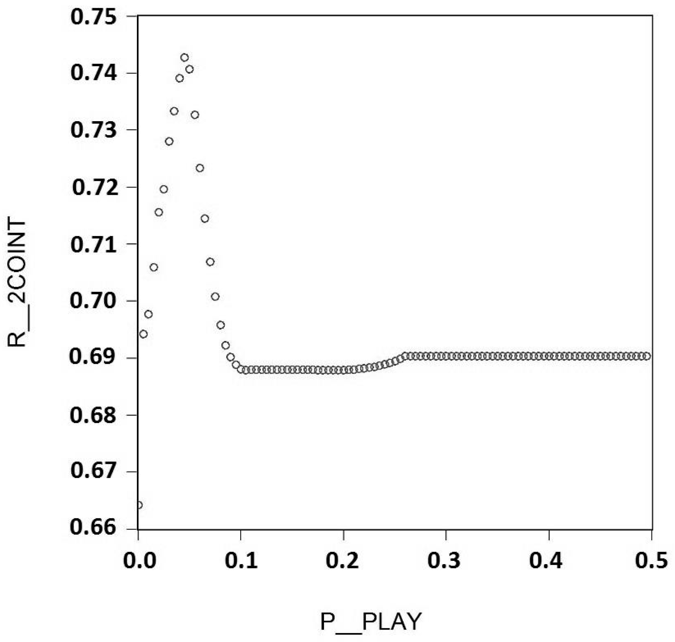
In the case of a constant play area, the key question is how to determine the area’s size. The solution is a grid search algorithm. Here, we first define an interval for the possible size of the play area. The size of the interval depends on the size of the underlying variables. In this study, the exchange rate is set as the driving variable behind the development of exports. In addition, a local maximum (or minimum) exchange rate has to be set as the starting and ending point of the grid search. The algorithm for the grid search thus starts at the beginning or end of the play area that is to be determined. Within this interval, the regression described above is estimated repeatedly for different play area sizes and the coefficient of determination is computed. We chose not to use a dummy variable for the period after the start of the financial crisis—an option that is discussed in Belke et al. (2015a). Due to the close theoretical and empirical interrelationship of hysteresis and structural breaks, a dummy variable could, under some circumstances, make it impossible to adequately capture the hysteretic aspect. This is also discussed in Belke et al. (2015a, pp. 47–50). In Figure 1, an example is provided showing the result of a grid search for Belgian exports in machinery and transport equipment (Standard International Trade Classification (SITC) 7). Here, we clearly see the constant play area maximizing the coefficient of determination.

The resulting play area and the real exchange rate enable us to compute the spurt variable. The spurt variable indicates by how much the exchange rate exceeds the play area.

The procedure is similar with a variable play area. The difference lies in the fact that the size of the play area consists not only of a constant component but also of an uncertainty variable. The play area is therefore determined using the following formula:

$$\gamma =y\left(c\right)+y\left(v\right)\times \mu$$

(2)

The variable used to model uncertainty thus enters into the regression in the form of a multiplier. This results in not just one but two components that have to be determined through grid search, in contrast to the case of constant hysteresis dynamics. This means that an interval also has to be determined for the multiplier of the uncertainty variable y(v). Its size does not depend on the exchange rate, but on the time series assigned to the multiplier. The difficulty lies in the choice of a variable that adequately represents economic uncertainty. It is a key condition that the selected variable is stationary. If a time series with a unit root is used, this leads to play area that constantly increases in size over time. This can limit the scope for interpreting the estimation results.

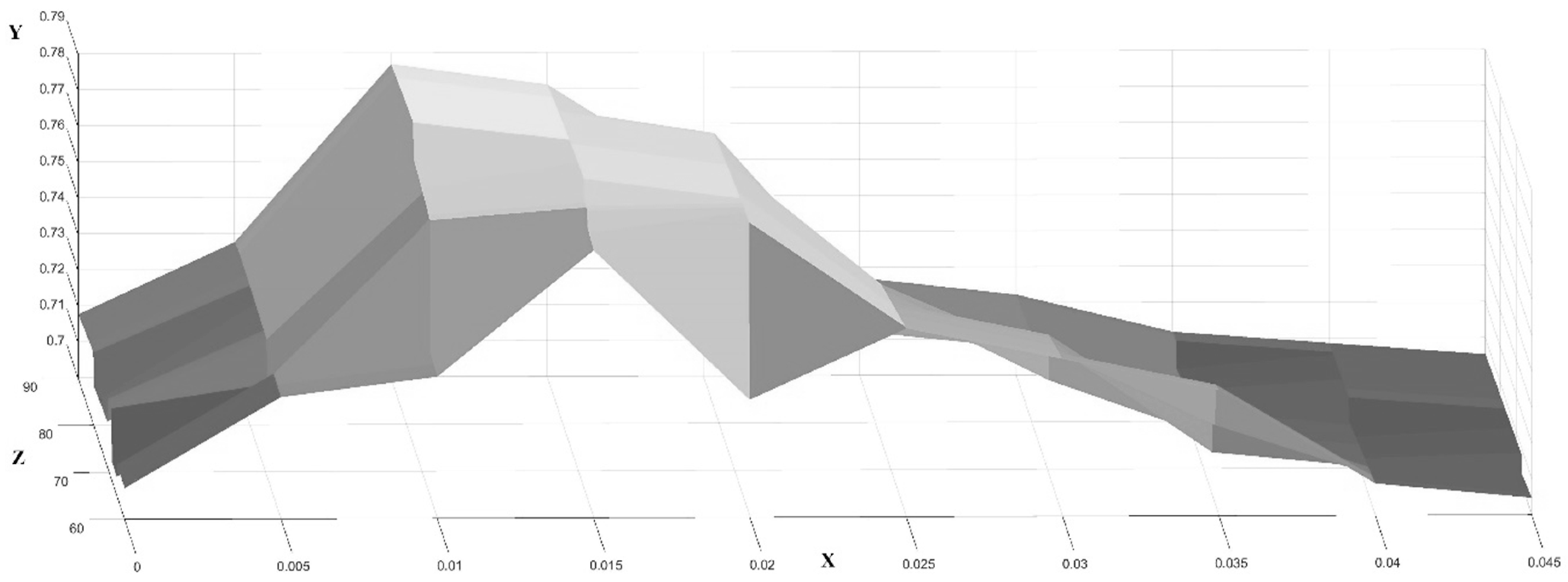
Since two, rather than just one, components must be determined by grid search in the case of hysteresis with a variable play area, the analysis has become more complex. A one-dimensional representation like Figure 1 is no longer adequate, since there is now a multitude of possible combinations of y(c) and y(v). The result is a correspondingly large matrix of coefficients of determination. To visualize this more clearly, Figure 2 presents the results of the grid search for a variable play area.

Figure 2 focuses on SITC7 exports from Belgium to the United Kingdom. Exchange rate volatility of the real exchange rate is used to model uncertainty. As expected, similarities to Figure 1 are apparent. This is especially the case when looking solely at the axes for the constant play area and the coefficient of determination.

In addition to the version with a play area including one variable component, it is also possible to include two variables to model uncertainty. Here, we forego use of the constant play component in order to still be able to limit the grid search to a two-dimensional area. The play area is computed in this case as follows:

$$\gamma =y\left(v\right)\times \mu +y\left(v2\right)\times \mu \left(2\right)$$

(3)

5. Data

In the following, we describe the data used in this study of trade relations between the United Kingdom and the European Union. The data are monthly unless otherwise noted.

The export series come from Eurostat (2017a) and are price-adjusted using a GDP deflator from the Organisation for Economic Co-operation and Development (OECD 2017a) This classification allows for differentiated examination of the influences on different categories of export products, in contrast to studies focusing solely on a country’s total exports. The focus here is on the product groups in SITC 5-8. One reason for this choice is the heterogeneity of SITC groups 0-4, which can lead to distortions in the analysis of hysteretic effects (Belke and Kronen 2015). Product groups 6 (manufactured goods) and 7 (machinery and transport equipment), in contrast, are particularly well suited to our purposes. Belke and Kronen (2015) also noted in their paper that the data on the product group SITC 8 proved unreliable. This is probably due in part to the extreme heterogeneity of the goods subsumed under this group (various types of manufactured goods, sanitary equipment, shoes, photographic equipment, clothing, etc.). One could also argue that sunk costs play a major role in the majority of these products, which again provides an argument for hysteresis. Furthermore, although a wide variety of product types are grouped together within this category, brand effects may well play a role in many of these products—as is the case in the automotive sector—but particularly for clothing and shoes. For the sake of completeness, we present the results for all product groups. We also include the product group SITC 9, which includes monetary transactions, as well as products that do not fit into the other categories. Due to the mixed composition of SITC 9, the results for goods in this group are difficult to interpret. The countries’ individual export sectors are structured differently in key respects—for instance, in terms of tolerance of uncertainty and sunk costs. This is reflected in the results.

The key dependent variable is the real bilateral exchange rate, expressed as an indirect quotation based on Eurostat (2017b) data, that is, in pounds per euro. The Consumer Price Index was used as a deflator (OECD 2017b).

GDP figures are made available at most on a quarterly basis. They are also published at a significant delay. For this reason, we used industrial production (Eurostat 2017c).

To estimate hysteretic effects with a variable play area, we used the volatility of the real exchange rate. As our estimation method, we used the standard deviation of monthly exchange rates. This variable is therefore of an exclusively economic nature and indirectly incorporates the current political and social mood. The EPUI offers an alternative (Baker et al. 2016). This index provides a measure of economic uncertainty by analyzing two newspapers per country. For Germany, they used the Handelsblatt and the Frankfurter Allgemeine Zeitung.5 The analysis is based on the number of articles published per month containing previously specified keywords that indicate uncertainty, normalized by the total number of articles published in the respective month. A measure of this kind may be subject to subjective distortions, however, as it is heavily dependent on the choice of keywords and the media culture of the particular country. The limitation to just two newspapers also means that the index can only roughly reflect the perceived economic uncertainty, since other important newspapers are left out. The advantage of using the EPUI, however, is that it allows us to not only focus on economic-level information, but also to include the media level. Since the media contribute significantly to public opinion formation, they are likely to affect export performance. However, there are no corresponding time series of the index available for Belgium, and in the case of the Netherlands, time series are only available as of 2003. The EPUI for the Netherlands is also constructed differently than those for Germany, France, and Italy. For these reasons, a general EPUI is used for the European Union as a whole to guarantee a certain level of comparability in results. The index for Europe is comprised of the individual indices for Germany, France, Italy, Spain, and the United Kingdom and is therefore not optimal for modeling uncertainty, especially in the cases of the Netherlands and Belgium. It does, however, provide a rough indicator. Another option is to look at the stock market as an indicator of economic uncertainty. The difficulty in this approach lies in the choice of an appropriate stock index. In this paper, we used the Euro Stoxx 50. It contains fifty of the largest companies listed on the stock market across all of Europe. To model uncertainty, we computed the volatility in mean monthly stock prices, that is, the mean of the highest and lowest monthly prices (Börse-Online 2017).

In this study, we also test whether the Treasury Bill EuroDollar Difference (TED-spread) spread could serve as an indicator for economic uncertainty in Europe as well (Federal Reserve Bank of Saint Louis 2017). It is defined as the difference between the three-month London Interbank Offered Rate (LIBOR) (based on the US dollar) and interest on three-month United States government bonds. Since the LIBOR gives the average interbank interest rate, the TED spread offers a more promising indicator of uncertainty in the banking sector.

The countries in this study were selected based on the intensity of their trade relations with the United Kingdom. We looked at Belgium, Germany, France, Italy, and the Netherlands. In this paper, we had all data for the relevant variables up to April 2016. Limiting our regression timeframe to the time before Brexit, from 1998 up to the beginning of 2016 has the additional benefit of allowing us to look at the export marketing independently from recent distortions caused by Brexit.

6. Results

The regressions conducted here suggest that hysteresis plays a major role in European exports. Particularly the specifications that included exchange rate volatility or Euro Stoxx 50 volatility delivered results that can be interpreted well. This is not true, however, in the case of British exports. There, even the basic models with a constant play area give little indication of a systematic influence of hysteresis on British exports to Europe. Instead, due to the financial crisis, the results often resemble structural breaks. For this reason, we concentrate in the following on evaluating the results for European exports to the United Kingdom.

The results are heavily dependent on the specification chosen in each case. It is, therefore, important to make as careful a selection as possible to provide the basis for robust conclusions. In this study, we used several different approaches. The indicators examined here—exchange rate volatility, EPUI, Euro Stoxx 50, and the TED spread—cover various aspects of uncertainty. When modeling uncertainty, it is particularly important to:

• Avoid the reduction of the spurt variable into a dummy variable for a structural break.6
• Avoid cases in which the play area is represented only by a constant despite a variable component.

This makes it clear that the EPUI and the TED spread can only be seen to a limited extent as valid indicators, at least when used in isolation as uncertainty variables. The TED spread delivered extremely inconsistent results. Exchange rate volatility and the Euro Stoxx 50 proved to be much better alternatives. For exchange rate volatility, only in two cases did we find indications of a structural break dummy. Such indications did appear, however, for exports in SITC 0 and 1, for which hysteresis is generally of low relevance. Results were similar for the Euro Stoxx 50; in fact, there, we found only one of the aforementioned problems in the case of Dutch exports in SITC 8. In addition to the specifications in which we used one variable to model uncertainty, we also tested an alternative with a play area consisting of two variable components: exchange rate volatility and EPUI. This proved to be the best of the options tested here, since structural breaks only appeared for French exports in SITC 1. This makes it easier to distinguish between the existence of a structural break and actual hysteretic effects. Especially when using a constant play area and to some extent with other specifications as well, we found substantially more cases in which the play area was only passed in one direction (an indication for a structural break instead of hysteresis). In addition, it accounts for two different aspects of uncertainty, a clear advantage over the previous specifications.

Table 1. Results for the regressions with a variable play area (estimated using exchange rate volatility and European EPUI).

	SICT Product Groups
	0	1	2	3	4	5	6	7	8	9	Total
BE	α = 1.92 × 108 ***	α = −45136055 ***	α = −33460314 ***	α = 7.96 × 108 ***	α = −45633528 ***	α = 5.07 × 108**	α = −5.06 × 108 ***	α = 2.43 × 108	α = −43864590	α = 5.63 × 108 ***	α = −1.67 × 108
	p(α) = 0.0000	p(α) = 0.0000	p(α) = −33460314	p(α) = 0.0022	p(α) = 0.0022	p(α) = 0.0116	p(α) = 0.0000	p(α) = 0.2424	p(α) = 0.4810	p(α) = 0.0000	p(α) = 0.6702
	γ(v) = 0.000200	γ(v) = 0.000000	γ(v) = 0.001100	γ(v) = 0.000000	γ(v) = 0.000000	γ(v) = 0.000100	γ(v) = 0.000500	γ(v) = 0.000200	γ(v) = 0.000200	γ(v) = 0.000100	γ(v) = 0.000200
	γ(v2) = 3.000000	γ(v2) = 184.0000	γ(v2) = 0.800000	γ(v2) = 13.80000	γ(v2) = 3.000000	γ(v2) = 3.000000	γ(v2) = 106.0000	γ(v2) = 62.00000	γ(v2) = 33.00000	γ(v2) = 2.000000	γ(v2) = 56.00000
	β = −2.50 × 108 ***	β = −32277771 ***	β = 38845417 ***	β = −8.97 × 108 ***	β = 72315272 ***	β = −9.53 × 108 ***	β = 3.33 × 108 ***	β = −2.09 × 109 ***	β = −4.86 × 108 ***	β = −6.86 × 108 ***	β = −3.32 × 109 ***
	p(β) = 0.0000	p(β) = 0.0000	p(β) = 0.0001	p(β) = 0.0008	p(β) = 0.0000	p(β) = 0.0000	p(β) = 0.0000	p(β) = 0.0000	p(β) = 0.0000	p(β) = 0.0000	p(β) = 0.0000
GE	α = 93822114 ***	α = −35351857 ***	α = −1.39 × 108 ***	α = −6.31 × 108 ***	α = −75102201 ***	α = −4.52 × 108**	α = −2.35 × 108 ***	α = −2.83 × 109 ***	α = 9.20 × 108 ***	α = −1.06 × 109 ***	α = −2.20 × 109 ***
	p(α) = 0.0001	p(α) = 0.0006	p(α) = 0.0009	p(α) = 0.0000	p(α) = 0.0000	p(α) = 0.0118	p(α) = 0.0005	p(α) = 0.0000	p(α) = 0.0000	p(α) = 0.0000	p(α) = 0.0008
	γ(v) = 0.000100	γ(v) = 0.001300	γ(v) = 0.000000	γ(v) = 0.000200	γ(v) = 0.000100	γ(v) = 0.000400	γ(v) = 0.001400	γ(v) = 0.001300	γ(v) = 0.000200	γ(v) = 0.000100	γ(v) = 0.000600
	γ(v2) = 275.0000	γ(v2) = 3.000000	γ(v2) = 2.000000	γ(v2) = 10.00000	γ(v2) = 3.000000	γ(v2) = 62.00000	γ(v2) = 88.00000	γ(v2) = 0.000000	γ(v2) = 3.000000	γ(v2) = 4.000000	γ(v2) = 4.000000
	β = −2.44 × 108 ***	β = 48896285 ***	β = 1.30 × 108 ***	β = 6.85 × 108 ***	β = 76972857 ***	β = −8.81 × 108 ***	β = −6.87 × 108 ***	β = −3.77 × 109 ***	β = −1.23 × 109 ***	β = 1.20 × 109 ***	β = −6.32 × 109 ***
	p(β) = 0.0000	p(β) = 0.0018	p(β) = 0.0022	p(β) = 0.0000	p(β) = 0.0000	p(β) = 0.0000	p(β) = 0.0000	p(β) = 0.0000	p(β) = 0.0000	p(β) = 0.0000	p(β) = 0.0000
FR	α = −3.75 × 108	α = 33610219	α = 47907338	α = −3.42 × 108	α = −20157929	α = −2.07 × 108	α = 2.02 × 108	α = −9.60 × 108	α = −1.48 × 108	α = 3.01 × 108	α = −9.90 × 108
	p(α) = 0.0000	p(α) = 0.0935	p(α) = 0.0991	p(α) = 0.0021	p(α) = 0.0004	p(α) = 0.0006	p(α) = 0.0283	p(α) = 0.0516	p(α) = 0.0216	p(α) = 0.0000	p(α) = 0.1089
	γ(v) = 0.000000	γ(v) = 0.001700	γ(v) = 0.000100	γ(v) = 0.000000	γ(v) = 0.001200	γ(v) = 0.001300	γ(v) = 0.000000	γ(v) = 0.000500	γ(v) = 0.000500	γ(v) = 0.000000	γ(v) = 0.000500
	γ(v2) = 3.000000	γ(v2) = 7.800000	γ(v2) = 3.100000	γ(v2) = 3.000000	γ(v2) = 1.000000	γ(v2) = 13.00000	γ(v2) = 5.200000	γ(v2) = 18.00000	γ(v2) = 14.00000	γ(v2) = 3.000000	γ(v2) = 7.000000
	β = 2.75 × 108	β = −2.69× 108	β = −77572526	β = 8.20 × 108	β = 72167564	β = −5.57 × 108	β = −4.17 × 108	β = −1.90 × 109	β = −5.08 × 108	β = −3.12 × 108	β = −2.75 × 109
	p(β) = 0.0000	p(β) = 0.0000	p(β) = 0.0128	p(β) = 0.0000	p(β) = 0.0000	p(β) = 0.0000	p(β) = 0.0006	p(β) = 0.0007	p(β) = 0.0000	p(β) = 0.0000	p(β) = 0.0003
IT	α = 1.11 × 108	α = −8355379	α = 45631207	α = −1.65 × 108	α = −12536134	α = −75446519	α = −4.98 × 108	α = −4.29 × 108	α = 62332150	α = 9.05 × 108	α = −1.10 × 109
	p(α) = 0.0000	p(α) = 0.5523	p(α) = 0.0027	p(α) = 0.0323	p(α) = 0.0877	p(α) = 0.0017	p(α) = 0.0000	p(α) = 0.0016	p(α) = 0.3307	p(α) = 0.0248	p(α) = 0.0000
	γ(v) = 0.000100	γ(v) = 0.000100	γ(v) = 0.000000	γ(v) = 0.000100	γ(v) = 0.000100	γ(v) = 0.001300	γ(v) = 0.000000	γ(v) = 0.000700	γ(v) = 0.000500	γ(v) = 5.00 × 10−5	γ(v) = 0.001300
	γ(v2) = 8.000000	γ(v2) = 95.00000	γ(v2) = 2.500000	γ(v2) = 2.000000	γ(v2) = 0.000100	γ(v2) = 9.000000	γ(v2) = 14.50000	γ(v2) = 14.00000	γ(v2) = 16.00000	γ(v2) = 0.600000	γ(v2) = 9.000000
	β = −1.46 × 108	β = −47640379	β = −57588745	β = 2.19 × 108	β = 18373368	β = −3.39 × 108	β = 4.42 × 108	β = −3.48 × 108	β = −7.34 × 108	β = −9.12 × 108	β = −1.52 × 109
	p(β) = 0.0000	p(β) = 0.0022	p(β) = 0.0005	p(β) = 0.0052	p(β) = 0.0094	p(β) = 0.0000	p(β) = 0.0000	p(β) = 0.0452	p(β) = 0.0000	p(β) = 0.0278	p(β) = 0.0000
NL	α = 2.78 × 108	α = 38605586	α = 2.94 × 108	α = −25374134	α = 1.70 × 108	α = −3.53 × 108	α = −26871777	α = −1.95 × 108	α = −36321946	α = 56192718	α = 7.13 × 108
	p(α) = 0.0000	p(α) = 0.0041	p(α) = 0.0000	p(α) = 0.8458	p(α) = 0.0000	p(α) = 0.0144	p(α) = 0.5284	p(α) = 0.4473	p(α) = 0.6730	p(α) = 0.0003	p(α) = 0.2025
	γ(v) = 0.000000	γ(v) = 0.000300	γ(v) = 0.000000	γ(v) = 0.000800	γ(v) = 0.000300	γ(v) = 0.000900	γ(v) = 0.000300	γ(v) = 0.000000	γ(v) = 0.000300	γ(v) = 0.000200	γ(v) = 0.000300
	γ(v2) = 28.00000	γ(v2) = 46.00000	γ(v2) = 67.00000	γ(v2) = 35.00000	γ(v2) = 61.00000	γ(v2) = 12.00000	γ(v2) = 46.00000	γ(v2) = 24.00000	γ(v2) = 10.00000	γ(v2) = 56.00000	γ(v2) = 20.00000
	β = −4.65 × 108	β = −87889369	β = −3.34 × 108	β = 1.05 × 109	β = −96635944	β = −7.69 × 108	β = −2.74 × 108	β = −1.99 × 109	β = −5.32 × 108	β = −2.27 × 108	β = −4.09 × 109
	p(β) = 0.0000	p(β) = 0.0000	p(β) = 0.0000	p(β) = 0.0000	p(β) = 0.0000	p(β) = 0.0001	p(β) = 0.0000	p(β) = 0.0000	p(β) = 0.0000	p(β) = 0.0000	p(β) = 0.0000

Two variables for modeling uncertainty: y(v) is the multiplier for exchange rate volatility and y(v2) is the multiplier for European Economic Policy Uncertainty Index (EPUI). Instructions on how to read this table and the tables in the Appendix: The results in which both the coefficient and the grid search correspond to theoretical expectations and the results are significant at the 5% level are shown in bold. All cases in which the coefficient for the original exchange rate variable does not correspond to theoretical expectations and is significant at the 5% level are shown in italics. Red signifies that the play area is too large for the hysteresis loop to be passed through completely. Results in which the play area is limited to one constant are shown in gray. Level of significance: *** for 1%, ** for 5%, *for 10%.

presents the results by countries and SITC groups. To illustrate how to interpret the results, we look at the regression results for the German exports of machinery and transport equipment (SITC 7). The coefficients for RER $(\alpha )$ and the spurt variable ($\beta$) are both negative as expected. The coefficients for $y\left(v\right)$ and $y\left(v2\right)$ determine the size of the play area (see Equation (3)). If the result is marked in red, it would indicate that the resulting play area is too large for the exports to have shown an upwards and downwards spurt movement. If only a one-sided spurt movement could be observed, it could very well point to a simple structural break. As this is not the case in this example, the results show significant evidence for hysteresis.

Substantial differences are evident between SITC groups 0–4 and 5–8. In the former, the results are highly disparate and give little indication of hysteresis. In the latter groups, this is not true; almost across the board, there are strong indications of hysteresis as a driving factor. The same can be said for the aggregated exports.

The results for Italy are particularly noteworthy. They serve as a striking example of how substantially the selected modeling of uncertainty can influence the results. With the exception of the estimation of the Euro Stoxx 50, the various other specifications provided mostly mixed indications of hysteresis as a driving force in export dynamics (see Appendix A). In contrast, when estimating a combination of exchange rate volatility and the EPUI, the results give strong indications of hysteretic effects. This is an indication that the interaction between these two components plays a substantially more important role than each component viewed in isolation. With the other specifications, either the results for SITC 5 (as an example) were indicators of a structural break, or the exchange rate variable used originally or the movement within the play area had a coefficient with a positive sign. In this case, however, hysteresis appears to be relevant as a driving force in export dynamics.7 A similar observation can be made for the results for the aggregated exports of Italy. The analysis here is limited to this brief examination of the model with two indicators of uncertainty. All other analyses are presented in the Appendix A.

The question still remains, however, as to whether the combination of uncertainty variables selected here is the best choice. The fact that this kind of play area encompasses media and public perceptions as well as a primarily economic perspective in the form of exchange rate volatility speaks in favor of the version used here.

It is difficult to predict what impacts the pound’s devaluation will have in the months and years to come. For this reason, research should examine whether the depreciation of the pound against the euro has already led to a spurt in European exports to the United Kingdom.

Table 2. Spurt movements between January and April 2016.

Spurt Movements Since January 2016	Country	SITC Product Groups
		5	6	7	8	TOTAL
Constant	Belgium	−	−	↑	↑	↑
	Germany	−	−	−	−	−
	France	−	−	↑	↑	↑
	Italy	−	−	−	−	↑
	Netherlands	−	−	↑	↑	↑
Exchange rate volatility	Belgium	↑	−	−	−	−
	Germany	↑	−	−	↑	−
	France	↑	↑	↑	−	↑
	Italy	−	↑	↑	−	−
	Netherlands	−	−	↑	↑	↑
EPUI	Belgium	−	−	↑	−	↑
	Germany	−	−	−	−	−
	France	−	−	↑	−	−
	Italy	−	↑	−	−	−
	Netherlands	−	−	−	↑	−
Euro Stoxx 50	Belgium	↑	↑	−	−	−
	Germany	−	−	−	↑	↑
	France	−	↑	↑	−	−
	Italy	−	−	−	−	−
	Netherlands	−	−	−	↑	−
TED Spread	Belgium	−	−	↑	↑	↑
	Germany	↑	−	−	−	−
	France	↑	−	↑	↑	↑
	Italy	↑	−	↑	−	↑
	Netherlands	−	−	↑	↑	↑
Exchange rate volatility + EPUI	Belgium	↑	−	−	−	−
	Germany	−	−	−	↑	−
	France	−	↑	−	−	−
	Italy	−	↑	−	−	−
	Netherlands	−	−	↑	−	−

↑ symbolizes an upward spurt; − no change in the spurt variable. Grey areas indicate a result that corresponds to the theory of hysteresis (both for the play variable and for the spurt variable), together with significance at the 5% level. Exchange rate volatility + EPUI relate to the results for European EPUI. An upward spurt means a decline in exports to the United Kingdom. SITC: Standard International Trade Classification.

shows whether the respective spurt variable had already reacted to the depreciation of the pound against the euro in the period January to April 2016,8 that is, shortly before the referendum.9 This mode of presentation also allows for comparison of the play areas and their respective effects on the development of the spurt variables in the different specifications, despite the different sizes of the multipliers. The selected presentation comprises all of the specifications used in this study in order to provide as complete a picture as possible, because the results depend on the variable selected to model uncertainty. In addition, we only include the product groups in SITC 5–8, as well as aggregated exports, as we found that these were the groups with the greatest hysteretic effect.

For aggregated exports of the various countries, spurt variables already showed a reaction in 7 out of 30 cases. This was not the case, however, in 16 out of 30 cases.10 With regard to the individual product groups, no clear pattern can be identified with regard to whether certain categories reacted more than others. The results for regressions using EPUI are clear, however, and generally show no change over the period under observation here (in the sense of a reaction of the spurt variable). The case is similar for the specification with two uncertainty variables. Here the results show a relatively large number of spurt movements already in progress, but with a constant play area. The reason for this is that estimations with a constant play area lead to the play area not reacting to phases with differing levels of uncertainty but instead always having the same threshold. This means that a major devaluation of the pound, as seen at the end of 2015, will lead to a faster change in the spurt variable. With a variable play area, this takes place more slowly, since the play area adapts to the change.

For the majority of product groups in SITC 5–8 and aggregated exports, the results give significant indications of hysteresis, which therefore apparently plays an important role in European exports to the United Kingdom. At the same time, the evidence that exports have already begun to react (in the sense of a decline in exports due to a less advantageous exchange rate) is more mixed. Against this backdrop, one can expect a more dramatic drop in European exports in the future if the pound continues to depreciate. At the moment, the effects of Brexit on the exchange rate and on exports are still within the bounds of the play area. This can be traced back, first, to the option value of waiting. Second, the time period defined in Table 2 is fairly narrow (January to April 2016). Over such a limited period, companies can protect themselves relatively well against losses due to exchange rate fluctuations through hedging and other safeguarding mechanisms. Both of these explanations for European exports’ weak reaction at present are specific to the limited period of time under consideration here. How the British pound will fare in the future, and how negotiations over future trade agreements will go, should therefore be considered critical factors.

7. Conclusions and Perspectives

This study applied a variety of approaches to modeling economic uncertainty in a first attempt to determine the influence of hysteresis. This provides the basis, at minimum, for a limited comparison of the models’ results. The results show that hysteresis is currently having little effect on British exports to the European Union. However, across all specifications, the results show that hysteresis is having a substantial impact on exports from Belgium, Germany, France, Italy, and the Netherlands to the United Kingdom.

In addition to the indicators of uncertainty used by e.g., Belke et al. (2015a) or Belke and Kronen (2015) (exchange rate volatility or the EPUI), the present study also tested the validity of stock indices and the TED spread in modeling uncertainty. Our focus was on European exports. Stock indices—here, the Euro Stoxx 50—proved appropriate as alternatives to exchange rate volatility or the EPUI. This approach could conceivably be extended further by creating individual stock indices for each of the countries under examination to eliminate distortions. The TED spread produced extremely mixed results and therefore appears less appropriate as an index. A possible alternative would be to repeat the estimation with a European version of the TED spread. We also used two uncertainty variables to represent uncertainty. This has the advantage of covering multiple aspects of economic uncertainty. Since exchange rate volatility and the EPUI were combined in the present study—to link this research to the existing literature, among other reasons—it appears promising to explore further possibilities. As discussed above, exchange rate volatility, stock indices, and combined play areas with multiple uncertainty variables appear to produce the most clearly interpretable results. A combination of exchange rate volatility and an indicator for uncertainty on the stock market could potentially offer useful insights.

A further study of this kind should be conducted at a later point in time. It is not yet clear how Brexit will unfold in its entirety, how the process will be negotiated and managed, and what influences it will have on trade relations between the United Kingdom and Europe. It is, therefore, possible that future analyses of the trade relations examined here will arrive at different conclusions. This will be particularly interesting to see in the cases where the play area under examination was so large that the hysteresis loop was not passed through completely during the period covered. In addition, the fundamental effect of a weaker British pound—in the sense of increasing British exports11 and declining European imports—could possibly counteract higher trade barriers resulting from a “hard” Brexit.

References

- Agur, Itai. 2003. Trade-volume Hysteresis: An Investigation Using Aggregate Data. Research Memorandum WO No. 740. Amsterdam, The Netherlands: Research Department, De Nederlandsche Bank NV. [Google Scholar]
- Baker, Scott R., Nick Bloom, and Steven J. Davis. 2016. Economic Political Uncertainty. Available online: http://www.policyuncertainty.com/index.html (accessed on 19 December 2016).
- Baldwin, Richard, and Paul Krugman. 1989. Persistent Trade Effects of Large Exchange Rate Shocks. The Quarterly Journal of Economics 104: 635–54. [Google Scholar] [CrossRef]
- Belke, Ansgar, and Dominik Kronen. 2015. Exchange Rate Bands of Inaction and Play-Hysteresis in Greek Exports to the Euro Area, the US and Turkey: Sectoral Evidence. Empirica 43: 349–90. [Google Scholar] [CrossRef]
- Belke, Ansgar, and Thorsten Polleit. 2009. Monetary Economics in Globalised Financial Markets. Heidelberg: Springer-Verlag. [Google Scholar]
- Belke, Ansgar, and Ulrich Volz. 2015. The Strong Euro Challenges for the European Central Bank and Implications for the Global Economy. AEI Insights 1: 53–68. [Google Scholar]
- Belke, Ansgar, Matthias Göcke, and Martin Günther. 2013. Exchange Rate Bands of Inaction and Play-Hysteresis in German Exports—Sectoral Evidence for Some OECD Destinations. Metroeconomica 64: 152–79. [Google Scholar] [CrossRef]
- Belke, Ansgar, Matthias Göcke, and Laura Werner. 2014. Hysteresis Effects in Economics—Different Methods for Describing Economic Path-dependence. In Hysteresis—Types, Applications and Behavior Patterns in Complex Systems. Edited by José Carlos Dias. New York: Nova Publishers, pp. 19–42. [Google Scholar] [CrossRef]
- Belke, Ansgar, Matthias Göcke, and Laura Werner. 2015a. Exchange Rate Volatility and other Determinants of Hysteresis in Exports—Empirical Evidence for the Euro Area. Review of Economic Analysis 7: 25–53. [Google Scholar]
- Belke, Ansgar, Anne Oeking, and Ralph Setzer. 2015b. Domestic Demand, Capacity Constraints and Exporting Dynamics: Empirical Evidence for Vulnerable Euro Area Countries. Economic Modelling 48: 315–25. [Google Scholar] [CrossRef]
- Bertelsmann-Stiftung. 2016. Fokuspapier. Die Folgen eines Brexit aus der Sicht Deutscher und Britischer Unternehmen. Available online: https://www.bertelsmann-stiftung.de/fileadmin/files/BSt/Publikationen/GrauePublikationen/NW_Brexit-2016_DE.pdf (accessed on 8 August 2018).
- Börse-Online. 2017. Historische Kursdaten für EURO STOXX 50. Available online: http://www.boerse-online.de/index/historisch/Euro_Stoxx_50 (accessed on 12 May 2017).
- Cameron, David. 2013. EU Speech at Bloomberg. Available online: https://www.gov.uk/government/speeches/eu-speech-at-bloomberg (accessed on 9 July 2017).
- Campa, José Manuel. 2004. Exchange Rates and Trade: How Important Is Hysteresis in Trade. European Economic Review 48: 527–48. [Google Scholar] [CrossRef]
- Côté, Agathe. 1994. Exchange Rate Volatility and Trade: A Survey. Working Paper 94-5, International Department, Bank of Canada Ottawa, Ottawa, ON, Canada. Available online: https://www.bankofcanada.ca/wp-content/uploads/2010/04/wp94-5.pdf (accessed on 12 May 2017).
- De Grauwe, Paul. 2016. Economics of Monetary Union. New York: Oxford University Press. [Google Scholar]
- Dixit, Avinash. 1989. Entry and Exit Decisions under Uncertainty. Journal of Political Economy 97: 620–38. [Google Scholar] [CrossRef]
- Eurostat. 2017a. EU Handel nach SITC seit 1988 (DS-018995). Available online: https://data.europa.eu/euodp/de/data/dataset/PNtLrEMxMmcWouzaCbJSg (accessed on 8 August 2017).
- Eurostat. 2017b. Euro/Ecu-Wechselkurse—Monatliche Daten. Available online: http://appsso.eurostat.ec.europa.eu/nui/show.do?dataset=ert_bil_eur_m&lang=de (accessed on 12 May 2017).
- Eurostat. 2017c. Produktion in der Industrie—Monatliche Daten. Available online: http://appsso.eurostat.ec.europa.eu/nui/show.do?dataset=sts_inpr_m&lang=de (accessed on 12 May 2017).
- Federal Reserve Bank of Saint Louis. 2017. TED Spread (TEDRATE). Available online: https://fred.stlouisfed.org/series/TEDRATE (accessed on 12 May 2017).
- Fedoseeva, Svetlana, and Laura Werner. 2014. Asymmetry and Hysteresis: Two Perspectives on Pricing-to-Market Nonlinearity. Working Paper 2014.02, International Network for Economic Research, Cologne, Germany. Available online: www.infer-research.eu/en/publications/download/40 (accessed on 12 May 2017).
- Ilmakunnas, Pekka, and Satu Nurmi. 2010. Dynamics of Export Market Entry and Exit. The Scandinavian Journal of Economics 112: 101–26. [Google Scholar] [CrossRef]
- Impulitti, Giammario, Alfonso A. Irarrazabal, and Luca David Opromolla. 2013. A Theory of Entry into and Exit from Export Markets. Journal of International Economics 90: 75–90. [Google Scholar] [CrossRef]
- Kannebley, Sérgio, Jr. 2008. Tests for the Hysteresis Hypothesis in Brazilian Industrialized Exports. A threshold cointegration analysis. Economic Modelling 252: 171–90. [Google Scholar] [CrossRef]
- Máñez, Juan A., María E. Rochina-Barrachina, and Juan A. Sanchis. 2008. Sunk Costs Hysteresis in Spanish Manufacturing Exports. Review of World Economics 144: 272–94. [Google Scholar] [CrossRef]
- OECD. 2017a. Economic Outlook No. 102. November 2017: GDP Deflators, Forecast Growth. Available online: http://stats.oecd.org/Index.aspx?QueryId=61354# (accessed on 12 May 2017).
- OECD. 2017b. Inflation (CPI). Available online: https://data.oecd.org/price/inflation-cpi.htm (accessed on 12 May 2017).