The Role of Canceled Warrants in the LME Market

Abstract

This article visits the question of whether canceled warrants (CWs) have a positive effect on LME metal prices. To examine this question carefully, a regression model is applied. This paper finds a statistically significant positive link between CWs and LME metal prices, including aluminum, zinc, tin, and nickel. However, other metals such as copper and lead are not statistically significant. The second objective of the study is to identify the dynamic response of metal price returns for aluminum, zinc, tin, and nickel to an innovation in the CWs using VAR. It is found that the positive impact of the CWs on metal returns is transitory.

1. Introduction

High cyclical fluctuations in commodity prices, with somewhat severe volatilities, have brought about a debate over the developments occurring in commodity markets (Singleton 2014). Recent years have seen a rapid growth in the participation of investors in the commodity market, in what is being called the ‘financialization’ of commodity markets (Cheng and Xiong 2014). This phenomenon has occurred where the commodity markets have become important, as institutional investors have come to regard commodities as an alternative asset class (Park 2019). Tang and Xiong (2012) concluded that the financialization of commodity markets through institutional investors’ index funds has significantly impacted market dynamics and volatilities in commodity markets.

The LME (London Metal Exchange)1 is the world’s largest futures exchange in the metal industry, including for six base metals—copper, aluminum, lead, zinc, tin, and nickel—and is known for being quite correlated with the business cycle (Park 2018). Based on Bloomberg data, the LME is truly a global commodity exchange, as 95% of trades originate from overseas.

Producers of commodities do not have direct contract with the consumers who use their commodities in business activities (Otani 1983). The place for transactions of inventory stock between producers and consumers exists with middlemen, who deliver commodities from producers to consumers. Otani (1983) argued that the LME might be the most famous inventory stock market using its own warehouse system. Traders in LME can take physical deliveries of metals and sell excess inventory of over-supply in the market, which is possible due to peculiar LME warehouse regulations. There are more than 690 warehouses and storage facilities worldwide which are licensed by an LME authority. On a daily basis, LME reports the availability of the six base metal inventory at each of these warehouses. Most global sell-side brokers, such as Goldman Sachs, Macquarie and Societe Generale, report the variation of canceled warrants (CWs) in the LME market to focus on market trading momentum as a key factor.

The Metal Bulletin points out that “CWs2 are important in that they represent the change in stockpiles of metal that may no longer be available at LME warehouses, and which are booked for removal or onward shipment. This information is an indicator of physical demand”. Metals on warrants represent inventories in store at the LME’s warehouse, while CWs imply metal earmarked for physical delivery soon. Investors cancel their warrants because they want to take it out of the LME warehouse. This is important signal for market demand/supply fundamentals. A rise in CWs suggests stronger market demand for the LME metals, and deliveries thereof. A warehouse inventory is the significant barometer to investors,3 and there is an inverse relationship between inventories and prices as movement in stocks affect the future price direction. A sharp decline in inventories implies the demand is rising with less supply.

Table 1. Possible relationship between the CW ratio and effect on the metal price.

Inventories	CW Ratio	Effect on Metal Price
Up	Down	Negative
Down	Up	Positive

Note: the inverse relationship between inventories and CWs is held due to the definition of the CW calculation.

exhibits the possible stylized fact, which relates to dynamics between the CW ratio direction and the metal price direction. A rise in warehouse stocks or fall in the CW ratio suggests a negative direction for metal prices, while a fall in the inventory or rise in the CW ratio implies a positive trend for metal prices.

Investors may want to cancel their warrants because they take it out of the authorized LME warehouse to squeeze the market spread. These sequential investors’ reactions have been strengthening through market expectation. This is possible because first, the middlemen are the commodity developers or smelters such as Glencore, Nyrstar and Rusal, and the warehouse companies such as Access World, C. Steinweg and Mitsubishi Logistics. They have a lot of market information, and are experienced professionals regarding metal market dynamics. I believe that the changes in CWs affect the investment sentiment and the financialization of the LME market. Second, the LME has very peculiar prompt dates. The LME provides spot (cash), futures (three month; benchmark) and various option contracts. The LME addresses daily rolling three month (3M) futures contracts that are different from those in other commodity markets, which are based on monthly prompt dates (Park and Lim 2018). This may convince traders, analysts, and index investors who have attributed the metal price direction to speculation that the fundamentals have indeed been improving. I develop my hypothesis as follows:

Hypothesis 1 (H1).

The rise in CWs increases the LME metal price.

I consider pairs of variables; the first of each pair is the CWs, and the second is an LME metal price movement. Unfortunately, there is no previous study in the CWs area to the best of my knowledge, even though there are quite a few in LME market dynamics, such as on testing market efficiency (Arouri et al. 2011; Otto 2011; Park and Lim 2018) and measuring market volatility (Figuerola-Ferretti and Gilbert 2008). The purpose of this paper is to test the above hypothesis using daily LME market data from January 2006 to December 2018. This study uses a regression model and finds a statistically significant link between CWs and LME metal prices, including aluminum, zinc, tin and nickel, while the other metals are not statistically significant. Using the VAR model, it is found that the impact of a CW innovation on spot returns of aluminum, zinc, tin and nickel is transitory rather than permanent.

The paper is organized as follows. Section 2 reviews the previous literature about the LME. In Section 3, I present the research model and data with a summary of statistics and unit root test. Section 4 presents the main results. In the final section, I provide the summary and conclusion.

2. Literature Review

There is no direct study of CWs in the LME, or even in other commodity markets. This section reviews the previous studies in the LME-related-area. There are three different categories within LME studies. First, the testing of LME market efficiency is an important issue. However, there has not been consensus regarding the market efficiency of the LME. Canarella and Pollard (1986) and MacDonald and Taylor (1988) found that the LME was an efficient market, while Otto (2011) and Park and Lim (2018) found opposing results. Park and Lim (2018) argued that the financialization of commodities was growing.

Second, the financialization of the LME market has been debated. Koitsiwe and Adachi (2018) found that LME real copper spot prices had been characterized by structural changes, and its determinants vary in a distinct period. They showed that financial speculation had accentuated copper price moves during the last decade. Guzman and Silva (2018) argued that, following the recent price boom, some dissent had arisen around the role played by non-fundamentals such as liquidity or money supply in major commodity markets. They found that some indications of financialization in the copper price explained the price dynamics using the VAR model. Park (2019) employed Granger causality tests to analyze the role of speculators using weekly COTR (Commitment of Traders Reports) data, and presented statistically significant evidence that the position changes of speculators, such as hedge funds, Granger-cause the prices of base metals, such as aluminum, copper and zinc among the six base metals.

Third, Figuerola-Ferretti and Gilbert (2008) studied the measurement of volatility in the LME market using realized volatility.4 They examined the spot and three month aluminum and copper volatilities. They found that both spot and three month price volatilities of aluminum and copper followed a long memory process, caused by speculative traders.5 They found no evidence that the volatilities processes were fractionally cointegrated. Park (2018) provided evidence of volatility transmission between oil and the base metals through the bivariate GARCH model. Within the results, he argued that hedging decisions across the oil and LME futures were feasible to deal with market risk. Park and Lim (2018) examined whether the price volatility of the LME changed within a sample period, to check the possibility of time-varying volatility due to the financialization of commodity markets. They showed the results from the difference-in-means tests of volatility difference in two sub-periods: pre-crisis (2000–2008) and post-crisis (2009–June 2016), which found that the LME’s volatility was somewhat larger post-crisis when compared to pre-crisis, with a statistical significance of 1% for all base metals except nickel.

3. Research Model and Data

3.1. Research Model

When examining the effect of CWs on base metal spot prices in LME, I developed a simple empirical framework. In its basic form, the following model determines the spot price returns of LME base metals with respect to CWs:

$${\mathrm{SR}}_{\mathrm{i},\mathrm{t}}={\mathsf{\beta }}_0+{\mathsf{\beta }}_1{\mathrm{CW}}_{\mathrm{i},\mathrm{t}}+{\mathsf{\epsilon }}_{\mathrm{i},\mathrm{t}}$$

(1)

where ${\mathrm{SR}}_{\mathrm{i},\mathrm{t}}$ is the natural logarithm of the spot price return of base metal i against the previous day; ${\mathrm{CW}}_{\mathrm{i},\mathrm{t}}$ is the canceled warrant on the day of base metal i in the LME market; and ${\mathsf{\epsilon }}_{\mathrm{i},\mathrm{t}}$ is the vector of independent and identically distributed (i.i.d.) errors of each of the ${\mathrm{SR}}_{\mathrm{i},\mathrm{t}}$s. If rising CWs tend to encourage the investment momentum upward, then ${\mathsf{\beta }}_1>0$ is expected. Given the fact that LME investors tend to view CWs as a key variable, commodity funds such as hedge funds and CTAs (Commodity Trading Advisors) are likely to have a significant influence on metal prices.

3.2. Data

Daily data relating to the period of January 2006 to December 2018 are used for estimating Equation (1), providing N = 3284 observations through Bloomberg. In particular, to evaluate the effect of stockpiling on metal prices, I collected the available data on the LME metal stockpile. To measure the effect of the stockpile, CWs are used.

Table 2. Summary statistics. The total observation contains 3284 obs. (3 January 2006–31 December 2018; daily data). The natural logarithm data are applied in the returns calculations. The distributions for all returns and CWs are skewed and fat-tailed, as indicated by the high significance of the Jarque–Bera test for normality.

	Variable	Mean	Standard Deviation	Skewness	Maximum	Minimum	Kurtosis	Jarque-Bera
copper	cu_cw	0.1836	0.1564	1.0898	0.6742	0.0013	3.3818	458.75 (0.00)
	cu_r	0.0002	0.0182	0.1461	0.1244	−0.0980	6.8328	307.12 (0.00)
aluminum	al_cw	0.2194	0.1821	0.3844	0.5996	0.0037	1.7159	7548.3 (0.00)
	al_r	0.0005	0.0148	−0.0069	0.0660	−0.0752	4.7523	133.47 (0.00)
lead	pb_cw	0.1827	0.1792	0.9114	0.7752	0.0004	2.6438	364.71 (0.00)
	pb_r	0.0004	0.0221	−0.0028	0.1389	−0.1236	5.8982	228.62 (0.00)
zinc	zn_cw	0.1845	0.1797	1.1336	0.7610	0.0019	3.1896	474.37 (0.00)
	zn_r	0.0003	0.0209	−0.0039	0.1046	−0.1083	4.9927	154.59 (0.00)
tin	sn_cw	0.1435	0.1283	1.3391	0.6780	0.0000	4.4941	702.47 (0.00)
	sn_r	0.0005	0.0182	0.0856	0.1663	−0.1082	9.3753	443.00 (0.00)
nickel	ni_cw	0.1840	0.1504	0.5176	0.8586	0.0029	2.4871	197.66 (0.00)
	ni_r	0.0002	0.0237	0.1358	0.1423	−0.1284	5.6834	221.95 (0.00)

presents the descriptive statistics of returns and CWs. It is found that both the returns and CWs are strongly leptokurtic. The skewness and kurtosis measures show that the returns distributions are asymmetric and fat-tailed, which is known as excess kurtosis. The standard deviation of daily log returns as the volatility over the period shows that nickel is the largest, but aluminum is the lowest. Jarque–Bera statistics in Table 2 are for checking normal distribution, and reveal no normally distributed data within the considered data set. The conclusion for the data finds that the distributions for all returns and CWs are skewed and fat-tailed.

3.3. Stationarity Check: Unit Root Tests

To test the stationarity of the variables, this paper employs the ADF (Augmented Dickey Fuller) test and Phillip–Perron (PP) test, which are given in

Table 3. Unit root test results. The sample consists of 3284 observations. Table 3 presents the unit root tests for all the variables (null hypothesis: there is a unit root). The reported numbers represent test statistics. ***, ** and * indicate the rejection of the null hypothesis at the 1%, 5% and 10% level of significance, respectively.

	Variables	ADF		PP		Order of Integration
		Level	1st Diff	Level	1st Diff
copper	cu_cw	−2.560		−3.155 **		not determine
	cu_r	−55.75 ***		−55.70 ***		I(0)
aluminum	al_cw	−0.993	−39.74 ***	−0.675	−39.91 ***	I(1)
	al_r	−53.19 ***		−53.20 ***		I(0)
lead	pb_cw	−2.582 *		−2.729 **		I(0)
	pb_r	−49.23 ***		−49.22 ***		I(0)
zinc	zn_cw	−2.013	−36.20 ***	−1.602	−36.01 ***	I(1)
	zn_r	−52.48 ***		−52.56 ***		I(0)
tin	sn_cw	−5.383 ***		−5.380 ***		I(0)
	sn_r	−50.18 ***		−50.19 ***		I(0)
nickel	ni_cw	−3.158 **		−3.271 **		I(0)
	ni_r	−51.66 ***		−51.75 ***		I(0)

. Table 3 reports the unit root tests for all the variables (null hypothesis: there is a unit root). All the variables of the returns data have no unit root, therefore will not convert to be stationary by taking the first difference. However, the variables of the CW data are mixed. The CW variables, such as those for lead, tin and nickel, reveal stationary data, while those of aluminum and zinc were found to be non-stationary. Moreover, the CW variable of copper is not conclusive, because the ADF test indicates that it is non-stationary, but rejected the null hypothesis at the 5% significance level using the PP test. All the returns data use the level, and all of the CW data employ the level data, except aluminum and zinc.

4. Empirical Results

The main objective of this paper is to identify whether the CWs help explain the extent to which the LME market moves in a similar direction to the CWs. This paper uses daily data from January 2006 to December 2018, which covers the trading of the six base metals. The role of metal spot prices is mainly addressed through forward contracts in the LME market. The movement of spot prices gives the key indication of metal price levels for producers and demanders. Spot prices are known to be primarily affected by supply and demand, which is the market fundamental environment. In addition to this fundamental, this paper exhibits the impact of commodity fund activities.

Daily data relating to the period January 2006 to December 2018 are used for estimating Equation (1). Daily data can appropriately capture the arbitrage possibilities in the LME market (Park and Lim 2018).

4.1. Regression Results

In this section, I test whether changes in CWs have an effect on LME metal prices. My primary interest is in what happens to the coefficient of CWs increases, ${\mathrm{SR}}_{\mathrm{i},\mathrm{t}}$, in

Table 4. Parameter estimates of Equation (1). The total observation contained 3284 obs. (January 2006–December 2018; daily data). The natural logarithm data were applied in the returns data. The reported numbers in parentheses represent t-statistics. *** and ** indicate statistical significance at the 1% and 5% levels. All the returns data use the level, and all the CW data employ the level, except aluminum and zinc, reflecting the unit root test results.

Commodity	${\mathsf{\beta }}_0$	${\mathsf{\beta }}_1$	${\mathbf{R}}^2$	F-Statistics	MSE
Copper	0.0001	0.0009	0.0001	0.21	0.0182
	(0.15)	(0.46)
Aluminum	0.0002	0.1212	0.0032	8.37 ***	0.0147
	(0.91)	(2.89) ***
Lead	0.0004	−0.0002	0.0001	0.01	0.0222
	(0.84)	(–0.11)
Zinc	0.0004	0.0829	0.0036	9.33 ***	0.0211
	(–0.45)	(3.05) ***
Tin	−0.0002	0.0052	0.0013	4.39 **	0.0182
	(–0.52)	(2.10) **
Nickel	−0.0007	0.0055	0.0012	3.97 **	0.0236
	(–1.22)	(2.01) **

. The estimated elasticity of the CW increase is 0.0052 for tin and 0.0055 for nickel, indicating an immediate 0.52% increase in tin return and 0.55% increase in nickel return, respectively, given a 10% increase in both CWs. This is strongly significant, with t-statistics of 2.10 for tin and 2.01 for nickel, and verifies a positive relationship between increasing CWs and metal price returns. Furthermore, the first differenced variables, such as aluminum (0.1212) and zinc (0.0829), reveal stronger results at the 1% level which are statistically significant. This implies that the somewhat higher CWs, given a lower LME stockpile, impacts on the metal prices to motivate the commodity funds to boost investment sentiments (see Table 1). The positive effect of CWs on metal returns, such as aluminum, zinc, tin and nickel, indicates somewhat possible excess returns when investors consider CWs as a significant variable. Therefore, I conclude that CWs intensify the metal price direction, especially that of the aluminum, zinc, tin and nickel spot markets within the LME.

Tang and Xiong (2012) showed that financialization by global institutional investors affected the market co-movement across commodity markets, and even equity markets. They argued that there was some possible link between financialization of a commodity market and trading volume. Park and Lim (2018) found that the LME futures market was inefficient because the financialization of commodities had been growing. Kang and Yoon (2016) examined the dynamic return and volatility spillovers between the Shanghai Futures Exchange (SFE) and the LME. They found that the LME had a significant impact on the SFE, and concluded that financial crises intensified both returns and volatility spillovers across base metals when considering aluminum, copper and zinc. Notice that their sample period was from August 2007 to April 2016, which is considered to be a somewhat strengthening period of financialization. Guzman and Silva (2018) reported that the financialization of commodities appears to have a direct impact on the spot copper price, considering market liquidity as a non-fundamental variable. Koitsiwe and Adachi (2018) argued that the recent rise and fall in commodity prices were not determined by only the classical fundamental factors of supply and demand. These previous studies regarding the LME hinted at the financialization effect on the market price direction, and proved the possibility of abnormal returns.6 I believe that CWs are one of important key parameters for LME investors to drive financial speculation of the market.

4.2. VAR Model Specifications and Impulse Response Results

In this section, to investigate the impact of CWs on metal returns among aluminum, zinc, tin and nickel in a dynamic manner, a vector autoregression (VAR) model is developed. In order to not impose a priori a theory of causality between the variables, a non-structural VAR is used. The VAR is a seemingly unrelated regression model with the same explanatory variables in each equation, when there are no constraints placed on the coefficients. The VAR can be written as:

$${\mathrm{Z}}_{\mathrm{t}}=\left({\mathsf{\beta }}_1\mathrm{L}+{\mathsf{\beta }}_2{\mathrm{L}}^2\right){\mathrm{Z}}_{\mathrm{t}}+{\mathrm{u}}_{\mathrm{t}}$$

(2)

where ${\mathrm{Z}}_{\mathrm{t}}=\left({\mathrm{SR}}_{\mathrm{i},\mathrm{t}},{\mathrm{CW}}_{\mathrm{i},\mathrm{t}}\right)\text{'}$, a vector of spot returns of aluminum, zinc, tin and nickel, and canceled warrants of aluminum, zinc, tin and nickel, respectively. L is the lag operator, ${\mathsf{\beta }}_1$ and ${\mathsf{\beta }}_2$ are $2\mathrm{X}2$ matrices of coefficients, and ${\mathrm{u}}_{\mathrm{t}}$ is a $2\mathrm{X}1$ vector of white noise innovations. Two lags are appropriate based upon the Chi-squared test (likelihood-ratio test) and AIC value.

Rewriting and inverting Equation (2) allows ${\mathrm{Z}}_{\mathrm{t}}$ to be expressed as an infinite order moving average representation:

$${\mathrm{Z}}_{\mathrm{t}}={\displaystyle \sum }_{\mathrm{i}=0}^{\infty }{\mathsf{\beth }}_{\mathrm{i}}\complement {\mathsf{ϵ}}_{\mathrm{t}-1}$$

(3)

where each ${\mathsf{\beth }}_{\mathrm{i}}$ is the $2\mathrm{X}2$ matrix of coefficients, $\complement {\mathsf{ϵ}}_{\mathrm{t}-\mathrm{i}}={\mathrm{u}}_{\mathrm{t}-\mathrm{i}}$, $\complement \complement \text{'}$ is a factorization of the covariance matrix of u, and ${\mathsf{ϵ}}_{\mathrm{t}-\mathrm{i}}$ is a matrix of orthogonalized innovations. Equation (3) can be used to identify the dynamic response of spot returns to the CW shocks, which is the impulse response function (g):

$${\mathrm{g}}_{\mathrm{j}}=\frac{\partial {\mathrm{Z}}_{\mathrm{t}}}{\partial {\mathrm{u}}_{\mathrm{t}-\mathrm{j}}}$$

(4)

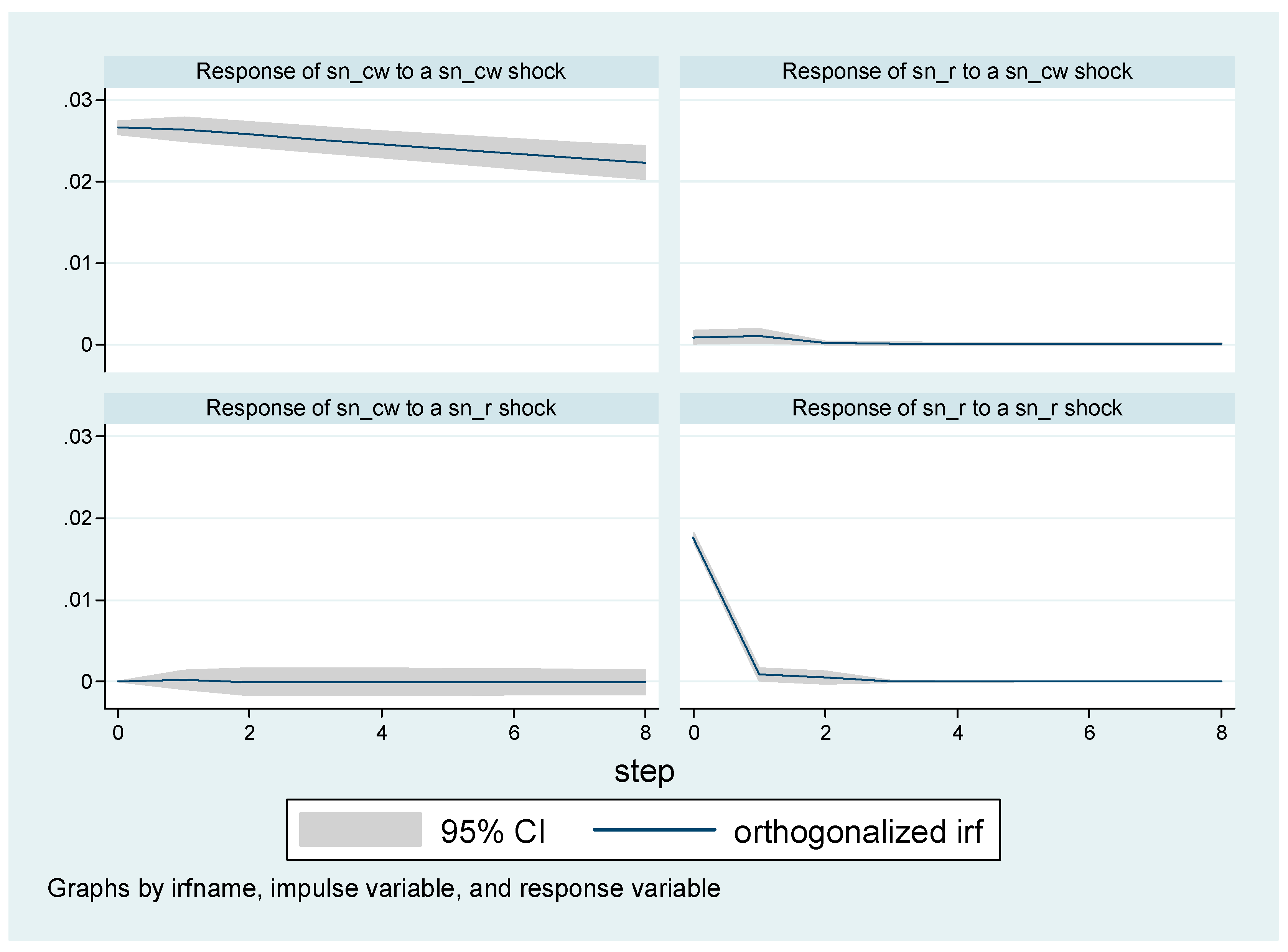
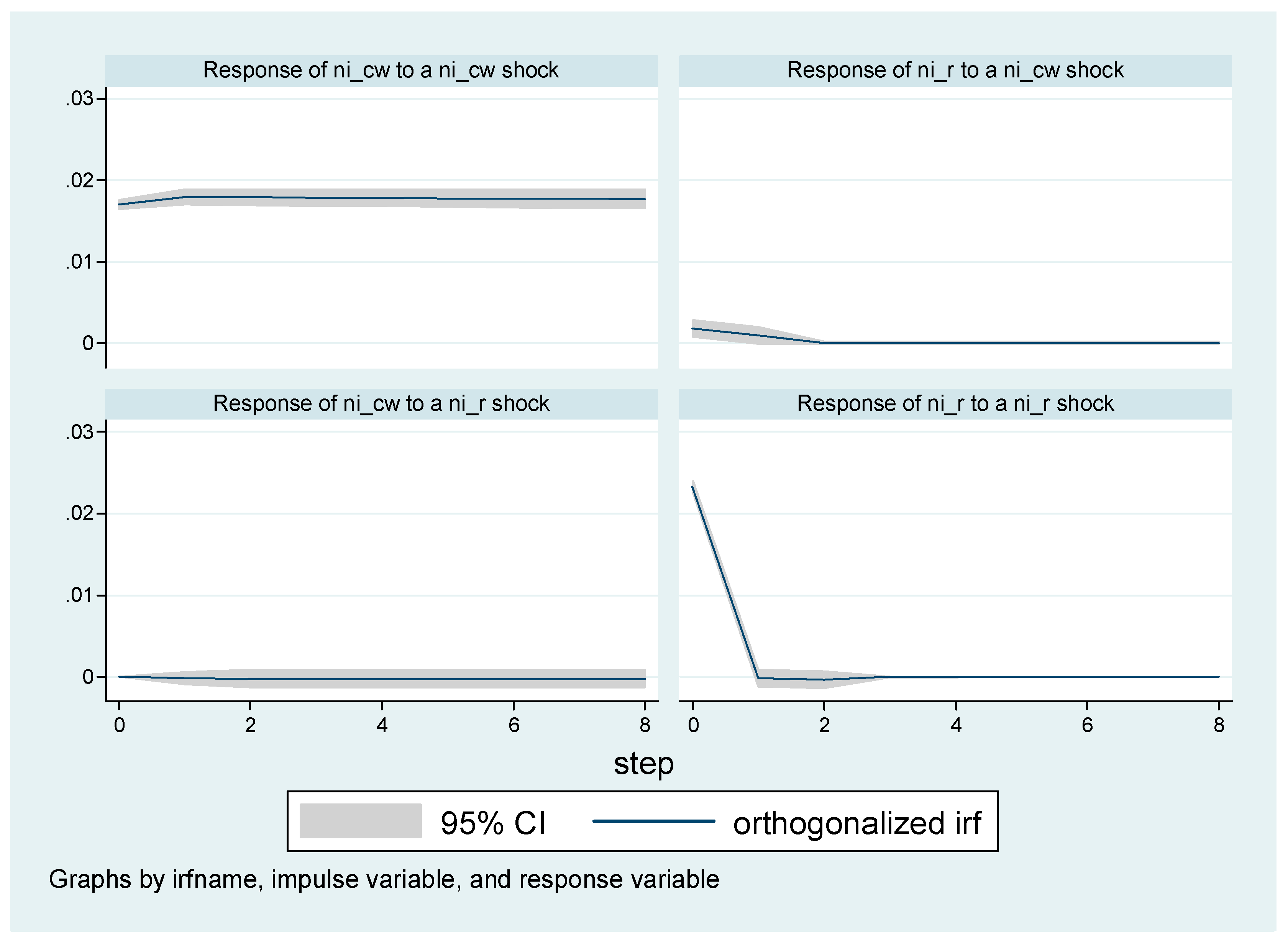
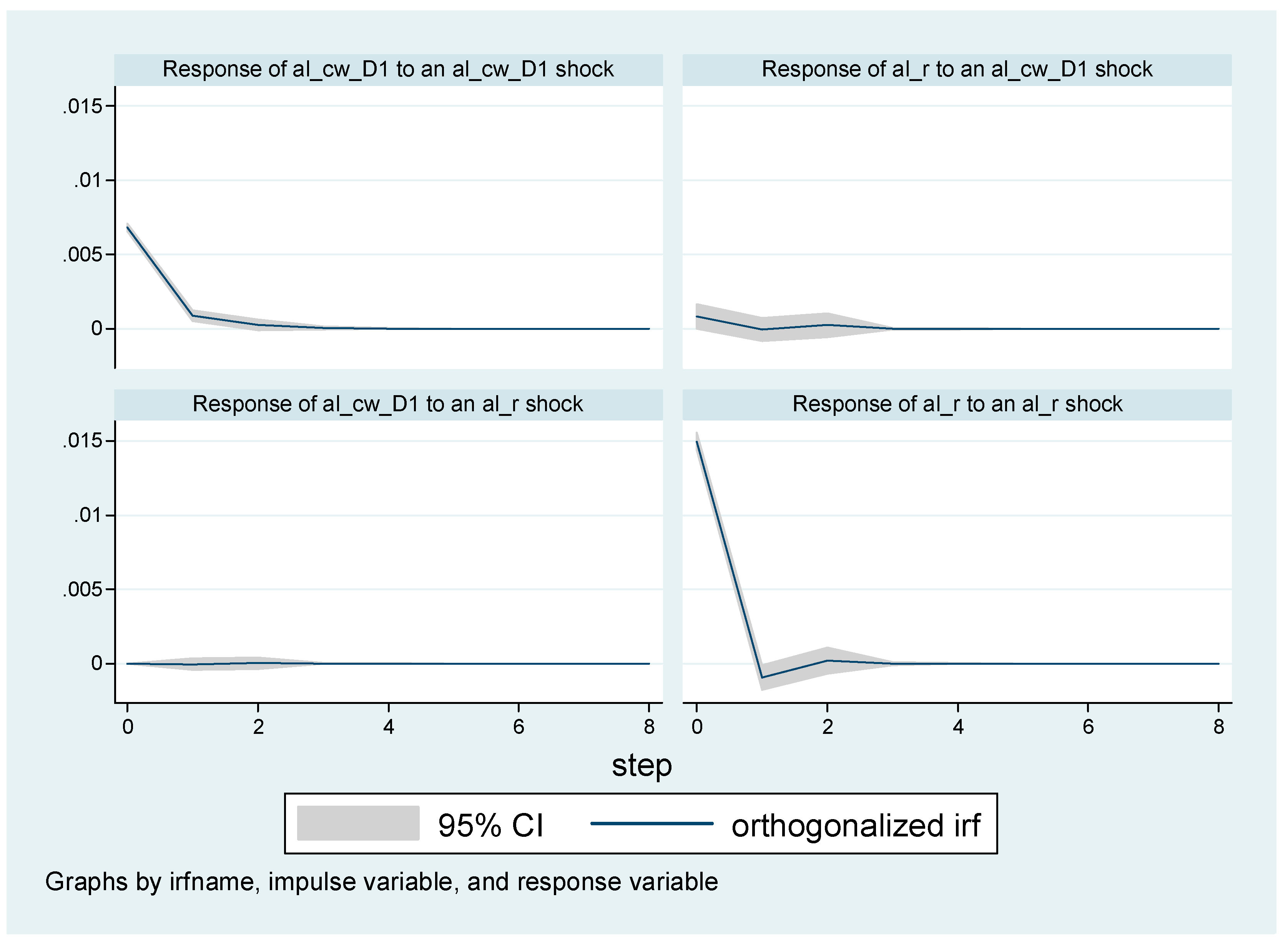
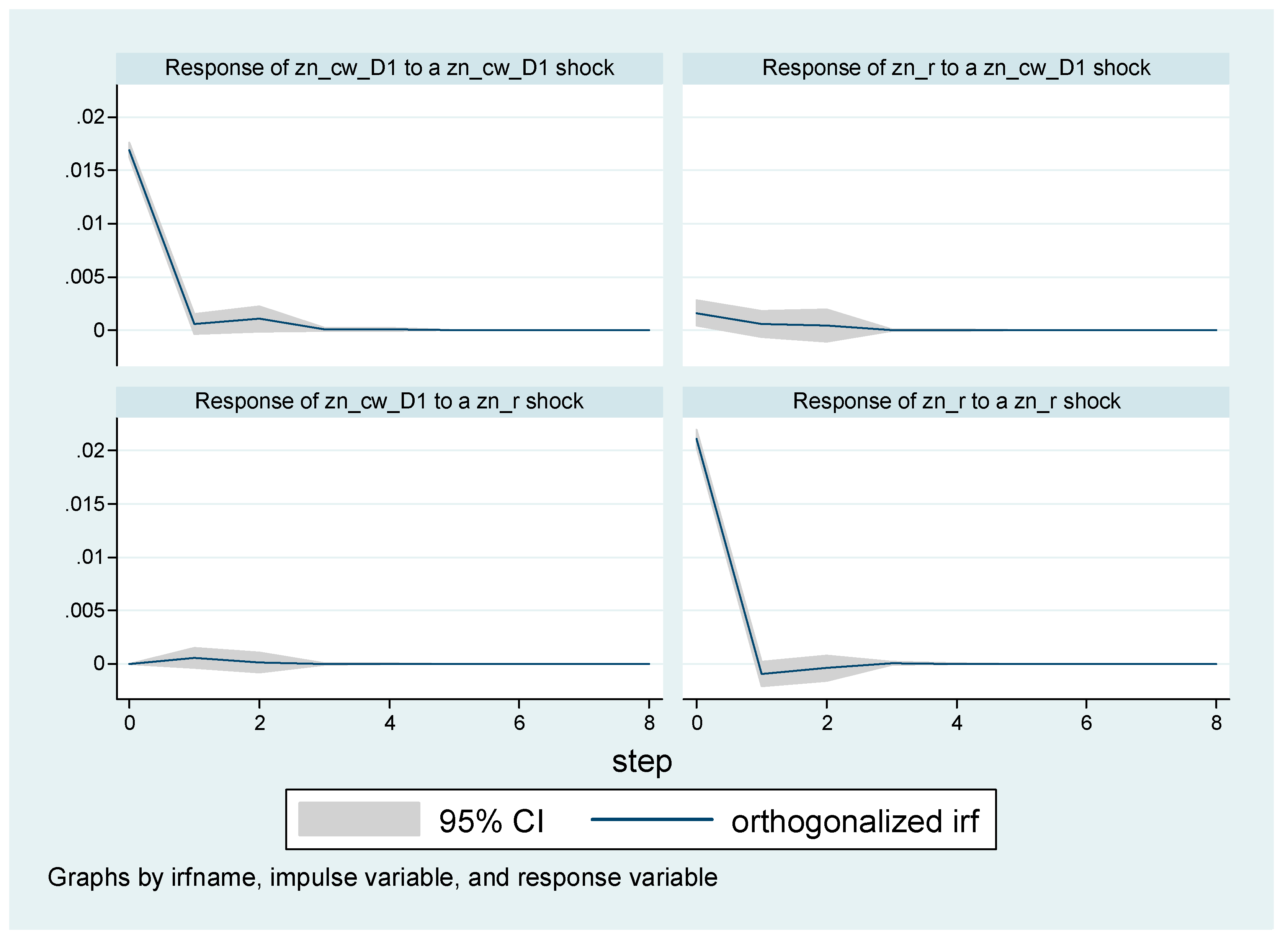
The VAR shown in Equation (2) is then estimated using the Stata 12 software. The results for the parameters, as well as some statistics, are not reported in this paper, but we do present the impulse response results. The impulse responses to spot returns to CW shock are shown in Figure 1. It is found that the impact of a CW shock on spot returns of both tin and nickel has second period positive effects. The positive effect on metal returns holds for the contemporaneous and first two lags following an increase in CWs, and then the positive effect on spot returns of a CW shocks fades after the second period. In Figure 2 there are the impulse responses to spot price returns of aluminum and zinc to CW shocks, which implies one more period impact compared to tin and nickel. In conclusion, the positive impact of the CWs to metal returns is transitory.

Guzman and Silva (2018) found similar result for the copper market using error variance decomposition. They reported that more than 19% of variance was associated with financial speculation, such as the long positions in the futures market during the period over August 2003 and September 2008. However, different periods, such as April 1995–March 2003 and October 2003–October 2015, showed a somewhat lowered effect.

5. Summary and Conclusions

Particular interest has been growing recently in the potential role of the financialization of commodity markets. This study establishes a hypothesis concerning whether the rise in CWs is associated with LME metal price increases. The CWs variable is important, because it encompasses two factors—fundamentals and non-fundamentals. It is a fundamentals variable because it relates to the market inventory. It is also a non-fundamentals variable because it deals with global sell-side brokers’ reports and affects investors’ sentiments. Using 13 years of daily data, first, this paper observes that there is a statistically significant positive link between CWs and LME metal prices, especially aluminum, zinc, tin, and nickel. I conclude that CWs intensify the aluminum, zinc, tin, and nickel spot prices direction. Second, the impulse response to a CW shock shows that the positive impact of the metal returns for aluminum, zinc, tin, and nickel is transitory rather than permanent, so that the effect of a unit shock in CWs eventually converges to zero. Indeed, after the second period, the positive effect on spot returns of a CW innovation dies out.

The link between CWs and spot prices has important implications for the pricing of the LME market, and ex post analysis of the reasons behind LME base metal prices. In the light of these results, it would be useful to test the effect of CW changes within various LME warehouses, such as Rotterdam, Vlissingen, New Orleans, Johor, and Busan, even though collecting data is somewhat difficult.

References

- Arouri, Mohamed El Hedi, Fredj Jawadi, and Prosper Mouak. 2011. The Speculative Efficiency of the Aluminum Market: A Nonlinear Investigation. International Economics 126–27: 73–89. [Google Scholar] [CrossRef]
- Canarella, Giorgio, and Stephen K. Pollard. 1986. The “Efficiency” of the London Metal Exchange: A Test with Overlapping and Non-Overlapping Data. Journal of Banking and Finance 10: 575–93. [Google Scholar] [CrossRef]
- Cheng, Ing-Haw, and Wei Xiong. 2014. Financialization of Commodity Markets. Annual Review of Financial Economics 6: 419–41. [Google Scholar] [CrossRef]
- Figuerola-Ferretti, Isabel, and Christopher L. Gilbert. 2008. Commonality in the LME Aluminum and Copper Volatility Processes through a FIGARCH Lens. The Journal of Futures Markets 28: 935–62. [Google Scholar] [CrossRef]
- Guzmán, Juan Ignacio, and Enrique Silva. 2018. Copper Price Determination: Fundamentals versus Non-fundamentals. Mineral Economics 31: 283–300. [Google Scholar] [CrossRef]
- Irwin, Scott H., and Dwight R. Sanders. 2012. Testing the Masters Hypothesis in commodity futures markets. Energy Economics 34: 256–69. [Google Scholar] [CrossRef]
- Kang, Sang Hoon, and Seong-Min Yoon. 2016. Dynamic Spillovers between Shanghai and London Nonferrous Metal Futures Markets. Finance Research Letters 19: 181–88. [Google Scholar] [CrossRef]
- Koitsiwe, Kegomoditswe, and Tsuyoshi Adachi. 2018. The Role of Financial Speculation in Copper Prices. Applied Economics and Finance 5: 87–94. [Google Scholar] [CrossRef]
- MacDonald, Ronald, and Mark Taylor. 1988. Metal Prices, Efficiency and Cointegration: Some Evidence from the LME. Bulletin of Economic Research 40: 235–39. [Google Scholar] [CrossRef]
- Otani, Kiyoshi. 1983. The Price Determination in the Inventory Stock Market: A Disequilibrium Analysis. International Economic Review 24: 709–19. [Google Scholar] [CrossRef]
- Otto, Sascha Werner. 2011. A Speculative Efficiency Analysis of the London Metal Exchange in a Multi-Contract Framework. International Journal of Economics and Finance 3: 3–16. [Google Scholar] [CrossRef]
- Park, Jaehwan. 2018. Volatility Transmission between Oil and LME Futures. Applied Economics and Finance 5: 65–72. [Google Scholar] [CrossRef]
- Park, Jaehwan. 2019. Effect of Speculators’ Position Changes in the LME Futures Market. Working Paper. under review. [Google Scholar]
- Park, Jaehwan, and Byungkwon Lim. 2018. Testing Efficiency of the London Metal Exchange: New Evidence. International Journal of Financial Studies 6: 32. [Google Scholar] [CrossRef]
- Singleton, Kenneth J. 2014. Investor Flows and the 2008 Boom/Bust in Oil Prices. Management Science 60: 300–18. [Google Scholar] [CrossRef]
- Tang, Ke, and Wei Xiong. 2012. Index Investment and the Financialization of Commodities. Financial Analysts Journal 68: 54–74. [Google Scholar] [CrossRef]