Article

The Impact of Government Expenditure in Agriculture and Other Selected Variables on the Value of Agricultural Production in South Africa (1983–2019): Vector Autoregressive Approach

Department of Agricultural Economics, University of Limpopo, Polokwane 0727, South Africa
*
Author to whom correspondence should be addressed.
Economies 2022, 10(9), 205; https://doi.org/10.3390/economies10090205
Submission received: 28 June 2022 / Revised: 28 July 2022 / Accepted: 29 July 2022 / Published: 24 August 2022

Abstract

:
South African agriculture has the potential to stimulate growth in other economic sectors, but dwindling budgetary allocations to agriculture over time and the nature of other impacting factors on the value of agricultural production have not received much attention in recent times. Therefore, the present study examined the effects of government expenditure in agriculture, annual average rainfall, consumer price index, food import value, and population on the value of agricultural production with a specific focus on government expenditure in agriculture for the period 1983 to 2019. Using the Johansen cointegration test, the results reveal that there is a long-run relationship among the variables. The Granger causality test results suggest that government expenditure in agriculture does not Granger cause the value of agricultural production. However, the two variables are linked through other variables in the model, such that an increase in government expenditure in agriculture, average annual rainfall, and population were shown to ultimately increase the value of agricultural production based on vector autoregressive (VAR) model analysis. In contrast, an increase in the consumer price index and food import value is detrimental to the value of agricultural production. These studies’ findings have policy implications for increased government expenditure.

1. Introduction

The value of agricultural production is crucial in determining the state of the agricultural sector when compared to other economic sectors (FAO 2017). According to the Food and Agricultural Organisation (FAO 2021), the value of agricultural production expresses total agricultural output in monetary terms, whereas in the South African context, the value of agricultural production is defined by the total production of field crops, horticultural crops, and livestock products valued at average farm-gate prices (DAFF 2019). Such value was recorded in 2019 at approximately US$46 million, US$62 million, and US$107 million for field crops, horticultural crops, and livestock products, respectively (DALRRD 2020). The contribution of agriculture to the gross domestic product (GDP) of South Africa is reported by Statistics South Africa (STATS SA 2020) to have expanded from 2.2% in 2010 to 2.3% in 2020, which remains low, yet agriculture is expected to boost employment in South Africa as noted in Allen et al. (2021). The Organisation of Economic Cooperation and Development (OECD 2020) reported that the value of agricultural production in South Africa is constantly fluctuating and manifests in the agricultural sector’s poor performance (Karfakis et al. 2011) among other sectors. Thus, unfolding the influential variables to the value of agricultural production is imperative.
A fluctuating value of agricultural production is observed when prices of agricultural products instantly become relatively high and low, and this affects both consumers and producers. To explain some of these fluctuations, the literature, such as Vasić et al. (2019), generally highlights the conflicting objectives of consumers aiming to purchase products at lower prices and producers aiming to sell their products at higher prices for profit maximization to the extent that an instant high value of agricultural production is advantageous for producers and detrimental for consumers. In interpreting such fluctuations, Nwer et al. (2021) alleged that there are factors that influence production in the agricultural sector, and Edeh et al. (2020) further noted that government expenditure is a tool mainly used to enhance economic growth through sectors, such as agriculture in Nigeria. Nevertheless, Iganiga and Unemhilin (2011) identified education, infrastructure, inflation, rainfall, and industrialization as factors that affect the value of agricultural production in Nigeria. It is acknowledged that the expenditure by the government in agriculture is ranked among the main sources of investment in agriculture (FAO 2022). However, government expenditure may be unproductive and consequently reduce the production value of sectors, such as agriculture (Moreno-Dodson 2008), whereby the availability of too much government expenditure can reduce private investments. According to Meniago et al. (2013), developing countries, such as South Africa, mainly depend on foreign direct investments for economic growth. Even though government expenditure is generally accepted as a driver of economic growth through sectoral development, Mo (2007) highlighted that government expenditure is not responsible for economic growth. Such discoveries establish the need to explore theories of government expenditure (discussed in Section 2.1) to understand advanced views on the relationship between government expenditure and growth-related variables, such as economic growth.
Aguera et al. (2020) report a poor government expenditure allocation in agriculture. The examination of the effect that government expenditure has on public sectors, such as agriculture has been overlooked in various studies (Chipaumire et al. 2014; Molefe and Choga 2017; Odhiambo 2015) that have analyzed the effect of government expenditure on the overall economy of South Africa and despite this, empirical studies on factors that affect the value of agricultural production are very few in South Africa. The present study differs from previous studies since it analyzes the effect of government expenditure on the sectoral level (agricultural sector) rather than the whole economy. In addition, the present study is different from most of the literature in South Africa because it analyzes the effect of selected variables on the value of agricultural output rather than on agricultural production output and agricultural productivity. The importance of this present study is derived from the need to analyze the effect of selected variables on the value of agricultural production with more interest in government expenditure on agriculture to further understand the main problem of a fluctuating value of agricultural production. Although this study was conducted in South Africa, global agriculture is diverse, fast-growing, and intertwined through trade (FAO 2018). This study is of global interest in the literature reporting that South Africa is developing similarly to other countries (aiming at improving agriculture). Thus, many countries have a common interest in research related to agricultural development. In addition, this present study explores the theme of government expenditure, which is an instrument for agricultural transformation in many countries (Goyal and Nash 2016), thus attracting international interest and readership.
Examining spending goals for the agricultural sector amid the consensus that the South African agricultural sector is known for job creation (Allen et al. 2021), a lot more must be understood in the context of government expenditure in the agricultural sector and agricultural production output. Matchaya (2020) highlighted that understanding the relationship between the value of agricultural production and government expenditure in agriculture helps in determining appropriate policy responses, which ultimately guarantee economic growth. Therefore, it is necessary to analyze the effect of government expenditure in agriculture on the value of agricultural production in South Africa, given that the literature is limited for the period evaluated in this study and that the findings could highlight possible policy implications particularly relevant in the context of the growth of the agricultural sector.
The agricultural sector is generally identified as the driver of economic growth in most developing countries (Mukasa et al. 2017; Pawlak and Kołodziejczak 2020; Bjornlund et al. 2020). Thus, the agricultural sector is subjected to size and structural changes to meet the changing economic environment over time (Greyling 2012). The changes in the size and structure of the South African agricultural sector and agricultural production can be traced back to the start of the 20th century (Liebenberg et al. 2011). The agricultural sector in South Africa has been playing a crucial role in economic growth through its production potential over the years. According to Pfunzo (2017), enhancing agricultural production positively influences economic growth. Hence, it is rational for governments to promote agricultural development amid all economic obstacles. This theoretical basis is further developed under the literature review.
The rest of the paper is organized as follows: Section 2 gives a literature review, followed by the methodology and presentation of findings in Section 3 and Section 4, respectively. The discussion is presented in Section 5. The conclusion is presented in Section 6. Section 7 focuses on future research.

2. Literature

This section is divided into two subsections, in which Section 2.1 presents the literature based on theories of government expenditure, such as Wagner’s theory and the Keynesian theory. Section 2.2 reviews the literature based on previous studies that are related to the present study.

2.1. Theoretical Literature

Based on the evidence of Wagner (1876), public expenditure is an endogenous variable that is used to stimulate the economy rather than as a cause of growth. In addition, Wagner (1876) proposed that in the process of economic development, the rate of public expenditure increases higher than the rate of economic growth and the causal relationship between public expenditure and economic growth and runs from economic growth to public expenditure and not vice versa as stated by the Keynesian theory. Considering this evidence, and with an appreciation that the growth of an economy, is an aggregate of sectoral growth; this present paper in agreement with (Lencucha et al. 2020), which posits that expanding the agricultural sector and its contribution to economic growth requires adequate measures, such as government expenditure, provided through the fiscal policy. Increasing government expenditure on important economic sectors, such as agriculture, ultimately enhances the economic activity and increases job creation (Ernawati et al. 2021). The need for increased government expenditure can be derived from the consensus that government expenditure is significant in promoting economic growth according to the Keynesian school of thought (Dynan and Sheiner 2018).
The Keynesian theory supports the idea that government expenditure is responsible for increasing domestic economic activity (Babatunde 2018). In addition, government expenditure is regarded as the main driver of economic growth (Keynes 1936), which is used to solve economic stagnation-related issues. In contrast to Wagner’s theory, the Keynesian theory considers government expenditure as an exogenous tool that governments use to always control economic growth (Selvanathan et al. 2021). Although Moreno-Dodson (2008) asserts that government expenditure may be unproductive, Keynes (1936) emphasizes that if governments stimulate government expenditure through fiscal policy, then business activities will increase within an economy. Practically, the Maputo declaration on spending on African agriculture is also premised upon the idea of adequate spending by governments suggesting that up to a 10% portion of countries’ overall budgets be allocated to agriculture (Sers and Mughal 2019). Additionally, Makin (2015) supports Keynes’s theory by attesting that increasing government expenditure leads to a higher national output value, which this present paper investigates sectorally by testing the relationship between government expenditure and the value of agricultural output. Government expenditure in agriculture is the total expenses incurred by the government on the agricultural sector (Atayi et al. 2020), covering expenses such as agricultural research, technology development, livestock, crop gene banks, and extension service (Mogues and Anson 2018).
The relationship between government expenditure in agriculture and the value of agricultural production is therefore examined herein in a six-variable autoregressive model described in Section 3. Previous research is discussed in the following subsection.

2.2. Previous Studies

Previous studies have employed various methods, such as the vector error correction model (VECM), multiple regression and correlation analysis, Cobb–Douglas production function, and autoregressive-distributed lag model (ARDL) to analyze the variables of interest in this present study.
Setshedi and Mosikari (2019) studied macroeconomic variables’ effects on South Africa’s agricultural productivity. They used the vector error correction model (VECM) to analyze time-series data for the period 1975 to 2016. Findings showed that increasing government expenditure on agriculture could increase agricultural productivity. In addition, the findings showed that an increase in the consumer price index reduces agricultural productivity. The study focused on agricultural productivity, which differs from this present study’s focus on the value of agricultural production (the total quantity produced expressed in monetary terms). Igwe and Esonwune (2011) conducted a study to determine the determinants of agricultural production, focusing more on government expenditure in Nigeria. They used publicly available time-series data for the period 1994 to 2007, which was analyzed using the multiple regression analysis and correlation analysis. The study’s findings suggested that the effect of government expenditure on agriculture is yet to improve agricultural production. Nevertheless, the study’s findings revealed that the total population, annual rainfall, and the total area cropped are significant determinants of agricultural production.
Enu and Attah-Obeng (2013) conducted a study with the aim to identify macroeconomic factors that influence agricultural production in Ghana. The study used the Cobb–Douglas production for analyzing data. The study’s findings confirmed that major macroeconomic factors that influence agricultural production are real GDP per capita, real exchange rate, and labor force. Furthermore, the findings suggested that an increase in the labor force increases agricultural production. Kadir and Tunggal (2015) examined the impact of macroeconomic factors on agricultural productivity in Malaysia using time-series data for the period 1980 to 2014. They used the autoregressive-distributed lag model (ARDL) to analyze the data. The study’s findings revealed that an increase in government expenditure, exports, and money supply leads to improved agricultural productivity while the exchange rate and inflation reduce agricultural productivity.
The VAR model and impulse response functions employed in this present study have also been used in various research (Endaylalu 2019; Olubokun et al. 2016) to analyze government expenditure and growth variables. The findings of Endaylalu (2019) revealed that government expenditure in Ethiopia is significant in promoting economic growth. However, the findings of Olubokun et al. (2016) showed that government expenditure transmits positive shocks to economic growth in the short-run and negative shocks in the long-run in Nigeria.

3. Methodology

This study used publicly available time-series annual data for the period 1983 to 2019, a timeframe of 36 years was used due to data availability. The data was collected from four sources: the Food and Agricultural Organisation (FAO), South African Reserve Bank (SARB), the World Bank, and Quantec databases. The Food and Agricultural Organisation provided yearly population (PG) statistics in this study, while SARB gives yearly government expenditure (GEA) in million rands. Moreover, the World Bank provided annual average rainfall (AAR) data in millimeters and a yearly consumer price index (CPI). Finally, Quantec databases provided annual data on the value of agricultural production (VAP) and food import value (FIV), both in million rands. Econometric Views (EViews) 12 statistical tool was used to generate empirical results for this research.

3.1. Unit Root Testing

The augmented Dickey–Fuller (ADF) test was used to test for unit root existence as a mandatory step for time-series data. The study adopted the regression equation given by Dickey and Fuller (1979), which is expressed as follows:
Δ Y t = α + β t + ϑ Y t 1 + i 1 k λ Δ × Y t 1 + μ t
where ΔYt is the first difference of the series Y; μ t is a stochastic error term, in which ΔYt−1 = (Yt−1Yt−2), ΔYt−2 = (Yt−2Yt−3); α is a constant; t is the time; and β and ϑ are parameters.
Unit root testing aims to test for the stationarity of time-series data. Unit root testing is essential for time-series analysis since the results generated with nonstationary time-series data can only be used for that certain period and cannot be ultimately used for predicting future values.

3.2. Cointegration Test

The Johansen cointegration test was used to check the existence of long-run relationships among the variables. The study employed two likelihood ratio tests, namely the trace test and the maximum eigenvalue test. Johansen (1988) expressed equations for both tests as follows:
J t r a c e = T i = r + 1 n ln ( 1 λ i )
z J m a x = T   ln ( 1 λ r + 1 )
where T is the sample size, λ i is the ith largest canonical correlation, and r is the number of cointegrating vectors. The null hypothesis is that there is no cointegration among the variables, and the null hypothesis is rejected when either the trace statistic or maximum eigenvalue statistic is greater than the critical value.

3.3. Granger Causality Test

The study used the Granger causality test to test for causality between subsets of variables. The Granger causality test establishes the direction of causality among the variables that are included in a system and show the relevance of one variable in predicting future values of other variables (Rasheed and Tahir 2012). The general formula given by Granger (1969) is expressed as follows:
X i = j = 1 m a j X t j + j = 1 m b j Y t j + e i
Y i = j = 1 m c j X t j + j = 1 m b j Y t j + n i
where X i and Y i are variables included in the system. The implication of Equations (4) and (5) is that that X i is Granger-causing Y t when a j is not zero, and Y t Granger cause X i when c j is not zero.

3.4. Model Specification

Vector autoregressive model provided a consistent and credible approach to data description, structural inference, forecasting, and policy analysis (Endaylalu 2019). The model is typically used in forecasting interconnected time-series systems establishing multiple equations (Gou 2017). For the interest of this study, a single equation was used where the value of agricultural production was treated as the dependent variable.
This research specified the single equation of the VAR model as follows:
V A P = F   ( G E A ,   C P I ,   A A R ,   F I V ,   P G )
where VAP = value of agricultural production, GEA = government expenditure in agriculture, AAR = average annual rainfall, CPI = consumer price index, FIV = food import value, and PG = population.
Introducing the logarithm on both sides of Equation (6), the stochastic model is expressed as follows:
l n V A P = β 0 + β 1   l n G E A + β 2   l n C P I + β 3   l n A A R + β 4   l n F I V + β 5   l n P G + μ
where lnVAP = log of value of agricultural production, lnGEA = log of government expenditure in agriculture, lnAAR = log of average annual rainfall, lnCPI = log of consumer price index, lnFIV = log of food import value, and lnPG = log of population.

3.5. Impulse Response Analysis and Variance Decomposition

This study used impulse response analysis to analyze the reaction of the value of agricultural production to the shocks of selected variables. The study also used the variance decomposition to determine how much each variable contributed to the value of agricultural production. Both tests considered a timeframe of ten years in forecasting.

4. Results

This section comprises four subsections in which Section 4.1 discusses empirical results of the augmented Dickey–Fuller test results (Table 1), vector autoregression lag order selection criteria (Table 2), Johansen cointegration test results (Table 3), Granger causality test results (Table 4), and the VAR model results (Table 5). Section 4.2 discusses the results of the model diagnostic tests, such as the residual portmanteau test for autocorrelations (Table 6), the inverse roots of the AR characteristic polynomial for stability (Figure 1), and heteroscedasticity test results (Table 7). Section 4.3 and 4.4 discuss impulse response analysis results and the decomposition of variation results, respectively.

4.1. Empirical Results

The results of the ADF unit root test presented in Table 1 indicate that all variables are stationary at levels and at first differences on all equations (either intercept, trend and intercept, or none) except the food import value (FIV), which is only stationary at first differences.
Table 1. Augmented Dickey–Fuller (ADF) Unit Root Test Results (In levels and 1st difference).
VariablesFormulaADF
Levels 5% Critical Value1st Difference5% Critical Value
VAPIntercept −3.111 **−2.951−2.222−2.976
Trend and intercept −0.706−3.587−0.898−3.587
None3.760 **1.9513.169 **−1.593
GEAIntercept0.969−2.945−6.393 **2.948
Trend and intercept−1.434−3.540−6.881 **−3.544
none3.057 **−1.950−0.852−1.952
AARIntercept−5.507 **−2.945−4.554 **−2.957
Trend and intercept −5.777 **−3.540−4.326 **−3.595
None −0.477−1.951−4.616 **−1.951
CPIIntercept 3.069 **−2.951−2.472−2.948
Trend and intercept−0.754−3.548−4.034 **−3.548
None−2.817 **−1.9511.080−1.952
FIVIntercept −1.749−2.971−1.271−2.957
Trend and intercept−2.427−3.580−5.892 **−3.548
None−1.575−1.952−0.474−1.951
PGIntercept −1.030−2.957−3.277 **−2.967
Trend and intercept−6.878 **−3.552−2.651−3.557
None1.409−1.951−0.518−1.951
Notes: Reported values under levels and first difference are ADF t-statistics values; ** Statistically significant at 5% level.
The null hypothesis that there is unit root existence is rejected for all variables at first differences, and therefore, it is concluded that the variables are integrated in the order I(1). The VAR model used was in first differences after performing the automatic lag selection presented in Table 2, as well as the test results for cointegration in the long-run presented in Table 3.
Table 2. Vector autoregression lag order selection criteria.
LagLogLLRFPEAICSCHQ
0−2019.344NA7.38 × 1042115.7340116.0006115.8260
1−1794.744359.36061.59 × 1038104.9568106.8232105.6011
2−1739.83869.02402 *6.54 × 1037 *103.8765 *107.3427105.0730 *
Notes: * indicates lag order selected by the criterion, (each test at 5% level). LR: sequentially modified LR test statistic, FPE: Final prediction error, AIC: Akaike information criterion, SC: Schwarz information criterion, HQ: Hannan–Quinn information criterion.
The leg length was chosen based on four criteria: LR, FPE, AIC, and HQ. All four criteria suggested the lag length of two, which was used when generating results of the VAR model.
Table 3. Johansen cointegration test results.
Trace TestMaximum Eigenvalue Test
Hypothesised No. of CE(s)EigenvalueTrace Statistics0.05 Critical ValueMaximum Eigenvalue Statistics0.05 Critical Value
None *0938192.076 **95.75355.004 **40.077
At most 1 *0.70897.072 **69.81841.966 **33.876
At most 2 *0.55155.106 **47.85627.26827.584
Notes: The trace test indicates three cointegrating eqn(s) at the 0.05 level; the max-eigenvalue test indicates two cointegrating equation(s) at the 0.05 level; * Denotes rejection of the hypothesis at the 0.05 level; ** Denotes cointegrating equations.
The trace test results suggest three cointegrating equations, and the maximum eigenvalue test suggests two cointegrating equations at a 5% significance level. Therefore, these findings confirm that there is a long-run equilibrium relationship between the value of agricultural production, government expenditure in agriculture, consumer price index, average annual rainfall, food import value, and population in South Africa. These findings suggest that there is a period in which all selected variables adjust fully to the changing agricultural economy. These studies’ findings establish the necessity for policymakers to closely monitor all selected variables in order to recommend policy measures that ensure that the long-run equilibrium point is reached, ensuring a stable value of agricultural production.
The results in Table 4 indicate that government expenditure in agriculture does not Granger cause the value of agricultural production.
Table 4. Granger causality test results.
Null HypothesisObs.F-Stat. Prob. Decision
DGEA does not Granger cause DVAP
DVAP does not Granger cause DGEA
34 included0.24541
1.59284
0.7840
0.2206
Accept
Accept
DCPI does not Granger cause DVAP
DVAP does not Granger cause DCPI
34 included0.39003
2.08565
0.6805
0.1425
Accept
Accept
DAAR does not Granger cause DVAP
DVAP does not Granger cause DAAR
34 included0.42173
2.13975
0.6599
0.1359
Accept
Accept
DFIV does not Granger cause DVAP
DVAP does not Granger cause DFIV
34 included9.92527
1.46711
0.0005 **
0.2472
Reject
Accept
DPG does not Granger cause DVAP
DVAP does not Granger cause DPG
34 included0.54354
0.29980
0.5865
0.7432
Accept
Accept
Notes: Granger cause if p < 0.05; ** Statistically significant at 5% level.
The results are supported by Singh et al. (2021) in India noting that government expenditure does not Granger cause the value of agricultural production output due to poor allocation of expenditure within the agricultural sector. The results also show that the value of agricultural production does not Granger cause government expenditure on agriculture. This proves that Wagner’s theory (Wagner 1876) does not support the agricultural sector in South Africa. There is no causality from the value of agricultural production to government expenditure in agriculture, wherein the expectation agrees with Wagner’s theory for growth (in the value of agricultural production) to cause public expenditure (government expenditure in agriculture). The food import value was found to Granger cause the value of agricultural production at significance level of 5%. Therefore, food import value is significant in forecasting the future values of the value of agricultural production in South Africa.
The VAR model results presented in Table 5 indicate that there is a positive significant relationship between government expenditure in agriculture (lnGEA) and the value of agricultural production (lnVAP) in the current year, confirming that increasing government expenditure in agriculture promotes agricultural production growth. It is also evident that a 1% increase in government expenditure on agriculture increases the value of agricultural production by 16% in the current year based on the coefficient of lnGEA. However, government expenditure in agriculture affects the value of agricultural production negatively in the second year, entailing the problem of diminishing marginal productivity of government expenditure in the agricultural sector according to the International Monetary Fund (IMF 2022). This finding reveals the need for assessing the current fiscal and monetary policies of South Africa to ensure consistency in the effects of government expenditure in the agricultural sector.
Table 5. VAR model results.
RegressorsCoefficientStd. Errort-StatProb.
lnVAP(-1) 0.638779 0.211706 3.017297 0.0031 **
lnVAP(-2) −0.073059 0.167798 −0.435402 0.6640
lnGEA(-1) 0.161955 0.077764 2.082641 0.0392 **
lnGEA(-2) −0.033866 0.069297 −0.488704 0.6259
lnCPI(-1) −0.208038 0.617256 −0.337037 0.7366
lnCPI(-2) −0.564957 0.625236 −0.903591 0.3679
lnAAR(-1) 0.088903 0.066007 1.346888 0.1803
lnAAR(-2) 0.120143 0.073278 1.639548 0.1035
lnFIV(-1) 0.146890 0.070018 2.097902 0.0378 **
lnFIV(-2) −0.234572 0.076503 −3.066171 0.0026 **
lnPG(-1)4.397032 6.377028 0.689511 0.4917
lnPG(-2) 1.527991 5.951629 0.256735 0.7978
C−57.09542 17.90459 −3.188870 0.0018
Notes: ** Statistically significant at 5% level; Observations: 35; R-squared 0.997982; mean dependent var 11.02903; adjusted R-squared 0.996882; S.D. dependent var 1.005709; S.E. of regression 0.056160; sum squared residuals. 0.069386; Durbin–Watson stat 2.418308.
There is a positive relationship between average annual rainfall (lnAAR) and the value of agricultural production in the current year and in the second year, confirming that an increase in rainfall is essential in enhancing the value of agricultural production. This finding is expected and is consistent with the findings of Eticha et al. (2021), which reveal that rainfall increases agricultural production. Furthermore, a 1% increase in annual average rainfall increases the value of agricultural production by 8.89% and 12.01% in the current year and the second year, respectively, based on the coefficients of lnAAR.
The population (lnPG) has a positive relationship with the value of agricultural production in the current year and the second year. This finding shows that an increase in population increases the value of agricultural production. These results agree with the findings of Schneider et al. (2021), which confirm that population is a driver of agricultural production.
There is a significant positive relationship between food import value (lnFIV) and the value of agricultural production in the current year, confirming that an increase in food imports increases the value of agricultural production. These results are not consistent with the findings of Sun et al. (2018), which revealed that importing food is detrimental to the agricultural land and ultimately agricultural production of an importing country. Even though food imports are known for ensuring food availability in the importing country and allowing growth (Porkka et al. 2017), the present study found that, in the second year, food imports have a negative relationship with the value of agricultural production. A 1% increase in food import value reduces the value of agricultural production by 23.34% based on the coefficient of lnFIV. Iganiga and Unemhilin (2011) agree with the present study that food import value reduces the value of agricultural production, meaning that importing food from other countries results in a decline in local agricultural production.
The consumer price index (lnCPI) has a negative effect on the value of agricultural production in the current year and the second year showing that a 1% increase in the consumer price index reduces the value of agricultural production by 20.8% and 56.49% in the current year and second year, respectively, based on the coefficients of lnCPI. These results agree with other studies (Setshedi and Mosikari 2019; Gou 2017), which agree with the present study that the consumer price index negatively influences the value of agricultural production. These results suggest that the inflation should always be regulated efficiently to prevent the value of agricultural production from fluctuating.

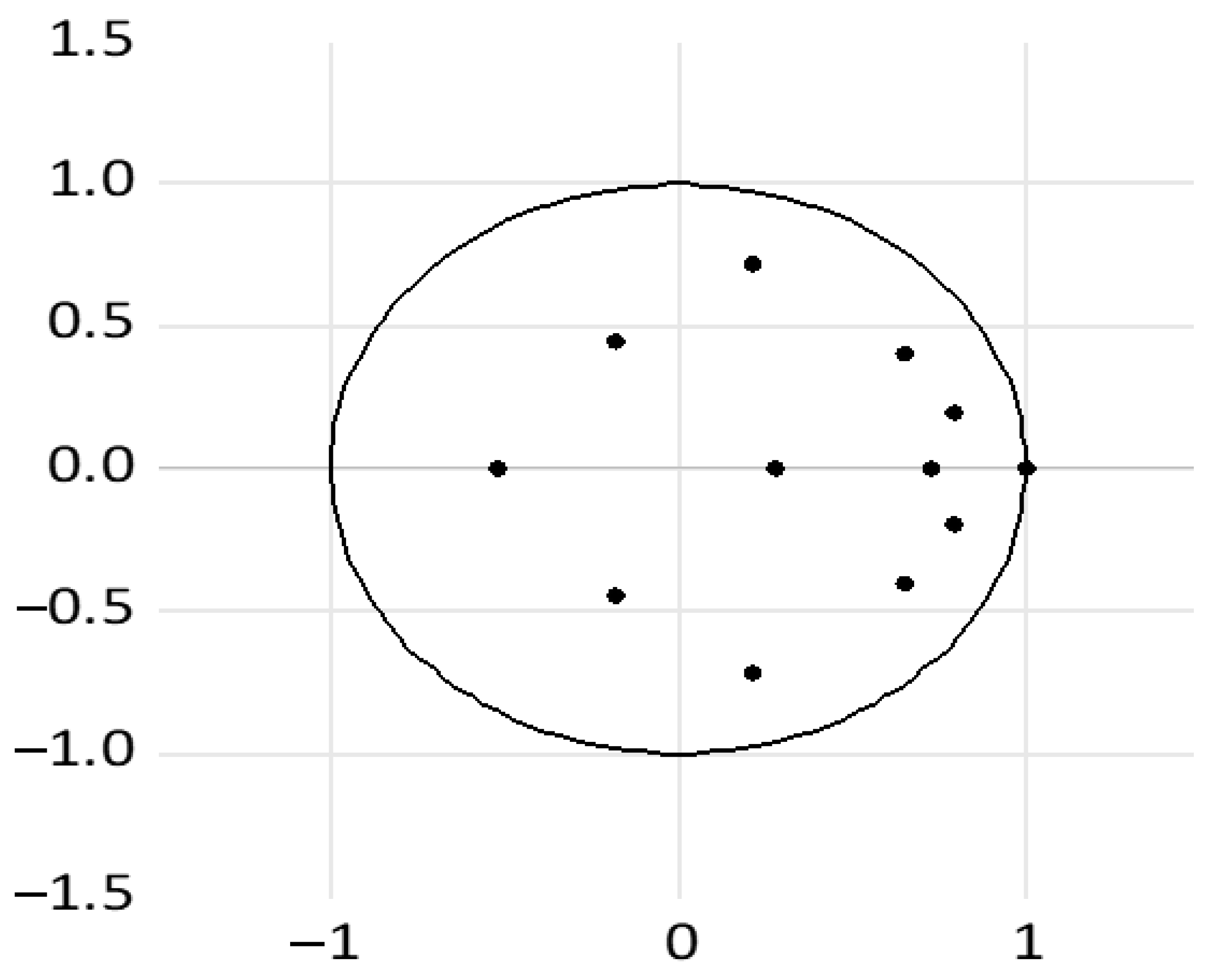
4.2. Model Diagnostic Check

A serial autocorrelation test was conducted using the residual portmanteau test.
As shown in Table 6, all probability values are greater than 0.05 level of significance. Therefore, we conclude that there is no autocorrelation problem in the estimated VAR model.
Table 6. Residual portmanteau test for autocorrelations.
LagsQ-StatProb.Adj. Q-StatProb
132.414220.639933.367580.5944
267.289690.635270.356720.5328
399.212000.7154105.27170.5564
4141.16340.5513152.63620.2952
5165.26290.7774180.75230.4702
6201.94470.7451225.02340.3227
7219.01350.9343246.35940.5884
8242.51610.9760276.82580.6714
9258.87410.9886312.30770.6696
10298.26030.9923353.44840.6874
11317.01950.9986380.80550.6996
12348.1986 0.9988 428.2483 0.5419
Figure 1 shows the inverse roots of the autoregressive (AR) characteristic polynomial, in which most inverse roots are within the borders of the circle and one on the circle line. These results imply that the vector autoregressive model is stable.
Figure 1. Inverse roots of the AR characteristic polynomial.
Economies 10 00205 g001
Table 7 shows the heteroscedasticity test results, in which the null hypothesis is that there is no heteroscedasticity problem. The probability value is greater than 0.05. Therefore, the null hypothesis that there is no heteroscedasticity problem in the estimates is accepted.
Table 7. Heteroscedasticity test.
TestH0dfT-StatisticProb. Conclusion
Chi-sq.No heteroscedasticity504525.13180.2491Accept H0, Prob. is greater than 0.05. Therefore, there is no heteroscedasticity
Accept H0: if Prob. > 0.05.

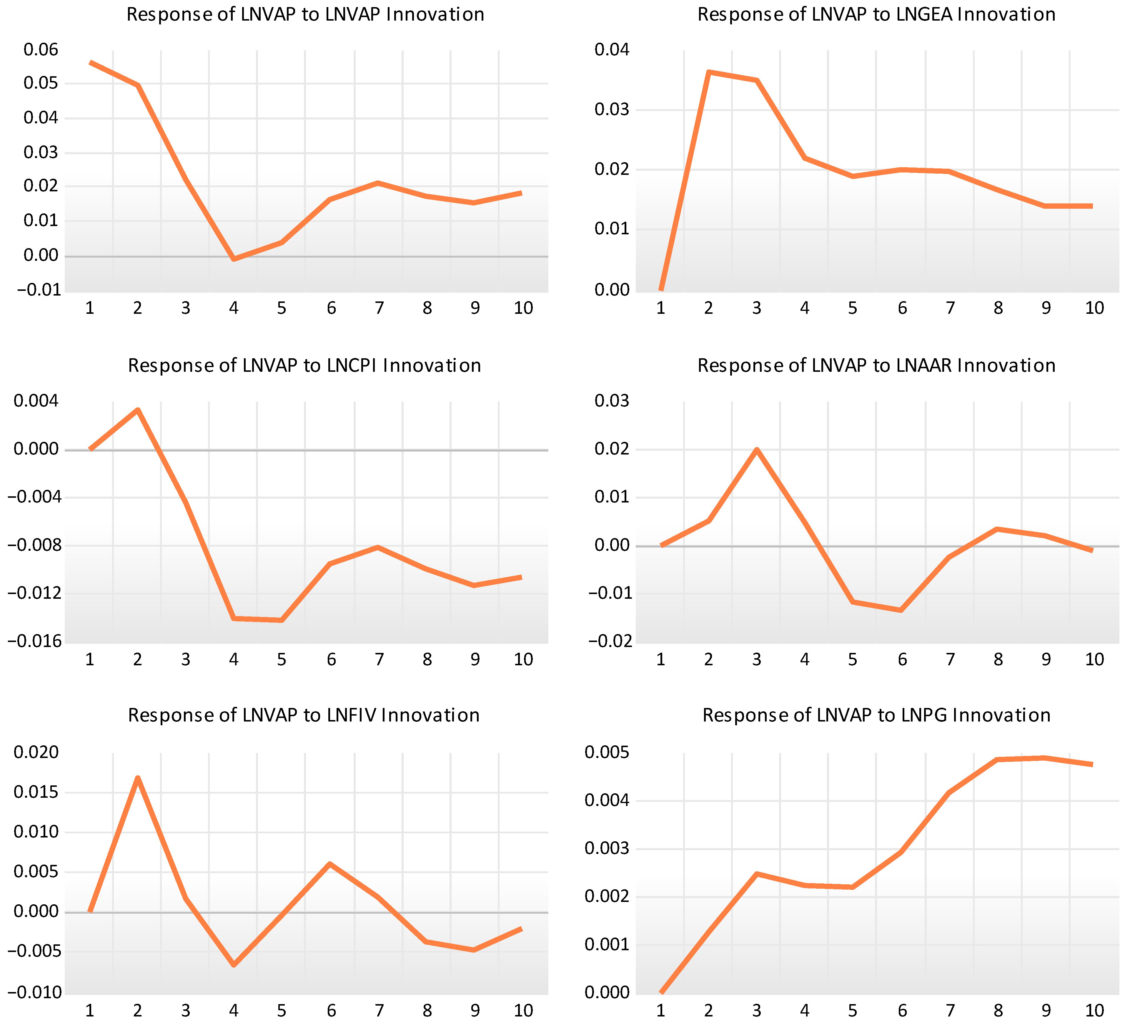
4.3. Impulse Response Analysis

Figure 2 represents the impulse responses of the value of agricultural production to the shocks of itself and all other selected variables used in the present study for ten years. The positive effect is indicated when the line is above (0.0), and the negative effect is shown when the line is below (0.0).
The results show that the value of agricultural production, government expenditure in agriculture, and population transmit positive shocks to the value of agricultural production for ten years. The slope of government expenditure shocks is positive in the short-run and negative in the long-run. This implies that additional units of government expenditure in agriculture reduce the value of agricultural production in the long-run, which is in line with the results of the VAR model. In addition, this can be caused by poor management and allocation of government expenditure in the agricultural sector as stated in the Granger causality test results in Section 4.1. Although government expenditure is generally known to be significant in improving sectoral productivity, there should be adjustments in policies, such as the fiscal policy, which regulates government expenditure to prevent unproductive government expenditure as stipulated by Moreno-Dodson (2008).
The consumer price index and food import value transmit positive shocks to the value of agricultural production in the short-run and adverse shocks in the long-run. These results agree with what the study recorded in the VAR model results. These results imply that the consumer price index and food import value are detrimental to the value of agricultural production when they increase. For the South African value of agricultural production to be stable, measures to lower the consumer price index and reduce food imports should be prioritized in policy making.

4.4. Variance Decomposition Analysis

Table 8 shows the results of the decomposition variation. The results indicate that shocks in the value of agricultural production (lnVAP) were the main drivers of VAP in South Africa as compared to other selected variables. Therefore, these findings mean that the South African value of agricultural production in the context of the VAR system used in the study can be predicted by its previous behavior. After the first year, the primary influence on South Africa’s value of agricultural production was government expenditure in agriculture shocks (lnGEA, accounting for 18.11%), followed by food import value (lnFIV, accounting for 3.93%), consumer price index (lnCPI, accounting for 0.13%), and average annual rainfall (lnAAR, accounting for 0.34%). The magnitude of population contribution to VAP did not change significantly between the second year and the tenth year because the annual population growth of South Africa in the study period (1983 to 2019) ranged between 1.33% and 2.8%, according to the United Nations (UN 2022), which is not drastically high.

5. Discussion

This section provides an in-depth interpretation as well as the implications of the results of the Granger causality test and the VAR model presented in Table 4 and Table 5 respectively.

5.1. Granger Causality Results in Discussion

The Granger causality results contribute to the literature by establishing that some included economic variables are useful in predicting future values of other economic variables in the system; it was found that government expenditure in agriculture is not useful in predicting future values of agricultural production value. The possible reason why government expenditure in agriculture is not useful in predicting the future value of agricultural production in South Africa is the consensus that government expenditure is still poorly allocated in the agricultural sector (Aguera et al. 2020), considering that poor resource allocation leads to poor increases in sectoral production (Nguyen and Luong 2021). These results imply that government expenditure in agriculture alone cannot be used to predict future values of the value of agricultural production. However, this does not imply that there is no relationship between government expenditure on agriculture and the value of agricultural production (the relationship is further discussed in Section 5.2). These results establish a need to properly and efficiently allocate government expenditure in agriculture to ultimately boost agricultural production. Contrary to the findings on government expenditure in agriculture not being useful in predicting the future value of agricultural production, food import value was confirmed to be useful. This finding is expected and consistent with the NAMC (2021) observation, highlighting that most unprocessed agricultural products imported by South Africa are due to the limited production capacity and unfavorable planting conditions even though food is sufficient (DAFF 2018). These results mean that food import value is a variable that can accurately predict how agricultural production value will behave in the future. These two variables are theoretically linked through prices of domestic and import products, however a further examination of those aspects is beyond the scope of this study.

5.2. VAR Findings Discussion

The results of the VAR single equation contribute to the literature by adding knowledge to the limited body of knowledge regarding the value of agricultural production. Government expenditure on agriculture were found to significantly improve agricultural production value (Table 5), though there is no causation established (Table 4). These results suggest that governments can use public spending for the agricultural sector to augment performance in agricultural production. These findings are generally expected and supported by various studies (Setshedi and Mosikari 2019; Keynes 1936; Iganiga and Unemhilin 2011), which confirm the relevance of government expenditure in ensuring agricultural growth and other related growth variables. For the South African government, these findings imply that the fiscal policy should be adjusted so that more expenditure is allocated to the agricultural sector to promote agricultural development and, ultimately, stabilize the value of agricultural production. Increasing government expenditure on agriculture will curb the problem of poor allocation (suggested in Section 5.1), ensuring that government expenditure on agricultural production is useful in predicting the future behavior of the value of agricultural production.
Another expected finding is that high rainfall increases the value of agricultural production. Rainfall is generally associated with increased agricultural production output, and agricultural production output directly influences the value of agricultural production in terms of scale quantities. Therefore, rainfall is important since most horticultural crops, and field crops, which contribute significantly to the value of agricultural production (DAFF 2019), depend heavily on rainfall suggesting that South Africa and most developing countries practice rainfed agriculture. These results imply that governments must prioritize the use of climate change (which is of global concern) mitigation strategies, such as climate smart technologies, that will ultimately improve climate change adaptation response for improved agricultural production in the wake of climate impacts on rainfall intensity.
Although not a direct relationship, the findings imply that population plays a role in increasing the value of agricultural production. An increase in population ultimately can increases the labor force, which is essential in increasing agricultural production according to the findings of Enu and Attah-Obeng (2013). The labor force of South Africa is estimated to be 22.6 million and increasing exponentially according to the World Bank (2022). Moreover, an increase in population not only increases the labor force but also leads to excessive consumption (Ganivet 2019), which stimulates agricultural production due to the high demand for agricultural products. Therefore, when the population increases, the labor force and the demand for agricultural products also increase. Due to the increased scale of production, an increase in the value of agricultural production can be expected. The implication of these results might focus on job creation to ensure that an adequate labor force is employed wherein income earned can induce affordability of agricultural products at all times. This favors both consumers and producers in a manner that consumers maximize their utilities while producers maximize their profits (as stated in the introduction section).
Food import value was found to increase the value of agricultural production in the short-run and to be detrimental to the value of agricultural production in the long-run. South Africa is food sufficient and sufficient in terms of agricultural production (USDA 2022). Therefore, when a country that is self-sufficient in production imports food from other countries, local agricultural producers are negatively affected (Clapp 2017) in the long-run. Thus, tempering with the value of agricultural production since the value of agricultural production is derived from prices that are received by producers at farm-gate. These results imply that self-sufficient countries that have the same structural conditions as South Africa may need to consider import substitution as a way to promote local agricultural production of major imported products.
The consumer price index was confirmed to be unfavorable in terms of impacts on the value of agricultural production in a manner that an increase in the consumer price index decreases the value of agricultural production, possibly through indirect channels when consumers resist price increases and reduce their demand for agricultural output. These results are generally expected, and they suggest that inflation (measured in CPI) should always be regulated efficiently through the monetary policy by central banks, such as The South African Reserve Bank (SARB), to prevent the value of agricultural production from fluctuating.

6. Conclusions

This paper considers the value of agricultural production as a significant factor that can be used in determining the state of the agricultural sector. Therefore, this paper explores the effect of selected variables on the value of agricultural production, focusing more on government expenditure for the period 1983 to 2019.
Based on the results of this paper, priorities by the government of South Africa should be on increasing government expenditure in agriculture while considering allocating the expenditure adequately. Increasing government expenditure in agriculture will ensure that the sector produces sufficient research and enhances modern technologies for better production. The government can spend adequately by investing in climate-smart agriculture research to ensure that climate-friendly technologies are developed and adopted. The use of climate-friendly technologies will ultimately ensure that the country receives enough rainfall for agricultural purposes. There is also a need to review the monetary policy responsible for controlling inflation (measured in CPI) in South Africa. If the monetary policy was structured efficiently, then prices of agricultural commodities at farm-gate would be stable during all phases of economic activity. Meaning that the value of agricultural production would also be stable since it measures aggregated farm-gate prices of agricultural products.

7. Limitations and Suggestions for Future Research

This study might not have focused on all variables affecting agricultural production value due to the limited literature and data availability. Some of the literature on agricultural production output and agricultural productivity was referenced because the literature on the value of agricultural production is very limited; hence, this study contributes toward the research knowledge on the value of agricultural production. To add to the literature concerning the value of agricultural production, future research can investigate the effect of other variables, such as interest rates, policy reforms, land, temperature, the value of exports, and fuel prices. In addition, future research can focus on modelling technical and allocative efficiencies of government expenditure in agriculture.

Author Contributions

Conceptualization, E.N. and C.L.M.; methodology, E.N. and C.L.M.; software, E.N.; writing—original draft preparation, E.N. and C.L.M.; validation, E.N. and C.L.M.; writing—reviewing and editing, E.N. and C.L.M.; visualization, E.N. and C.L.M.; supervision, C.L.M.; funding acquisition, E.N. and C.L.M. All authors have read and agreed to the published version of the manuscript.

Funding

This research was funded by the National Research Foundation (NRF) of South Africa: Postgraduate Scholarship, grant number 140973 and the APC was funded by the University of Limpopo.

Institutional Review Board Statement

Not applicable.

Informed Consent Statement

Not applicable.

Data Availability Statement

This study used publicly available data from the Food and Agricultural Organisation (FAO), South African Reserve Bank (SARB), the World Bank, and Quantec databases.

Conflicts of Interest

The authors declare no conflict of interest.

References

  1. Aguera, Pablo, Berglund Nils, Chimembiri Tapiwa, Comninos Alex, Gillwald Alison, and Govan-Vassen Naila. 2020. Paving the Way Towards Digitalizing Agriculture in South Africa. Available online: https://researchictafrica.net/wp/wpcontent/uploads/2020/09/PavingthewaytowardsdigitalisingagricultureinSouthAfricaWhitepaper272020105251.pdf (accessed on 19 March 2022).
  2. Allen, Caitlin, Asmal Zaakhir, Bhorat Haroon, Hill Robert, Monnakgotla Jabulile, Oosthuizen Morné, and Rooney Chris. 2021. Employment Creation Potential, Labour Skills Requirements, and Skill Gaps for Young People: A South African Case Study. Development Policy Research Unit Working Paper No. 202102. Cape Town: University of Cape Town. Available online: http://www.dpru.uct.ac.za/Publications/Working_Papers/DPRU%20WP202102.pdf (accessed on 5 April 2022).
  3. Atayi, Abraham V., Boniface JirboVerr, Awopetu O. Bobola, and Adekunle S. Olorunrinu. 2020. The Effect of Government Expenditure on Agricultural Output in Nigeria (1981–2018). International Journal of Applied Management Science 3: 1–14. [Google Scholar]
  4. Babatunde, Shakirat A. 2018. Government Spending on Infrastructure and Economic Growth in Nigeria. Economic Research-Ekonomska Istraživanja 31: 997–1014. [Google Scholar] [CrossRef] [Green Version]
  5. Bjornlund, Vibeke, Bjornlund Henning, and Andre F. Van Rooyen. 2020. Why Agricultural Production in Sub-Saharan Africa Remains Low Compared to the Rest of the World-A Historical Perspective. International Journal of Water Resources Development 3: 20–53. [Google Scholar] [CrossRef]
  6. Chipaumire, Gabriel, Hlanganipai Ngirande, Mangena Method, and Ruswa Yewukai. 2014. The Impact of Government Spending on Economic Growth: Case South Africa. Mediterranean Journal of Social Sciences 5: 109–18. [Google Scholar] [CrossRef] [Green Version]
  7. Clapp, Jennifer. 2017. Food self-sufficiency: Making Sense of it, and when it Makes Sense. Food Policy 66: 88–96. [Google Scholar] [CrossRef] [Green Version]
  8. DAFF. 2018. Self-Sufficiency Index. Available online: https://www.dalrrd.gov.za/Portals/0/Statistics%20and%20Economic%20Analysis/Economic%20Analysis/SSI%20Report%20Mar%202018.pdf (accessed on 26 July 2022).
  9. DAFF. 2019. Trends in the Agricultural Sector 2019. Available online: https://www.dalrrd.gov.za/Portals/0/Statistics%20and%20Economic%20Analysis/Statistical%20Information/Trends%20in%20the%20Agricultural%20Sector%202019.pdf (accessed on 4 May 2021).
  10. DALRRD. 2020. Economic Review of the South African Agriculture. Available online: https://www.dalrrd.gov.za/Portals/0/Statistics%20and%20Economic%20Analysis/Statistical%20Information/Economic%20Review%202020.pdf (accessed on 23 March 2022).
  11. Dickey, Alan D., and Wayne A. Fuller. 1979. Distribution of the Estimators for Autoregressive Time Series with a Unit Root. Journal of the American Statistical Association 74: 427–31. [Google Scholar]
  12. Dynan, Karen, and Louise Sheiner. 2018. GDP as a Measure of Economic Well-Being. Hutchins Center Working Paper No. 43. Washington, DC: Bookings Institution. Available online: https://www.brookings.edu/wp-content/uploads/2018/08/WP43-8.23.18.pdf (accessed on 22 June 2022).
  13. Edeh, Chukwudi Emmanuel, Chidera G. Eze, and Sonia O. Ugwuanyi. 2020. Impact of Foreign Direct Investment on the Agricultural Sector in Nigeria (1981–2017). African Development Review 32: 551–64. [Google Scholar] [CrossRef]
  14. Endaylalu, Solomon. 2019. The Impact of Public Expenditure Components on Economic Growth in Ethiopia; Vector Autoregressive Approach. International Journal of Business and Economics Research 8: 211–19. [Google Scholar]
  15. Enu, Patrick, and Prudence Attah-Obeng. 2013. Which Macro Factors Influence Agricultural Production in Ghana? Academic Research International 4: 333–46. [Google Scholar]
  16. Ernawati, Ernawati, Tajuddin Tajuddin, and Syamsir Nur. 2021. Does Government Expenditure Affect Regional Inclusive Growth? An Experience of Implementing Village Fund Policy in Indonesia. Economies 9: 164. [Google Scholar] [CrossRef]
  17. Eticha, Tolera K., Abdi K. Rikiti, Soresa S. Abdisa, and Adugna G. Ejeta. 2021. Assessing Effects of Rainfall on Farming Activities as the Predictor of Climate Changes in Sadi Chanka District of Kellem Wolega, Oromia, Ethiopia. Journal of Water and Climate Change 12: 3297–307. [Google Scholar] [CrossRef]
  18. FAO. 2017. The Future of Food and Agriculture. Trends and Challenges. Available online: https://www.fao.org/3/i6583e/i6583e.pdf (accessed on 23 June 2022).
  19. FAO. 2018. The Future of Food and Agriculture Alternative Pathways to 2050. Available online: https://www.fao.org/3/I8429EN/i8429en.pdf (accessed on 28 July 2022).
  20. FAO. 2021. Statistic Documents. Available online: http://fenixservices.fao.org/faostat/static/documents/QV/QV_e.pdf (accessed on 3 May 2021).
  21. FAO. 2022. Government Expenditures in Agriculture 2001–2020. Global and Regional Trends. FAOSTAT Analytical Briefs Series No. 35. Available online: https://www.fao.org/3/cb8314en/cb8314en.pdf (accessed on 16 June 2022).
  22. Ganivet, Elias. 2019. Growth in Human Population and Consumption both need to be Addressed to Reach an Ecologically Sustainable Future. Environment, Development and Sustainability 22: 4979–98. [Google Scholar] [CrossRef]
  23. Gou, Guohua H. 2017. The Study on the Relationship between Agricultural Product Price Fluctuation and Inflation. Journal of Service Science and Management 10: 166–76. [Google Scholar] [CrossRef] [Green Version]
  24. Goyal, Aparajita, and John Nash. 2016. Reaping Richer Returns Public Spending Priorities for African Agriculture Productivity Growth. Available online: https://thedocs.worldbank.org/en/doc/988141495654746186-0010022017/original/E3AFRReapingRicherReturnsOverview.pdf (accessed on 28 July 2022).
  25. Granger, Clive W. J. 1969. Investigating Causal Relations by Econometric Models and Cross Spectral Methods. Journal of Econometrica 37: 424–38. [Google Scholar] [CrossRef]
  26. Greyling, Jan C. 2012. The Role of the Agricultural Sector in the South African Economy. Master’s Thesis, Stellenbousch University, Stellenbosch, South Africa. [Google Scholar]
  27. Iganiga, Benson O., and Davidson O. Unemhilin. 2011. The Impact of Federal Government Agricultural Expenditure on Agricultural Output in Nigeria. Journal of Economics 2: 81–88. [Google Scholar] [CrossRef]
  28. Igwe, Kelechi, and Cynthia Esonwune. 2011. Determinants of Agricultural Output: Implication on Government Funding of Agricultural Sector in Abia State, Nigeria. Journal of Economics and Sustainable Development 2: 86–90. [Google Scholar]
  29. IMF. 2022. Unproductive Public Expenditures: A Pragmatic Approach to Policy Analysis. Available online: https://www.imf.org/external/pubs/ft/pam/pam48/pam4801.htm (accessed on 9 June 2022).
  30. Johansen, Søren. 1988. Statistical Analysis of Cointegration Vectors. Journal of Economic Dynamics and Control 12: 231–254. [Google Scholar] [CrossRef]
  31. Kadir, Shariff U. S. A., and Noor Z. Tunggal. 2015. The Impact of Macroeconomic Variables on Agricultural Productivity in Malaysia. South-East Asia Journal of Contemporary Business, Economics and Law 8: 21–27. [Google Scholar]
  32. Karfakis, Panagiotis, Velazco Jackeline, Moreno Esteban, and Covarrubias Katia. 2011. Impact of Increasing Prices of Agricultural Commodities on Poverty. ESA Working Paper No. 11–14. Rome: Food and Agriculture Organization. Available online: https://www.fao.org/3/am320e/am320e.pdf (accessed on 25 January 2022).
  33. Keynes, John M. 1936. The General Theory of Employment, Interest, and Money. London: Macmillan, pp. 1–190. [Google Scholar]
  34. Lencucha, Raphael, Nicole E. Pal, Appau Andriana, Thow Anne-Marie, and Drope Jeffrey. 2020. Government Policy and Agricultural Production: A Scoping Review to Inform Research and Policy on Healthy Agricultural Commodities. Globalization and Health 16: 1–15. [Google Scholar] [CrossRef] [Green Version]
  35. Liebenberg, Frikkie, Philip G. Pardey, and Kahn Micheal. 2011. South African Agricultural R and D Investments: Sources, Structure, and Trends, 1910–2007. Agrekon: Agricultural Economics Research, Policy and Practice in Southern Africa 50: 1–26. [Google Scholar] [CrossRef]
  36. Makin, Antony J. 2015. Expansionary versus Contractionary Government Spending. Contemporary Economic Policy 33: 56–65. [Google Scholar] [CrossRef]
  37. Matchaya, Greenwell C. 2020. Public Spending on Agriculture in Southern Africa: Sectoral and Intra-Sectoral Impact and Policy Implications. Journal of Policy Modelling 42: 1228–47. [Google Scholar] [CrossRef]
  38. Meniago, Christelle, Mukuddem-Petersen Janine, Mark A. Petersen, and Itumeleng P. Mongale. 2013. What Causes Household Debt to Increase in South Africa? Economic Modelling 33: 482–92. [Google Scholar] [CrossRef]
  39. Mo, Pak H. 2007. Government Expenditures and Economic Growth: The Supply and Demand Sides. JSTOR 28: 497–522. [Google Scholar] [CrossRef]
  40. Mogues, Tewodaj, and Richard Anson. 2018. How Comparable are Cross-Country Data on Agricultural Public Expenditures? Global Food Security 16: 46–53. [Google Scholar] [CrossRef]
  41. Molefe, Kagiso, and Ireen Choga. 2017. Government Expenditure and Economic Growth in South Africa: A Vector Error Correction Modelling and Granger Causality Test. Journal of Economics and Behavioural Studies 9: 164–72. [Google Scholar] [CrossRef]
  42. Moreno-Dodson, Blanca. 2008. Assessing the Impact of Public Spending on Growth and Empirical Analysis for Seven Fast-Growing Countries. Policy Research Working Paper No. 4663. Washington, DC: World Bank. Available online: http://hdl.handle.net/10986/6850 (accessed on 26 April 2021).
  43. Mukasa, Adamon N., Andinet D. Woldemichael, Adeleke O. Salami, and Anthony M. Simpasa. 2017. Africa’s Agricultural Transformation: Identifying Priority Areas and Overcoming Challenges. Available online: https://www.afdb.org/sites/default/files/documents/publications/aeb_volume_8_issue_3.pdf (accessed on 6 June 2022).
  44. NAMC. 2021. Food Cost Review 2021. Available online: https://www.namc.co.za/wp-content/uploads/2022/02/Food-Cost-Review-2021.pdf (accessed on 26 July 2022).
  45. Nguyen, Thi A. N., and Thi T. H. Luong. 2021. Fiscal Policy, Institutional Quality, and Public Debt: Evidence from Transition Countries. Sustainability 13: 10706. [Google Scholar] [CrossRef]
  46. Nwer, Basher A., Khaled R. B. Mahmoud, Hamdi A. Zurqani, and Mukhtar M. Elaalem. 2021. Major Limiting Factors Affecting Agricultural Use and Production. In The Soils of Libya. Edited by Hamdi A. Zurqani. Cham: Springer, pp. 65–75. [Google Scholar]
  47. Odhiambo, Nicholas. 2015. Government Expenditure and Economic Growth in South Africa: An Empirical Investigation. Atlantic Economic Journal, Springer; International Atlantic Economic Society 43: 393–406. [Google Scholar] [CrossRef]
  48. OECD. 2020. Producer and Consumer Support Estimates. OECD Agriculture Statistics (Database). Available online: https://www.oecd-ilibrary.org/agriculture-and-food/data/oecd-agriculture-statistics_agr-data-en (accessed on 3 May 2021).
  49. Olubokun, Sanmi, Ayooluwade Ebiwonjumi, and Fawehinmi Festus O. 2016. Government Expenditure, Inflation Rate and Economic Growth in Nigeria (1981–2013): A Vector Autoregressive Approach. Romanian Journal of Fiscal Policy 7: 1–12. [Google Scholar]
  50. Pawlak, Karolina, and Małgorzata Kołodziejczak. 2020. The Role of Agriculture in Ensuring Food Security in Developing Countries: Considerations in the Context of the Problem of Sustainable Food Production. Sustainability 12: 5488. [Google Scholar] [CrossRef]
  51. Pfunzo, Ramigo. 2017. Agricultural Contribution to Economic Growth and Development in Rural Limpopo Province: A Sam Multiplier Analysis. Master’s Thesis, Stellenbosch University, Stellenbosch, South Africa. [Google Scholar]
  52. Porkka, Miina, Joseph H. A. Guillaume, Stefan Siebert, Sibyl Schaphoff, and Matti Kummu. 2017. The use of Food Imports to Overcome Local Limits to Growth. Earth’s Future 5: 393–407. [Google Scholar] [CrossRef] [Green Version]
  53. Rasheed, Hafsa, and Muhammad Tahir. 2012. FDI and Terrorism: Co-integration and Granger Causality. International Affairs and Global Strategy 4: 1–5. [Google Scholar]
  54. Schneider, Uwe A., Havlík Petr, Schmid Erwin, Valin Hugo, Mosnier Aline, Obersteiner Michael, Böttcher Hannes, Skalsky Rastislav, Balkovič Juraj, Sauer Timm, and et al. 2021. Impacts of Population Growth, Economic Development, and Technical Change on Global Food Production and Consumption. Agricultural Systems 104: 204–15. [Google Scholar] [CrossRef]
  55. Selvanathan, Eliyathamby A., Selvanathan Saroja, and Maneka S. Jayasinghe. 2021. Revisiting Wagner’s and Keynesian’s Propositions and the Relationship between Sectoral Government Expenditure and Economic Growth. Economic Analysis and Policy 71: 355–70. [Google Scholar] [CrossRef]
  56. Sers, Charlotte F., and Mazhar Mughal. 2019. From Maputo to Malabo: Public Agricultural Spending and Food Security in Africa. Applied Economics 51: 5045–62. [Google Scholar] [CrossRef]
  57. Setshedi, Christinah, and Teboho J. Mosikari. 2019. Empirical Analysis of Macroeconomic Variables towards Agricultural Productivity in South Africa. Italian Review of Agricultural Economics 74: 3–15. [Google Scholar]
  58. Singh, Oinam K., Laishram Priscilla, and Kamal Vatta. 2021. The Impact of Public Expenditure on Agricultural Output: Empirical Evidence from Punjab, India. Agricultural Economics Research Review 34: 157–64. [Google Scholar] [CrossRef]
  59. STATS SA. 2020. Census of Commercial Agriculture 2017 Report. Available online: http://www.statssa.gov.za/?p=13144 (accessed on 4 May 2021).
  60. Sun, Jing, Mooney Harold, Wenbin Wu, Huajun Tang, Yuxin Tong, Zhenci Xu, Baorong Huang, Cheng Yeqing, Xinjun Yang, Dan Wei, and et al. 2018. Importing Food Damages Domestic Environment: Evidence from Global Soybean Trade. Proceedings of the National Academy of Science of the United States of America 115: 5415–19. [Google Scholar] [CrossRef] [Green Version]
  61. UN. 2022. South Africa Population Growth 1950–2022. Available online: https://www.macrotrends.net/countries/ZAF/south-africa/population-growth-rate (accessed on 10 June 2022).
  62. USDA. 2022. Food Processing Ingredients. Available online: https://apps.fas.usda.gov/newgainapi/api/Report/DownloadReportByFileName?fileName=Food%20Processing%20Ingredients_Pretoria_South%20Africa%20-%20Republic%20of_SF2022–0010.pdf (accessed on 26 July 2022).
  63. Vasić, Neboiša, Kilibarda Milorad, and Kaurin Tanja. 2019. The Influence of Online Shopping Determinants on Customer Satisfaction in the Serbian Market. Journal of Theoretical and Applied Electronic Commerce Research 14: 70–89. [Google Scholar] [CrossRef] [Green Version]
  64. Wagner, Adolf. 1876. Three Extracts on Public Finance. In Classics in the Theory of Public Finance. Edited by Richard A. Musgrave and Alan T. Peacock. New York: St. Martin’s Press. [Google Scholar]
  65. World Bank. 2022. International Labour Organization Database. Available online: https://data.worldbank.org/indicator/SL.TLF.TOTL.IN?locations=ZA (accessed on 9 June 2022).
Figure 2. Impulse responses of the value of agricultural production to selected variables.
Economies 10 00205 g002
Table 8. Variance decomposition of the value of agricultural production.
PeriodS. ElnVAPlnGEAlnCPIlnAARlnFIVlnPG
10.056 100.0000.0000.000 0.0000.0000.000
20.085 77.44518.1170.138 0.345 3.9310.021
30.096 65.136 26.948 0.324 4.435 3.0740.080
40.10060.34129.7022.2564.3083.2660.124
50.104 56.448 31.013 3.996 5.3313.0500.159
60.108 53.978 31.826 4.443 6.435 3.0990.218
70.113 53.541 32.559 4.640 6.0192.9010.336
80.116 52.877 32.8785.132 5.7742.8440.491
90.118 52.27932.819 5.831 5.5492.8810.638
100.121 52.18932.624 6.335 5.3062.7810.762
Publisher’s Note: MDPI stays neutral with regard to jurisdictional claims in published maps and institutional affiliations.

