Nowcasting Economic Activity Using Electricity Market Data: The Case of Lithuania

Abstract

Traditional forecasting methods usually rely on historical macroeconomic indicators with significant delays. To address this problem, new opportunities for economic modeling and forecasting are emerging by using real-time data and making nowcasting of economic activity. This research aims to assess the usefulness of electricity market data to nowcast the economic activity in Lithuania. Various MIDAS regression models are used to nowcast nine monthly macroeconomic indicators. In general, electricity market indicators are useful to nowcast certain macroeconomic indicators. Electricity consumption is the most useful among electricity market indicators and brings benefits when nowcasting imports, industrial production, consumer confidence, wholesale and retail trade, and the repair of motor vehicles and motorcycles. Electricity production is beneficial in nowcasting the industrial production. Meanwhile, electricity price is useful for nowcasting exports, exports of goods of Lithuanian origin, imports, and industrial production. Meanwhile, electricity market data do not improve the prediction of the unemployment rate, economic sentiment indicator, and CPI-based consumer price in comparison with an autoregressive model.

1. Introduction

During various economic shocks, such as the COVID-19 pandemic, energy, and financial crises, when the economic situation and working conditions change very quickly, the need for reliable economic predictions has grown radically. Traditional forecasting methods mostly rely on historical macroeconomic indicators with relatively significant delays, which diminishes the accuracy of economic forecasts and makes it difficult to predict business turning points or economic shocks with only a limited set of macroeconomic indicators.

To address this problem, new opportunities for economic modeling and forecasting are emerging by using real-time data and making the nowcasting of economic activity. Nowcasting is usually defined as the prediction of the present, the very near future, and the very recent past (Bańbura et al. 2013) and has been recently introduced in economics research. Nowcasting is particularly relevant for those key macroeconomic variables that are collected at low frequency, typically every quarter, and released with a substantial delay. To obtain ‘early estimates’ of these key economic indicators, researchers use information from data that are related to the target variable, but are collected more frequently, typically monthly, and released in a more timely manner. These early estimates can be updated sequentially when new information becomes available (Blanco et al. 2017).

Understanding economic activity in the different phases of the business cycle does not differ significantly and is primarily related to changes in GDP or industrial production (Cooper and Priestley 2013; Baumeister and Hamilton 2019; Kilian 2019; Herrera and Rangaraju 2020). More broadly, all activities that are performed in exchange for money or things of value are economic activities. However, the concept of economic activity in the context of the COVID-19 pandemic or other economic shocks was expanded and treated much more broadly, as a larger and more diverse set of indicators or factors was included (Sampi and Charl 2020; Diaz and Perez-Quiros 2021; Angelov and Waldenström 2021).

There are studies that try to nowcast economic activity using data from alternative sources, such as social media information, business data, traffic data, sectorial data, and survey indicators (Cavallo 2015; Mellander et al. 2015; Kapetanios and Papailias 2018; Fenz and Stix 2021). The obvious transformation of the activities (economic, social, etc.), conducted by economic entities towards the digital space, generates a huge amount of data that can be employed for nowcasting economic activity. The so-called nowcasts allow one to assess the economic activity in real time or with a minimum possible delay.

Mostly studies of the use of electricity market data in nowcasting refer to large countries, such as the US (Bennedsen et al. 2021), Germany (Eraslan and Götz 2021), and Portugal (Lourenço and Rua 2021), or higher-developed countries of Europe (Fezzi and Fanghella 2021). However, there is a lack of research on nowcasting economic activity using electricity market data in small open economies of Eastern Europe. According to Chen et al. (2018), small open economies possess the following characteristics: (1) their business cycle volatility is usually comparable in size to that seen in large wealthy economies, (2) their consumption is less volatile than output, and (3) their interest rates are procyclical (an increase in economic activity is usually associated with an increase in interest rates today and in the near future). It can be argued that for small economies to thrive, they need to focus on open trade. The development of an economic activity index following the example of a small open economy country would be an interesting example and would complement the weekly or even daily indices for tracking real economic activity methodology by integrating the specifics of small open economic activity.

This research aims to assess the usefulness of electricity market data to nowcast economic activity in Lithuania. Even if some macroeconomic indicators are measured monthly, they are usually announced with 1 or 2 months’ delay, so a substantial lag exists, which can have a significant impact when the government needs to make quick decisions in critical situations. Meanwhile, electricity market data, such as electricity consumption, production, and price, are renewed every hour. Aggregated daily electricity market indicators are used in this research to test their usefulness to nowcast monthly macroeconomic indicators using various mixed data sampling (MIDAS) regression models.

There is a lack of knowledge-enhancing research on nowcasting economic activity using electricity market data. The crucial gap in the literature is the lack of a systematic and validated approach to rescale changes in electricity load into economic indicators (Fezzi and Fanghella 2021). Most often, electricity data (such as consumption, export, import, and production) are used as one of the key inputs to nowcast GDP (Fezzi and Fanghella 2021; Proietti et al. 2021; Eraslan and Götz 2021) or economic activity (Wegmüller et al. 2023). Lehmann and Sascha (2022) used weekly and monthly electricity consumption data for the monthly growth rate of industrial production. In addition, the electricity data were used to nowcast solar energy production (Martins et al. 2022) and electricity demand under the circumstances of a pandemic or natural disaster (Blonz and Williams 2020). Research in energy economics highlights the close connection between economic activity and CO2, so net energy imports (% of energy use) were used for forecasting and nowcasting US CO2 emissions by Bennedsen et al. (2021). Energy prices are generally used (Knotek and Zaman 2017) to nowcast inflation or price indices.

The novelty of the research is related to the attempt to identify electricity market data as an exogenous factor in nowcasting economic activity. To our knowledge, this is the first attempt to nowcast macroeconomic indicators for Lithuania. This research also expands the existing studies on nowcasting as most of them focus on GDP growth; meanwhile, this study seeks to nowcast a list of macroeconomic indicators that represent the main areas of the economy.

2. Literature Review

2.1. Nowcasting Economic Activity under Uncertain Time

The main idea of economic activity indicators is to represent reality without much delay (almost in “real time”), and according to Fenz and Stix (2021), they are not prone to behavioral changes and are not biased by fiscal or monetary policy measures or other measures taken to contain the crisis. That is why traditional forecasting methods became outdated, and their performance under circumstances of economic shocks rapidly deteriorated. The macroeconomic forecasting itself during crises is a challenging task, much more complex than in normal times (Ferrara and Sheng 2022). The economic shock represents an unexpected and unprecedented reaction of the economy to the changes, and no past observations could provide a relevant signal about its potential economic impact (Barbaglia et al. 2022). Furthermore, the uncertainty around government restrictions and policy support made it very difficult to assess their impact on national economies (Ferrara and Sheng 2022).

Nowcasting is usually defined as the prediction of the present, the very near future, and the very recent past (Bańbura et al. 2013). Nowcasting is particularly relevant for those key macroeconomic variables that are collected at low frequency, typically every quarter, and released with a substantial delay. To obtain ‘early estimates’ of such key economic indicators, researchers use data that are related to the target variable but collected at a higher frequency, typically monthly, and released more quickly. These early estimations can be updated sequentially, when new information becomes available (Blanco et al. 2017). The so-called nowcasts allow assessing the conditions and factors of economic activity in real time or with a minimum possible lag.

Many challenges remain for nowcasting during uncertain times (Barbaglia et al. 2022; Huber et al. 2023); however, they can be divided into two broad categories: (a) the new massive and high-frequency alternative datasets and (b) associated models for forecasting. Usually, the nowcasting challenges with and without uncertain times aspect are similar, however, in a different scale. In the special context of the pandemic, the selection of fast-moving indicators goes hand in hand with the use of modelling methodologies that account for both the quick changes in big data variables and the structural relations among standard macroeconomic time series (Barbaglia et al. 2022). More models and more sophisticated econometric techniques are used to verify the nowcasting, as under uncertain times, it is more difficult to capture an abrupt change in economic activity (Huber et al. 2023).

The digitalization of economic activities generates a huge amount of data that can be used to nowcast economic activity. To capture the turning points of economic activity (Eckert et al. 2020) or accurately estimate the intensity of the recession (Carriero et al. 2020), the alternative or less directly related indicators of economic activity started to be used in nowcasting. The latest studies have provided evidence of the usefulness of fast-moving measurements extracted from big data sources to complement the information of classical economic variables (Barbaglia et al. 2022). The various data from such alternative sources as social media information (Google Trends data, search keywords, tone and polarity in the text, etc.), business data (real estate and consumer goods prices available in online portals, transaction volumes, etc.), traffic data (data of fixed and mobile sensors, satellite data, etc.), sectorial data (energy prices, production and consumption, pollution data, etc.), and survey indicators (consumer and business confidence, retail and construction sector activity, etc.) have proved to be useful to track economic activity in real time (Cavallo 2015; Mellander et al. 2015; Kapetanios and Papailias 2018; Fenz and Stix 2021). The increasing use of alternative indicators among researchers indicates that this type of indicator will play an increasingly important role in economic monitoring in the future. According to Lourenço and Rua (2021), they are very sensitive to the business cycle.

However, the use of alternative indicators also has some drawbacks. Following Eckert et al. (2020), some of the indicators may be loosely related to economic activity as measured by statistical offices or cover only very specific aspects of economic activity. Additionally, series often fluctuate strongly and are affected by factors not related to the business cycle. Furthermore, most of them have only a short history and are subject to irregular patterns of missing observations and publication lags.

Timely big data signals reveal to be decisive during the pandemic (Barbaglia et al. 2022); however, there is still a need for a deeper understanding of the use of various alternative indicators to nowcast economic activity in uncertain times, as they must still be interpreted with caution (Blonz and Williams 2020).

2.2. The Use of Electricity Market Data in Nowcasting

Electricity data are unique in their ability to provide high-frequency data with a relatively full coverage of economic activity (Blonz and Williams 2020) at different geographic and sectoral scales. There is a strong correlation between growth rates in the real gross domestic product and electricity use (Vipin and Lieskovsky 2014). Fezzi and Fanghella (2021) also found a close relationship between GDP growth and electricity consumption during the first wave of COVID-19; however, there is not yet an agreement on the methodology that should be used to correctly estimate such causal impacts.

Despite the advantages of electricity market data, there is still academic discussion about the usefulness of electricity market data in nowcasting. Usually, three types of electricity market data are used, that is, electricity consumption, electricity (including solar) production, and electricity prices. Blonz and Williams (2020) declared that the use of electricity data should be justified and the results interpreted with caution. Lehmann and Sascha (2022) found that electricity consumption is the best-performing indicator in the nowcasting setup and has higher accuracy than other conventional indicators, based on a monthly forecasting experiment. In addition, electricity consumption by subgroups of customers can be particularly informative about economic activity in specific sectors, such as manufacturing. Wegmüller et al. (2023) dropped electricity production from the initial list of data for the weekly economic activity index for Switzerland, as electricity production is not related to business cycle dynamics and is primarily driven by particular movements in the energy market and weather conditions. The authors used only electricity consumption. Knotek and Zaman (2017) identified that high-frequency energy price data play a key role in improving nowcasting accuracy. Blonz and Williams (2020) stated that the relationship between electricity usage and economic output can shift in unknown ways during a severe shock, making it challenging to directly translate changes in electricity demand to economic activity. Given this challenge, electricity high-frequency indicators are best used to determine when economic activity began to decline, when the recovery starts and progresses, and when demand has returned to preshock levels. According to Fezzi and Fanghella (2021), it is impossible to evaluate whether forecasting models successfully encompass the many long- (e.g., technological change) and short- (e.g., temperature, weekly seasonality) run drivers of electricity demand, thereby deriving unbiased causal effects.

Despite the fact that there is more and more scientific research proving the usefulness of electricity market data for tracking in real time the impact of economic shocks on GDP, the crucial gap in the literature is still the lack of a systematic and validated approach to sectoral economic activities nowcasting using electricity market data.

3. Methodology

In this study, we use monthly macroeconomic data and daily electricity market data of Lithuania. Macroeconomic data are taken from Statistics Lithuania (2022), while electricity market data are obtained from the website of the Lithuanian electricity transmission system operator LITGRID (2022). It provides real-time hourly data; thus they are aggregated to daily data. The period under investigation covers from January 2010 till October 2022, but some time series are shorter, that is, until September 2022 or starting January 2013. The following macroeconomic indicators are analyzed:

• Unemployment rate (%);
• Consumer confidence;
• Economic sentiment indicator;
• Exports (thousand euro);
• Exports of goods of Lithuanian origin (thousand euros);
• Imports (thousand euros);
• CPI-based consumer price changes, compared with the previous month (%);
• Industrial production (VAT and excises excluded): B_TO_E Industry (thousand euro);
• Wholesale and retail trade, repair of motor vehicles and motorcycles (thousand euros).

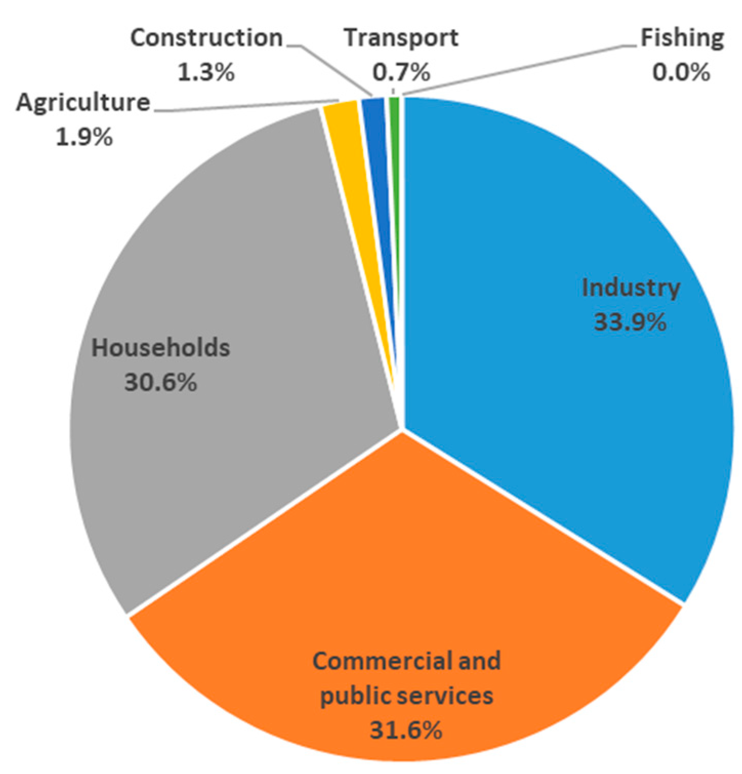
They represent the main areas of the economy, i.e., industry output (industrial production), trade volume (wholesale and retail trade, repair of motor vehicles and motorcycles, exports, exports of goods of Lithuanian origin and imports), prices (consumer price changes), labor market (unemployment), and expectations (consumer confidence and economic sentiment indicator). Three electricity market data, i.e., electricity consumption, electricity production, and electricity price, are analyzed as potential high-frequency regressors to nowcast the macroeconomic indicators. Based on data from Statistics Lithuania of 2021, industry is the largest consumer of electricity. It accounts for 34% of the final consumption. Meanwhile, companies of commercial and public services form the second largest group of electricity consumers (Figure 1).

The primary analysis covers the monthly electricity market (aggregated daily data) and macroeconomic data to find the relationship between them. The stationarity of time series is tested using augmented Dickey–Fuller (ADF) and Phillips–Perron (PP) tests. Phillips and Perron (1988) propose an alternative (nonparametric) method for controlling for serial correlation when testing for a unit root. The direction of the relationship between indicators is tested using the Granger causality test.

The mixed data sampling (MIDAS) regression model (Bai et al. 2013) is applied to nowcast macroeconomic indicators based on electricity market data. MIDAS lets you overcome the problem of data with mixed frequency. It also allows you to minimize the number of estimated parameters and make the regression model simpler. Before the introduction of the MIDAS model, a commonly used approach was to average the high-frequency observations using equal weights to obtain aggregated regressors measured at the same low frequency as the dependent variable. However, this assumption sometimes leads to high forecast errors. The MIDAS framework introduced by Ghysels et al. (2004) comprises diverse lag structures that are employed to parameterize the regression model. A weighting function, which can have a number of functional forms, is used to reduce the number of parameters in the MIDAS regression (Utari and Ilma 2018). The methodology of MIDAS is described in detail by Toker et al. (2022), (Ghysels et al. 2020), and others. The following MIDAS specifications are used in this research:

• Step weighting. In general, it employs the step function:

  $$y_t=X_t^{\prime }\beta +{{\displaystyle \sum }}_{\tau =0}^{k-1}{X}_{\left(t-\tau \right)/S^{\prime }}^H{\phi }_{\tau }+{ϵ}_t$$

  (1)

  In this research, y_t is a macroeconomic indicator, $X_{\left(t-\tau \right)/S}^H$ are electricity market indicators, S is number of values for each low-frequency value, and β and φ_τ are parameters to be estimated. The lag value of y_t is included in place of $X_t^{\prime }$. It is chosen based on the delay period of each macroeconomic indicator, and the maximum number of days of delay is taken. k is the number of high-frequency lags to be included in the low-frequency regression equation, and it is also set to the maximum delay period. The step length is set to 7 days. Therefore, every seven lags of the electricity market indicators $X_{\left(t-\tau \right)/S}^H$ employ the same coefficient.
• Almon weighting. Almon lag weighting is also called polynomial distributed lag (PDL) weighting and is widely used to place restrictions on lag coefficients in autoregressive models. The model can be written as:

  $$y_t=X_t^{\prime }\beta +{{\displaystyle \sum }}_{\tau =0}^{k-1}{X}_{\left(t-\tau \right)/S^{\prime }}^H\left({{\displaystyle \sum }}_{j=0}^p{\tau }^j{\theta }_j\right)+{ϵ}_t$$

  (2)

  P is Almon polynomial order. The coefficients are modelled as a p dimensional lag polynomial in the MIDAS parameters θ for each high-frequency lag up to k.
• Beta weighting. It is based on the normalized beta weighting function and was introduced by Ghysels, Santa-Clara, and Valkanov (Ghysels et al. 2004):

  $$y_t=X_t^{\prime }\beta +{{\displaystyle \sum }}_{\tau =0}^{k-1}{X_{\left(t-\tau \right)}^H}^{\prime }\left(\frac{{\mathrm{w}}_{\tau }^{{\theta }_1-1}{\left(1-w_{\tau }\right)}^{{\theta }_2-1}}{{{\displaystyle \sum }}_{j=0}^k{\mathrm{w}}_j^{{\theta }_1-1}{\left(1-w_j\right)}^{{\theta }_2-1}}+{\theta }_3\right)\lambda +{ϵ}_t$$

  (3)

  $$w_i=\left\{\begin{array}{c}\sigma i=0\\ i/\left(k-1\right) i=1,\dots ,k-2\\ 1-\delta i=k\end{array}\right.$$

  (4)

  σ is a small number (in practice, approximately equal to 2.22 × 10⁻¹⁶). The beta function is very flexible and can take many shapes depending on the values of the parameters θ₁, θ₂, and θ₃. The restriction θ₃ = 0 is used, which means that there are zero weights at the high-frequency lag endpoints.
• U-MIDAS. This is unrestricted MIDAS regressions. This technique adds each of the higher-frequency components as a regressor in the lower-frequency regression and is simply the individual coefficients method given by Equation (1).
• Auto/GETS weighting. It is an extension of U-MIDAS that uses variable selection to reduce the number of individual coefficients by excluding individual lags.

Monthly macroeconomic data are announced with a delay (

Table 1. Delay of macroeconomic indicators.

Macroeconomic Indicator	Delay, in Days
Unemployment rate	30–60
Consumer confidence	0–30
Economic sentiment indicator	0–36
Exports	39–69
Exports of goods of Lithuanian origin	39–69
Imports	39–69
CPI-based consumer price changes	8–39
Industrial production	22–53
Wholesale and retail trade, repair of motor vehicles and motorcycles	26–57

). For example, the unemployment rate is announced at the end of the next month. Therefore, if we take, for example, November 30, the unemployment rate for October is already known (30 days’ delay), but only the unemployment rate for September is known until November 29 (60 days delay). Expectation indicators have the shortest delay (approximately up to 1 month). Meanwhile, exports and imports are announced with the greatest delay (up to 70 days). Delay period is taken into account when choosing lags for low- and high-frequency variables.

The estimation sample runs from January 2010 to December 2019 to obtain reliable parameter estimates. Then, the forecasting of the economic indicators for the next 34 months, from January 2020 to October 2022, is conducted. The results of the MIDAS regression are compared with the predictions using the autoregressive function (AR). Symmetric mean absolute percentage error (SMAPE) is used as an accuracy measure. It is based on percentage errors and is calculated as follows:

$$\mathrm{SMAPE}=\frac{100\%}{n}{{\displaystyle \sum }}_{t=1}^n\frac{\left|{\widehat{y}}_t-y_t\right|}{\left(\left|{\widehat{y}}_t\right|+\left|y_t\right|\right)/2}$$

(5)

where ${\widehat{y}}_t$ is the forecast value, and y_t is the actual value. SMAPE is a modified MAPE often used to avoid dealing with an unbounded metric. In addition to SMAPE, mean absolute error (MAE) and root mean square error (RMSE) are used as alternative accuracy measures to obtain robust results.

$$\mathrm{MAE}=\frac{1}{n}{{\displaystyle \sum }}_{t=1}^n\left|{\widehat{y}}_t-y_t\right|$$

(6)

$$\mathrm{RMSE}=\sqrt{{{\displaystyle \sum }}_{t=1}^n\frac{{\left({\widehat{y}}_t-y_t\right)}^2}{n}}$$

(7)

A significance level of 0.05 is used to test the hypotheses. EViews software is employed for the calculations.

4. Results and Discussion

The descriptive statistics of the monthly indicators investigated are presented in

Table 2. Descriptive statistics and order of integration.

Indicator	Mean	Median	Maximum	Minimum	Std. Dev.	No. of Observations	Order of Integration
Electricity consumption	890,154	871,866	1,235,045	705,755	116,988	154	I(0)
Electricity production	305,104	298,734	726,674	127,108	91,651	154	I(0)
Electricity price	63.16	44.51	480.36	23.31	63.85	118	I(1)
Unemployment rate	9.84	8.60	18.70	5.10	3.76	154	I(0)
Economic sentiment indicator	−0.63	−0.80	11.30	−26.00	6.67	118	I(0)
Consumer confidence	−6.36	−5.00	8.00	−34.00	8.06	154	I(0)
Imports	2,382,542	2,266,725	5,240,538	1,033,667	667,428	153	I(1)
Exports	2,179,279	2,064,967	4,410,498	900,511	571,224	153	I(1)
Exports of goods of Lithuanian origin	1,330,753	1,256,003	2,615,594	670,780	343,840	153	I(1)
Consumer price changes	0.32	0.20	2.90	−1.30	0.65	154	I(0)
Industrial production	1,818,556	1,679,641	3,641,898	1,155,882	460,838	154	I(1)
Wholesale and retail trade, repair of motor vehicles and motorcycles	2,838,063	2,635,202	5,722,806	1,195,498	904,126	153	I(0)

. Both ADF and PP tests provide evidence that electricity production, unemployment rate, economic sentiment indicator, consumer confidence, and consumer price changes are stationary time series (without trend and constant). Electricity consumption is also stationary if constant is included, while wholesale and retail trade is stationary if constant and linear trend is included. All other indicators are first-order integrated processes based on ADF and PP tests.

As all indicators are I(0) and I(1) processes, they are differenced once to check the simultaneous (based on correlation analysis) and delayed (based on Granger causality test) relationship between them. According to the correlation analysis, the electricity consumption is significantly correlated (at a significance level of 0.05) with the unemployment rate, consumer confidence, exports, exports of goods of Lithuanian origin, and industrial production. Electricity production is significantly correlated only with industrial production. Meanwhile, electricity price is significantly correlated with all trade indicators (wholesale and retail trade, repair of motor vehicles and motorcycles, exports, exports of goods of Lithuanian origin and imports) and with industrial production (

Table 3. Correlation matrix.

Correlation Probability	d(Electricity Consumption)	d(Electricity Production)	d(Electricity Price)	d(Unemployment Rate)	d(Economic Sentiment)	d(Consumer Confidence)	d(Imports)	d(Exports)	d(Lithuanian Exports)	d(Consumer Price Changes)	d(Industrial Production)	d(Trade)
d(Electricity consumption)	1.0000
	-----
d(Electricity production)	0.3153	1.0000
	0.0001	-----
d(Electricity price)	0.2314	0.0884	1.0000
	0. 0121	0.3434	-----
d(Unemployment rate)	0.1589	0.0959	0.0274	1.0000
	0.0497	0.2381	0.7691	-----
d(Economic sentiment)	−0.0203	−0.0930	0.0422	−0.1914	1.0000
	0.8284	0.3185	0.6511	0.0387	-----
d(Consumer confidence)	0.1728	−0.0048	0.0462	−0.0008	0.6186	1.0000
	0.0327	0.9535	0.6211	0.9925	0.0000	-----
d(Imports)	0.1415	0.1229	0.2201	−0.0834	0.0858	−0.0131	1.0000
	0.0820	0.1314	0.0176	0.3069	0.3597	0.8725	-----
d(Exports)	0.1751	0.1210	0.3111	−0.0167	0.1681	0.0288	0.8031	1.0000
	0.0309	0.1375	0.0007	0.8382	0.0712	0.7248	0.0000	-----
d(Lithuanian exports)	0.2743	0.1488	0.3349	−0.0706	0.2098	0.1047	0.6507	0.8712	1.0000
	0.0006	0.0672	0.0002	0.3871	0.0238	0.1993	0.0000	0.0000	-----
d(Consumer price changes)	−0.0408	0. 1239	0.0085	−0.0357	0.1038	0.0135	0.1190	0.0804	0.1480	1.0000
	0.6165	0.1270	0.9277	0.6615	0.2654	0.8687	0.1442	0.3251	0.0689	-----
d(Indus-trial production)	0.4889	0.2885	0.3217	0.0535	0.0261	0.0514	0.7279	0.8037	0.8247	0.0867	1.0000
	0.0000	0.0003	0.0004	0.5110	0.7803	0.5283	0.0000	0.0000	0.0000	0.2864	-----
d(Trade)	0.1044	0.1423	0.2536	0.0869	0.0275	−0.0790	0.6368	0.6796	0.4286	0.1109	0.5246	1.0000
	0.2004	0. 0802	0.0060	0.2869	0.7693	0.3331	0.0000	0.0000	0.0000	0.1738	0.0000	-----

).

The Granger causality test shows that electricity consumption and electricity price Granger cause all investigated macroeconomic indicators, except the unemployment rate and expectations (

Table 4. Results of Granger causality test.

Indicator	l = 1	l = 2	l = 3	l = 4	l = 5	l = 6
H0: d(Electricity consumption) does not Granger cause an indicator
d(Unemployment rate)	0.5444	0.2606	0.3008	0.8114	0.8252	0.5561
d(Economic sentiment indicator)	0.7170	0.7203	0.5004	0.4717	0.5354	0.7884
d(Consumer confidence)	0.7003	0.8479	0.9626	0.8587	0.8954	0.8205
d(Imports)	0.0000	0.0000	0.0001	0.0003	0.0000	0.0000
d(Exports)	0.0000	0.0001	0.0005	0.0001	0.0002	0.0000
d(Exports of goods of Lithuanian origin)	0.0207	0.0178	0.0884	0.0031	0.0050	0.0000
d(Consumer price changes)	0.9754	0.1983	0.0017	0.0034	0.0042	0.0000
d(Industrial production)	0.0016	0.0024	0.0118	0.0044	0.0041	0.0002
d(Wholesale and retail trade)	0.0000	0.0000	0.0000	0.0000	0.0000	0.0000
H0: d(Electricity production) does not Granger cause an indicator
d(Unemployment rate)	0.7086	0.5693	0.1664	0.3729	0.0503	0.0067
d(Economic sentiment indicator)	0.1155	0.0903	0.2573	0.0925	0.1312	0.0689
d(Consumer confidence)	0.5286	0.0279	0.0320	0.0425	0.0338	0.1185
d(Imports)	0.7556	0.6399	0.9029	0.5149	0.0515	0.0829
d(Exports)	0.5696	0.1906	0.4223	0.0149	0.0026	0.0033
d(Exports of goods of Lithuanian origin)	0.3589	0.4827	0.6630	0.0462	0.0027	0.0029
d(Consumer price changes)	0.0654	0.2251	0.1309	0.1024	0.3645	0.5179
d(Industrial production)	0.3239	0.4406	0.5099	0.1586	0.0060	0.0109
d(Wholesale and retail trade)	0.0779	0.0990	0.0749	0.0568	0.0059	0.0106
H0: d(Electricity price) does not Granger cause an indicator
d(Unemployment rate)	0.6487	0.8959	0.8688	0.7986	0.8010	0.8328
d(Economic sentiment indicator)	0.5471	0.8762	0.4692	0.5509	0.6810	0.6919
d(Consumer confidence)	0.0813	0.1990	0.1005	0.1640	0.1931	0.2463
d(Imports)	0.1413	0.2174	0.0014	0.0006	0.0024	0.0004
d(Exports)	0.2464	0.1345	0.0261	0.0052	0.0105	0.0003
d(Exports of goods of Lithuanian origin)	0.3012	0.4508	0.1616	0.0202	0.0118	0.0000
d(Consumer price changes)	0.0263	0.2891	0.0470	0.2423	0.1797	0.0047
d(Industrial production)	0.7867	0.9456	0.0001	0.0000	0.0000	0.0000
d(Wholesale and retail trade)	0.9589	0.9975	0.0529	0.0561	0.0852	0.0367

). The causality between electricity price and wholesale and retail trade and repair of motor vehicles and motorcycles appears only when six lags are included. Meanwhile, electricity production Granger causes all investigated macroeconomic indicators, except the economic sentiment indicator, imports, and consumer price changes.

4.1. Nowcasting Unemployment Rate

Based on the correlation and causality analysis, the unemployment rate significantly correlates with electricity consumption and is Granger caused by electricity production when lag is 6. Thus, electricity consumption and production will be analyzed as high-frequency regressors. Since the unemployment rate is announced with a maximum of 60 days’ delay, the 60 days’ lagged value of the unemployment rate is included to account for its actual value, and the 60 lagged values of electricity consumption and production are included in the MIDAS model as high-frequency regressors. The error metrics of the MIDAS models are presented in

Table 5. Errors of modified AR(2) and MIDAS models.

Model Included High-Frequency Variables	Error Metrics	Step Weighting	Almon (PDL) Weighting: Polynomial Degree: 2	Almon (PDL) Weighting: Polynomial Degree: 3	Beta Weighting	U-MIDAS	Auto/GETS Weighting
Electricity consumption	RMSE MAE SMAPE	0.9162 0.7188 9.6339	0.9151 0.7179 9.6192	0.9159 0.7187 9.6358	0.9254 0.7322 9.8156	0.9178 0.7213 9.6757	0.9172 0.7210 9.6689
Electricity production	RMSE MAE SMAPE	0.9045 0.6948 9.3092	0.8710 0.6687 8.9896	0.9048 0.6963 9.3258	0.8927 0.6889 9.2496	0.9076 0.6965 9.3305	0.9036 0.6940 9.3017
Electricity consumption and production	RMSE MAE SMAPE	0.9509 0.7341 9.6605	0.9377 0.7296 9.6221	0.9485 0.7347 9.6745	0.9488 0.7388 9.8660	0.9502 0.7357 9.6826	0.9498 0.7355 9.6866
Modified AR(2)	RMSE MAE SMAPE	0.7474 0.6367 8.7458

. The results are compared with those obtained by the autoregressive function. The modified AR(2) model, that is, y_t = f(y_t−2), not including y_t−1, is analyzed to evaluate the benefit of the electricity market indicators to nowcast the unemployment rate.

Electricity production gives slightly lower RMSE, MAE, and SMAPE than electricity consumption in all models. The inclusion of both electricity market indicators does not improve the precision. If only electricity production is included as a high-frequency variable, Almon (PDL) weighting with polynomial degree 2 provides the lowest errors. However, the results of all the methods show that none of these two electricity market indicators improve the prediction of the unemployment rate compared with the prediction by the modified AR(2) model.

4.2. Nowcasting Consumer Confidence

Consumer confidence significantly correlates with electricity consumption and is Granger caused by the electricity production. Thus, these two electricity market indicators will be analyzed as high-frequency regressors. As consumer confidence is announced with a maximum of 30 days’ delay, a 30 days’ lagged value of consumer confidence is included to account for its actual value, and the 30 lagged values of electricity production and consumption are included as high-frequency regressors in the MIDAS model. The error metrics of MIDAS models are presented in

Table 6. Errors of AR(1) and MIDAS models.

Model Included High-Frequency Variables	Error Metrics	Step Weighting	Almon (PDL) Weighting: Polynomial Degree: 2	Almon (PDL) Weighting: Polynomial Degree: 3	Beta Weighting	U-MIDAS	Auto/GETS Weighting
Electricity consumption	RMSE MAE SMAPE	3.8107 2.5008 86.7487	3.8014 2.5067 88.2265	3.8132 2.5000 86.7099	3.8216 2.5137 87.9180	3.8175 2.5014 86.3413	3.8227 2.5043 86.3871
Electricity production	RMSE MAE SMAPE	3.7807 2.6036 93.3369	3.7813 2.6099 93.5773	3.7793 2.6021 93.2429	3.7736 2.6051 93.3055	3.7819 2.6045 93.3162	3.7758 2.5998 92.8436
Electricity consumption and production	RMSE MAE SMAPE	3.8116 2.6468 94.8711	3.8069 2.6585 95.8081	3.8144 2.6476 94.9884	3.7917 2.5607 90.5334	3.8188 2.6457 94.6325	3.8255 2.6466 94.1913
AR(1)	RMSE MAE SMAPE	3.8018 2.5503 89.3181

. The results are compared with the predictions of the AR(1) model y_t = f(y_t−1) as the consumer confidence has a delay of 1 month.

The results show that the most appropriate method and selection of the high-frequency variables vary depending on the chosen error metrics. On the basis of MAE and SMAPE, the inclusion of electricity consumption provides the highest precision. Meanwhile, RMSE is the lowest if electricity production is included. If only electricity consumption is included, MAE indicates the Almon (PDL) weighting method when the polynomial degree is 3 being the most accurate, while U-MIDAS is the most suitable method based on SMAPE. Both cases provide just slightly lower errors compared with AR(1).

4.3. Nowcasting Economic Sentiment Indicator

The economic sentiment indicator does not correlate significantly with any of the electricity market indicators and is not Granger caused by any of them. Therefore, changes in the economic sentiment indicator cannot be explained by the electricity market indicators.

4.4. Nowcasting Exports

Exports significantly correlate with the electricity consumption and price, and are Granger caused by all three electricity market indicators. The causality with electricity production is seen only after approximately 4 months. As exports are announced with a maximum of 69 days’ delay, a 69 days’ lagged value of exports is included to account for its actual value, and the 69 lagged values of electricity market indicators are included in the MIDAS model as high-frequency regressors. The error metrics of MIDAS models are presented in

Table 7. Errors of modified AR(2) and MIDAS models.

Model Included High-Frequency Variables	Error Metrics	Step Weighting	Almon (PDL) Weighting: Polynomial Degree: 2	Almon (PDL) Weighting: Polynomial Degree: 3	Beta Weighting	U-MIDAS	Auto/GETS Weighting
Electricity consumption	RMSE MAE SMAPE	455,945 365,603 12.8055	455,233 365,169 12.7881	456,714 366,325 12.8288	464,425 372,077 13.0131	455,741 365,576 12.8044	456,429 365,846 12.8070
Electricity production	RMSE MAE SMAPE	491,984 399,114 14.0384	488,488 394,817 13.8692	491,246 398,383 14.0082	491,178 397,743 13.9728	492,452 399,681 14.0607	490,543 397,324 13.9614
Electricity price	RMSE MAE SMAPE	314,133 276,658 9.9670	310,831 274,555 9.9063	312,112 275,331 9.9291	302,559 271,663 9.8586	317,002 278,567 10.0142	308,625 271,218 9.8807
Electricity price and consumption	RMSE MAE SMAPE	414,275 330,644 10.9346	405,986 327,406 10.8275	412,582 329,591 10.9086	338,208 290,853 10.4921	418,202 332,447 10.9746	380,743 313,946 10.6020
Modified AR(2)	RMSE MAE SMAPE	450,302 356,616 12.4634

. The results are compared with the prediction using the modified AR(2) model y_t = f(y_t−2), not including y_t−1 (because exports are announced with a 2-month delay), in order to evaluate the benefit of electricity market indicators to nowcast exports.

Electricity price is the best predictor among the three indicators of the electricity market. A combination of several economic market indicators does not improve the precision. Moreover, electricity price improves the prediction of export compared with the modified AR(2) model. Nowcasting exports by electricity price using the beta weighting method gives the lowest SMAPE (9.86%) and RMSE. The lowest MAE is got using the Auto/GETS weighting method.

4.5. Nowcasting Exports of Goods of Lithuanian Origin

Exports of goods of Lithuanian origin also significantly correlate with the electricity consumption and price and are Granger caused by all three electricity market indicators. As exports of goods of Lithuanian origin are announced with a maximum of 69 days’ delay, a 69 days’ lagged value of the dependent variable is included to account for its actual value, and the 69 lagged values of electricity market indicators are included in the MIDAS model as high-frequency regressors. The error metrics of MIDAS models are presented in

Table 8. Errors of modified AR(2) and MIDAS models.

Model Included High-Frequency Variables	Error Metrics	Step Weighting	Almon (PDL) Weighting: Polynomial Degree: 2	Almon (PDL) Weighting: Polynomial Degree: 3	Beta Weighting	U-MIDAS	Auto/GETS Weighting
Electricity consumption	RMSE MAE SMAPE	311,214 249,809 14.3337	307,917 247,461 14.2065	310,786 249,179 14.2971	310,041 249,044 14.2829	311,740 250,226 14.3559	311,196 249,809 14.3285
Electricity production	RMSE MAE SMAPE	319,899 263,628 15.2377	317,563 259,786 14.9875	319,375 263,170 15.2090	324,357 268,352 15.5558	320,096 263,947 15.2590	321,014 264,817 15.3245
Electricity price	RMSE MAE SMAPE	235,221 199,113 11.3411	232,658 197,223 11.2910	234,854 197,802 11.2903	210,438 179,967 10.4422	236,641 199,835 11.3630	224,824 189,778 10.9809
Electricity price and consumption	RMSE MAE SMAPE	275,107 220,718 11.9430	267,422 212,676 11.5294	271,170 217,426 11.7991	346,051 273,638 15.5648	277,904 222,523 12.0165	256,540 208,081 11.4586
Modified AR(2)	RMSE MAE SMAPE	289,595 228,748 13.1592

. The results are compared with the predictions using the modified AR(2) model y_t = f(y_t−2), not including y_t−1 (because exports of goods of Lithuanian origin are announced with a delay of 2 months), in order to evaluate the benefit of electricity market indicators to nowcast the exports of goods of Lithuanian origin.

Electricity price is the best predictor among the three indicators of the electricity market. The inclusion of any other electricity market indicator does not improve the prediction. Nowcasting exports of goods of Lithuanian origin by electricity price using the beta weighting method gives the lowest error, and it provides better results than the modified AR(2) model.

4.6. Nowcasting Imports

Imports significantly correlate with the electricity price and are Granger caused by electricity consumption and price. As imports are announced with a maximum of 69 days’ delay, a 69 days’ lagged value of the dependent variable is included to account for its actual value, and the 69 lagged values of electricity market indicators are included in the MIDAS model as high-frequency regressors. The error metrics of MIDAS models are presented in

Table 9. Errors of modified AR(2) and MIDAS models.

Model Included High-Frequency Variables	Error Metrics	Step Weighting	Almon (PDL) Weighting: Polynomial Degree: 2	Almon (PDL) Weighting: Polynomial Degree: 3	Beta Weighting	U-MIDAS	Auto/GETS Weighting
Electricity consumption	RMSE MAE SMAPE	586,580 453,913 14.3131	585,508 452,626 14.2614	588,066 454,250 14.3162	604,184 468,836 14.6829	586,315 453,805 14.3103	587,298 454,637 14.3313
Electricity price	RMSE MAE SMAPE	566,552 449,927 14.1709	553,270 441,618 13.8965	561,430 448,013 14.0911	537,808 430,359 13.6044	568,252 452,366 14.2472	579,460 460,907 14.4646
Electricity price and consumption	RMSE MAE SMAPE	416,348 340,265 11.2080	381,638 308,322 10.3410	409,549 335,361 11.0905	580,363 464,490 14.4943	418,805 342,330 11.2589	434,113 355,546 11.6417
Modified AR(2)	RMSE MAE SMAPE	580999 443028 13.9565

. The results are compared with the predictions using the modified AR(2) model y_t = f(y_t−2), not including y_t−1.

In this case, the electricity price is also the best predictor between these two electricity market indicators, but electricity price and consumption together let you improve the prediction the most. Nowcasting imports by two electricity market indicators using the Almon (PDL) weighting method when the polynomial degree is 2 provide the lowest errors, and they improve the prediction in comparison with the modified AR(2) model.

4.7. Nowcasting CPI-Based Consumer Price Changes

CPI-based consumer price changes do not significantly correlate with any of the electricity market indicators, but are Granger caused by electricity consumption and electricity price. As CPI-based consumer price changes are announced with a maximum of 39 days’ delay, a 39 days’ lagged value of the dependent variable is included to account for its actual value, and the 39 lagged values of electricity market indicators are included in the MIDAS model as high-frequency regressors. Errors of MIDAS models are presented in

Table 10. Errors of AR(1) and MIDAS models.

Model Included High-Frequency Variables	Error Metrics	Step Weighting	Almon (PDL) Weighting: Polynomial Degree: 2	Almon (PDL) Weighting: Polynomial Degree: 3	Beta Weighting	U-MIDAS	Auto/GETS Weighting
Electricity consumption	RMSE MAE SMAPE	0.9527 0.7303 120.4018	0.9532 0.7312 119.8994	0.9509 0.7282 119.6651	0.9428 0.7169 113.9689	0.9515 0.7298 120.0368	0.9549 0.7315 120.4331
Electricity price	RMSE MAE SMAPE	2.5303 1.7425 174.8308	2.5455 1.7622 175.1857	2.5270 1.7410 174.7358	2.5490 1.7568 174.8233	2.5275 1.7391 174.7478	2.4254 1.6743 174.1631
Electricity consumption and price	RMSE MAE SMAPE	2.4291 1.6555 163.3825	2.4409 1.6672 162.5086	2.4163 1.6458 163.0349	1.6237 1.1595 154.2820	2.3853 1.6290 163.0523	2.3214 1.5928 163.3037
AR(1)	RMSE MAE SMAPE	0.9094 0.6772 114.8734

. The results are compared with predictions using the AR(1) model y_t = f(y_t−1) as the CPI-based consumer price changes are announced with approximately 1-month delay.

The electricity price performs the worst even if the maximum lag is increased. Electricity consumption performs better, but it does not improve the prediction of CPI-based consumer price changes compared with AR(1) based on RMSE and MAE. Only the SMAPE of the beta weighting model is slightly lower than the SMAPE of AR(1).

4.8. Nowcasting Industrial Production

Industrial production is significantly correlated and Granger caused by all three electricity market indicators. Thus, all three indicators of the electricity market are analyzed as regressors. As industrial production is announced with a maximum of 53 days’ delay, a 53 days’ lagged value of the dependent variable is included to account for its actual value, and the 53 lagged values of electricity market indicators are included in the MIDAS model as high-frequency regressors. Errors of MIDAS models are presented in

Table 11. Errors of modified AR(2) and MIDAS models.

Model Included High-Frequency Variables	Error Metrics	Step Weighting	Almon (PDL) Weighting: Polynomial Degree: 2	Almon (PDL) Weighting: Polynomial Degree: 3	Beta Weighting	U-MIDAS	Auto/GETS Weighting
Electricity consumption	RMSE MAE SMAPE	379,730 279,626 11.2332	377,725 278,149 11.1745	379,625 279,652 11.2366	380,562 280,463 11.2647	380,209 279,808 11.2374	380,121 279,670 11.2317
Electricity production	RMSE MAE SMAPE	353,353 259,924 10.5062	352,805 259,158 10.4776	353,148 259,782 10.5028	345,049 251,454 10.1210	353,445 260,243 10.5196	354,461 261,271 10.5697
Electricity price	RMSE MAE SMAPE	289,410 216,678 8.9000	290,894 214,488 8.8274	289,577 216,110 8.8804	265,535 197,893 8.2428	290,774 217,498 8.9315	285,210 212,603 8.7710
Electricity production and price	RMSE MAE SMAPE	299,661 221,423 8.9961	305,900 222,047 9.0002	300,579 220,877 8.9644	295,252 214,106 8.7085	300,727 222,271 9.0290	291,054 215,231 8.7993
Electricity consumption, production, and price	RMSE MAE SMAPE	279,899 205,096 8.4420	287,570 209,066 8.5580	281,291 205,560 8.4537	263,542 191,519 7.9054	280,429 206,338 8.4822	274,060 201,221 8.3163
Modified AR(2)	RMSE MAE SMAPE	373,471 283,334 11.5615

. The results are compared with the precision of the modified AR(2) model y_t = f(y_t−2) without y_t−1 in order to evaluate the benefit of electricity market indicators to nowcast the industrial production.

In general, any electricity market indicator lets you improve the prediction of industrial production compared with the modified AR(2) model, except that the RMSE of nowcasts based on electricity consumption is a bit higher. Electricity price performs best among them, but the inclusion of all three electricity market indicators lets you reduce the errors the most. Nowcasting industrial production by three electricity market indicators using beta weighting gives the lowest SMAPE (7.91%), MAE, and RMSE.

4.9. Nowcasting Wholesale and Retail Trade, Repair of Motor Vehicles and Motorcycles

Wholesale and retail trade and repair of motor vehicles and motorcycles significantly correlate with electricity price and is Granger caused by all three electricity market indicators. Thus, three indicators of the electricity market are analyzed as regressors. Like wholesale and retail trade, the repair of motor vehicles and motorcycles is announced with a maximum of 57 days’ delay, a 57-day lagged value of the dependent variable is included to account for its actual value, and the 57-day lagged values of the electricity market indicators are included in the MIDAS model as high-frequency regressors. The error metrics of MIDAS models are presented in

Table 12. Errors of modified AR(2) and MIDAS models.

Model Included High-Frequency Variables	Error Metrics	Step Weighting	Almon (PDL) Weighting: Polynomial Degree: 2	Almon (PDL) Weighting: Polynomial Degree: 3	Beta Weighting	U-MIDAS	Auto/ GETS Weighting
Electricity consumption	RMSE MAE SMAPE	490,105 407,913 10.3014	490,474 410,223 10.3643	492,261 411,054 10.3900	528,777 434,912 10.9728	489,344 406,572 10.2666	489,940 407,037 10.2775
Electricity production	RMSE MAE SMAPE	572,953 480,521 12.1206	570,672 478,732 12.0788	573,001 480,871 12.1303	572,539 480,029 12.1114	573,276 480,912 12.1318	569,469 476,925 12.0288
Electricity price	RMSE MAE SMAPE	824,322 646,186 16.0939	820,388 649,943 16.1344	815,554 639,747 15.9311	826,042 645,457 16.0328	825,428 647,064 16.1175	766,679 610,801 15.1843
Electricity consumption and production	RMSE MAE SMAPE	514,576 433,943 10.9762	515,226 436,936 11.0565	518,658 439,320 11.1214	573,328 494,405 12.3684	512,053 431,238 10.9062	509,925 428,729 10.8395
Modified AR(2)	RMSE MAE SMAPE	553,927 465,897 11.7100

. The results are compared with those obtained by the autoregressive function. As there is an almost 2-month delay, the modified AR(2) model y_t = f(y_t−2) not including y_t−1 is used to forecast wholesale and retail trade and the repair of motor vehicles and motorcycles. Its errors are compared with the errors of MIDAS models in order to evaluate the benefit of electricity market indicators to nowcast wholesale and retail trade and the repair of motor vehicles and motorcycles.

Electricity production and price do not improve the prediction of wholesale and retail trade and the repair of motor vehicles and motorcycles compared with the modified AR(2) model. Meanwhile, electricity consumption is the most suitable predictor, and the U-MIDAS model performs the best. It provides the lowest RMSE, MAE, and SMAPE values.

4.10. Comparison of Real and Nowcasted Values

A comparison of the real values of macroeconomic indicators (blue line) and their predicted values based on electricity market data using the best MIDAS models are presented in Figure 2. Calculations showed that exports and exports of goods of Lithuanian origin can be best nowcasted by the electricity price using the beta weighting method. Meanwhile, imports can be best nowcasted by electricity price and consumption using the Almon (PDL) weighting method when the polynomial degree is 2. As can be seen from the charts, signals about the changes in trade are lagging behind because the lag value of the dependent variable is included in the model, which dominates and allows for significantly improving the precision of the forecasts. However, electricity market indicators warn of these changes in trade indicators earlier and show a significant decline in international trade and in industrial production in October.

Nowcasts of industrial production by all three electricity market indicators using the beta weighting method provide quite accurate warnings about the changes in industrial production. Meanwhile, the nowcasts of consumer confidence and wholesale and retail trade and the repair of motor vehicles and motorcycles by electricity consumption using the U-MIDAS model just slightly outperform the autoregressive model. Their performance is compared with the AR(1) predictions. It is obvious that the electricity market data do not significantly improve the prediction. Meanwhile, the unemployment rate and CPI-based consumer price changes are not nowcasted as electricity market data do not improve the prediction compared with the autoregressive model.

In summary, the electricity market data are a good representative of the direction the economy is going, indicating the changes in the output. We found that electricity consumption is the most useful to nowcast economic activity. These results are in line with Lehmann and Sascha (2022), Wegmüller et al. (2023), and Fezzi and Fanghella (2021), who identified a close relationship between GDP growth and electricity consumption in big economies and Nordic and Central European countries. We showed that electricity consumption is the most useful indicator in nowcasting economic activity in small open economy as well. Electricity price is the most useful to nowcast exports, exports of goods of Lithuanian origin, imports, and industrial production. These findings are similar to the results obtained by Knotek and Zaman (2017), who identified that high-frequency energy price data play a key role in improving nowcasting accuracy.

However, various shocks, such as war in Ukraine and sharp spikes in electricity prices in August and September, can change the relationship between electricity market data and macroeconomic indicators, causing larger errors. Thus, a review and renewal of the model in such cases is needed. The analysis of model sensitivity and its changes based on economic situations (decline, growth, or in the case of various economic shocks) will be analyzed in further research.

5. Conclusions

In general, electricity market indicators are useful to nowcast macroeconomic indicators, but they perform differently depending on the macroeconomic indicator that is aimed to nowcast. Electricity consumption is the most useful among the three analyzed electricity market indicators and brings benefits when nowcasting imports, industrial production, consumer confidence, wholesale and retail trade, and the repair of motor vehicles and motorcycles. Electricity production is also beneficial for nowcasting industrial production. Meanwhile, electricity price is useful to nowcast exports, exports of goods of Lithuanian origin, imports, and industrial production. However, electricity market data do not improve the prediction of the unemployment rate, economic sentiment indicator, and CPI-based consumer price compared with the autoregressive model.

Withal, the precision of the MIDAS models differs. Industrial production can be nowcasted most accurately with a SMAPE of 7.9%. The SMAPE of nowcasts of exports, exports of goods of Lithuanian origin, imports, wholesale and retail trade, and the repair of motor vehicles and motorcycles is around 10%. Meanwhile, for all other economic indicators, the SMAPE exceeds 86%, except that the nowcasting unemployment rate provides lower errors, but the ability of electricity market indicators to nowcast the unemployment rate is low. The U-MIDAS, Almon (PDL) weighting, and beta weighting methods in most cases provide the most accurate results.

In general, the results of this research confirm the links between the electricity market and the entire economy. Electricity is one of the most important resources of companies. Thus, its usage reflects the scope of economic activity. Hence, the fact that electricity consumption allows for nowcasting industrial production, as well as wholesale and retail trade and the repair of motor vehicles and motorcycles, is not surprising. Since production is sold in the local market and exported, electricity consumption also reflects volumes of local and international trade. Electricity price, as one of the production and operational resources, adjusts the prices of products and services and modifies the entire volume of production and trade.

The results of this research are useful for the government, businesses, and analysts to study the direction of the economy and to make timely decisions in Lithuania. Other researchers can also benefit when choosing the method or high-frequency indicators to nowcast the economic activity of any other country if such high-frequency data are available.

References

- Angelov, Nikolay, and Daniel Waldenström. 2021. The Impact of COVID-19 on Economic Activity: Evidence from Administrative Tax Registers. IFN Working Paper No. 1397. Stockholm: Research Institute of Industrial Economics. [Google Scholar]
- Bai, Jennie, Eric Ghysels, and Jonathan H. Wright. 2013. State Space Models and MIDAS Regressions. Econometric Reviews 32: 779–813. [Google Scholar] [CrossRef]
- Bańbura, Marta, Domenico Giannone, Michele Modugno, and Lucrezia Reichlin. 2013. Now-Casting and the Real-Time Data Flow. Working Paper Series, No 1564; Frankfurt: European Central Bank. [Google Scholar]
- Barbaglia, Luca, Lorenzo Frattarolo, Luca Onorante, Filippo Maria Pericoli, Marco Ratto, and Luca Tiozzo Pezzoli. 2022. Testing big data in a big crisis: Nowcasting under COVID-19. International Journal of Forecasting, in press. [Google Scholar] [CrossRef]
- Baumeister, Christiane, and James D. Hamilton. 2019. Structural Interpretation of Vector Autoregressions with Incomplete Identification: Revisiting the Role of Oil Supply and Demand Shocks. American Economic Review 109: 1873–910. [Google Scholar] [CrossRef]
- Bennedsen, Mikkel, Eric Hillebrand, and Siem Jan Koopman. 2021. Modeling, forecasting, and nowcasting U.S. CO2 emissions using many macroeconomic predictors. Energy Economics 96: 105118. [Google Scholar] [CrossRef]
- Blanco, Emilio, Laura D’Amato, Fiorella Dogliolo, and María Lorena Garegnani. 2017. Nowcasting GDP in Argentina: Comparing the Predictive Ability of Different Models. Economic Research Working Papers, No. 74. Buenos Aires: Central Bank of Argentina, Economic Research Department. [Google Scholar]
- Blonz, Joshua, and Jacob Williams. 2020. Electricity Demand as a High-Frequency Economic Indicator: A Case Study of the COVID-19 Pandemic and Hurricane Harvey. FEDS Notes. Washington, DC: Board of Governors of the Federal Reserve System. [Google Scholar]
- Carriero, Andrea, Todd E. Clark, and Massimiliano Marcellino. 2020. Nowcasting Tail Risks to Economic Activity with Many Indicators. Federal Reserve Bank of Cleveland, Working Paper No. 20-13R2. Cleveland: Federal Reserve Bank of Cleveland. [Google Scholar]
- Cavallo, Alberto. 2015. Scraped Data and Sticky Prices. National Bureau of Economic Research. Working Paper, No. 21490. Cambridge: National Bureau of Economic Research. [Google Scholar]
- Chen, Kuan-Jen, Angus C. Chu, and Ching-Chong Lai. 2018. Home production and small open economy business cycles. Journal of Economic Dynamics and Control 95: 110–35. [Google Scholar] [CrossRef]
- Cooper, Ilan, and Richard Priestley. 2013. The World Business Cycle and Expected Returns. Review of Finance 17: 1029–106. [Google Scholar] [CrossRef]
- Diaz, Elena Maria, and Gabriel Perez-Quiros. 2021. GEA tracker: A daily indicator of global economic activity. Journal of International Money and Finance 115: 102400. [Google Scholar] [CrossRef]
- Eckert, Florian, Philipp Kronenberg, Heiner Mikosch, and Stefan Neuwirth. 2020. Tracking Economic Activity with Alternative High-Frequency Data. KOF Working Papers, No. 20-488. Zürich: KOF Swiss Economic Institute, ETH Zurich. [Google Scholar]
- Eraslan, Sercan, and Thomas Götz. 2021. An unconventional weekly economic activity index for Germany. Economics Letters 204: 109881. [Google Scholar] [CrossRef]
- Fenz, Gerhard, and Helmut Stix. 2021. Monitoring the economy in real time with the weekly OeNB GDP indicator: Background, experience and outlook. Monetary Policy and the Economy Q4/20–Q1/21: 17–40. [Google Scholar]
- Ferrara, Laurent, and Xuguang Simon Sheng. 2022. Guest editorial: Economic forecasting in times of COVID-19. International Journal of Forecasting 38: 527–28. [Google Scholar] [CrossRef]
- Fezzi, Carlo, and Valeria Fanghella. 2021. Tracking GDP in real-time using electricity market data: Insights from the first wave of COVID-19 across Europe. European Economic Review 193: 103907. [Google Scholar] [CrossRef]
- Ghysels, Eric, Pedro Santa-Clara, and Valkanov Rossen. 2004. The MIDAS Touch: Mixed Data Sampling Regression Models. CIRANO Working Papers 2004s-20. Montreal: CIRANO. [Google Scholar]
- Ghysels, Eric, Virmantas Kvedaras, and Vaidotas Zemlys-Balevičius. 2020. Chapter 4—Mixed data sampling (MIDAS) regression models. In Handbook of Statistics. Edited by Hrishikesh D. Vinod and Calyampudi RadhakrishnaRao. Amsterdam: Elsevier, vol. 42, pp. 117–53. [Google Scholar] [CrossRef]
- Herrera, Ana María, and Sandeep Kumar Rangaraju. 2020. The effect of oil supply shocks on U.S. economic activity: What have we learned? Journal of Applied Econometrics 35: 141–59. [Google Scholar] [CrossRef]
- Huber, Florian, Gary Koop, Luca Onorante, Michael Pfarrhofer, and Josef Schreiner. 2023. Nowcasting in a pandemic using non-parametric mixed frequency VARs. Journal of Econometrics 232: 52–69. [Google Scholar] [CrossRef]
- Kapetanios, George, and Fotis Papailias. 2018. Big Data & Macroeconomic Nowcasting: Methodological Review. Economic Statistics Centre of Excellence (ESCoE), Discussion Papers ESCoE DP-2018-12. London: Economic Statistics Centre of Excellence (ESCoE), King’s Business School, King’s College London. [Google Scholar]
- Kilian, Lutz. 2019. Measuring global real economic activity: Do recent critiques hold up to scrutiny? Economics Letters 178: 106–10. [Google Scholar] [CrossRef]
- Knotek, Edward S., and Saeed Zaman. 2017. Nowcasting US headline and core inflation. Journal of Money, Credit and Banking 49: 931–68. [Google Scholar] [CrossRef]
- Lehmann, Robert, and Möhrle Sascha. 2022. Forecasting Regional Industrial Production with High-Frequency Electricity Consumption Data. CESifo Working Paper No. 9917. Munich: CESifo. [Google Scholar]
- LITGRID. 2022. Available online: https://www.litgrid.eu/index.php/sistemos-duomenys/79 (accessed on 15 December 2022).
- Lourenço, Nuno, and António Rua. 2021. The Daily Economic Indicator: Tracking economic activity daily during the lockdown. Economic Modelling 100: 105500. [Google Scholar] [CrossRef] [PubMed]
- Martins, Bruno Juncklaus, Allan Cerentini, Sylvio Luiz Mantelli, Thiago Zimmermann Loureiro Chaves, Nicolas Moreira Branco, Aldo von Wangenheim, Ricardo Rüther, and Juliana Marian Arrais. 2022. Systematic review of nowcasting approaches for solar energy production based upon ground-based cloud imaging. Solar Energy Advances 2: 100019. [Google Scholar] [CrossRef]
- Mellander, Charlotta, José Lobo, Kevin Stolarick, and Zara Matheson. 2015. Night-Time Light Data: A Good Proxy Measure for Economic Activity? PLoS ONE 10: e0139779. [Google Scholar] [CrossRef]
- Phillips, Peter C. B., and Pierre Perron. 1988. Testing for a Unit Root in Time Series Regression. Biometrika 75: 335–46. [Google Scholar] [CrossRef]
- Proietti, Tommaso, Alessandro Giovannelli, Ottavio Ricchi, Ambra Citton, Christían Tegami, and Cristina Tinti. 2021. Nowcasting GDP and its components in a data-rich environment: The merits of the indirect approach. International Journal of Forecasting 37: 1376–98. [Google Scholar] [CrossRef]
- Sampi, James, and Jooste Charl. 2020. Nowcasting Economic Activity in Times of COVID-19: An Approximation from the Google Community Mobility Report. World Bank Policy Research Working Paper; No. 9247. Washington, DC: The World Bank. [Google Scholar]
- Statistics Lithuania. 2022. Available online: https://osp.stat.gov.lt/statistiniu-rodikliu-analize#/ (accessed on 15 December 2022).
- Toker, Selma, Nimet Özbay, and Kristofer Månsson. 2022. Mixed data sampling regression: Parameter selection of smoothed least squares estimator. Journal of Forecasting 41: 718–751. [Google Scholar] [CrossRef]
- Utari, Dina Tri, and Hafizah Ilma. 2018. Comparison of methods for mixed data sampling (MIDAS) regression models to forecast Indonesian GDP using agricultural exports. Paper presented at the 8th Annual Basic Science International Conference: Coverage of Basic Sciences toward the World’s Sustainability Challenges; Available online: https://aip.scitation.org/toc/apc/2021/1 (accessed on 20 November 2022).
- Vipin, Arora, and Jozef Lieskovsky. 2014. Electricity Use as an Indicator of U.S. Economic Activity; Working Paper Series; Washington, DC: U.S. Energy Information Administration. Available online: https://www.eia.gov/workingpapers/pdf/electricity_indicator.pdf (accessed on 20 November 2022).
- Wegmüller, Philipp, Christian Glocker, and Valentino Guggia. 2023. Weekly economic activity: Measurement and informational content. International Journal of Forecasting 39: 228–43. [Google Scholar] [CrossRef]
Figure 1.
Final consumption of electricity.
Figure 2.
Real and nowcasted values of macroeconomic indicators for January–October 2022.