
Does a Least-Preferred Candidate Win a Seat? A Comparison of Three Electoral Systems

Abstract
:1. Introduction
2. The Model
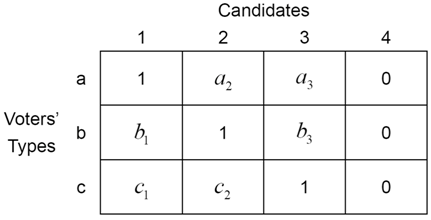
2.1. Preferences

2.2. Voting Equilibria
2.3. Electoral Systems
3. Results
3.1. Single Nontransferable Vote
3.2. Open-List Proportional Representation
3.2.1. Three-Candidate Equilibria
3.2.2. Two-Candidate Equilibria
3.2.3. Two-Pair Equilibria

3.3. Closed-List Proportional Representation
3.3.1. The Voting Stage
3.3.2. The Ranking Stage
3.4. Comparing the Three Electoral Systems
3.5. No-Tie Equilibria
4. Conclusions
Acknowledgments
Appendix
Conflicts of Interest
References
- J. Kunicova, and S. Rose-Ackerman. “Electoral Rules and Constitutional Structures as Constraints on Corruption.” Br. J. Polit. Sci. 35 (2005): 573–606. [Google Scholar] [CrossRef]
- T. Persson, and G. Tabellini. Political Economics: Explaining Economic Policy. Cambridge, MA, USA: MIT Press, 2000. [Google Scholar]
- K. Bawn, and M.F. Thies. “A Comparative Theory of Electoral Incentives: Representing the Unorganized Under PR, Plurality and Mixed-Member Electoral Systems.” J. Theor. Polit. 15 (2003): 5–32. [Google Scholar] [CrossRef]
- E. Magar, M.R. Rosenblum, and D. Samuels. “On the Absence of Centripetal Incentives in Double-Member Districts: The Case of Chile.” Compar. Polit. Stud. 31 (1998): 714–739. [Google Scholar] [CrossRef]
- B. Cain, J. Ferejohn, and M. Fiorina. The Personal Vote: Constituency Service and Electoral Independence. Cambridge, MA, USA: Harvard University Press, 1987. [Google Scholar]
- R.S. Katz. A Theory of Parties and Electoral Systems. Baltimore, MD, USA: Johns Hopkins University Press, 1980. [Google Scholar]
- R.B. Myerson, and R.J. Weber. “A Theory of Voting Equilibria.” Am. Polit. Sci. Rev. 87 (1993): 102–114. [Google Scholar] [CrossRef]
- R.B. Myerson. “Effectiveness of Electoral Systems for Reducing Government Corruption: A Game-Theoretic Analysis.” Games Econ. Behav. 5 (1993): 118–132. [Google Scholar] [CrossRef]
- R.B. Myerson. “Comparison of Scoring Rules in Poisson Voting Games.” J. Econ. Theory 103 (2002): 219–251. [Google Scholar] [CrossRef]
- G.W. Cox. “Strategic Voting Equilibria Under the Single Nontransferable Vote.” Am. Polit. Sci. Rev. 88 (1994): 608–621. [Google Scholar] [CrossRef]
- G.W. Cox, and M.S. Shugart. “Strategic Voting Under Proportional Representation.” J. Law Econ. Org. 12 (1996): 299–324. [Google Scholar] [CrossRef]
- S.R. Reed. “Structure and Behaviour: Extending Duverger’s Law to the Japanese Case.” Br. J. Polit. Sci. 20 (1990): 335–356. [Google Scholar] [CrossRef]
- E.R. Gerber, R.B. Morton, and T.A. Rietz. “Minority Representation in Multimember Districts.” Am. Polit. Sci. Rev. 92 (1998): 127–144. [Google Scholar] [CrossRef]
- T.R. Palfrey, and H. Rosenthal. “Strategic Calculus of Voting.” Public Choice 41 (1983): 7–53. [Google Scholar] [CrossRef]
- T.R. Palfrey, and H. Rosenthal. “Voter Participation and Strategic Uncertainty.” Am. Polit. Sci. Rev. 79 (1985): 62–78. [Google Scholar] [CrossRef]
- A. Schram, and J. Sonnemans. “Voter Turnout as a Participation Game: An Experimental Investigation.” Int. J. Game Theory 25 (1996): 385–406. [Google Scholar] [CrossRef]
- L. Aguiar-Conraria, and P.C. Magalhães. “How Quorum Rules Distort Referendum Outcomes: Evidence from a Pivotal Voter Model.” Eur. J. Polit. Econ. 26 (2010): 541–557. [Google Scholar] [CrossRef]
- Y. Hizen, and M. Shinmyo. “Imposing a Turnout Threshold in Referendums.” Public Choice 148 (2011): 491–503. [Google Scholar] [CrossRef]
- R.B. Myerson. “Population Uncertainty and Poisson Games.” Int. J. Game Theory 27 (1998): 375–392. [Google Scholar] [CrossRef]
- R. Shiratori. “The Introduction of a Proportional Representation System in Japan.” Elector. Stud. 3 (1984): 151–170. [Google Scholar] [CrossRef]
- M.A. Golden, and E.C.C. Chang. “Competitive Corruption: Factional Conflict and Political Malfeasance in Postwar Italian Christian Democracy.” World Polit. 53 (2001): 588–622. [Google Scholar] [CrossRef]
- 1For the classification, Kunicova and Rose-Ackerman [1] used the World Bank’s Database on Political Institutions and the index provided by Freedom House Annual Surveys. Here, “democracies” are defined as countries that achieved average scores below 5.5 in the Freedom House Annual Surveys taken during the years 1992/93 to 2000/01. This score is a measure of political freedom that takes values between 1 (most free) and 7 (least free).
- 2See Persson and Tabellini [2] for a survey of the formal analysis of why electoral systems are important (Ch. 8). They consider the effect of the ranks of candidates in a closed list, which are exogenously given, on their policy choices through their winning probabilities (Ch. 9). Bawn and Thies [3] examine a similar effect using a decision theoretic model. Magar, Rosenblum, and Samuels [4] constructed a Downsian model of open-list PR with two parties and two candidates per party to analyze which policy platform each candidate chooses. Studies on “personal vote” provide a way of distinguishing the variations of PR. Namely, electoral systems are classified into two groups in terms of whether parties have control over which of their candidates win seats (e.g., single-member district systems and closed-list PR) or not (e.g., majoritarian systems with primary elections, the single nontransferable vote, and open-list PR). Candidates’ incentives to cultivate their personal reputation among their constituencies (Cain, Ferejohn, and Fiorina [5]) and the degree of internal disunity of parties (Katz [6]) under each category of electoral system are analyzed empirically in the literature.
- 3In Myerson’s [8] voting model with corruption, the presence of another policy dimension as well as the corruption level enables corrupt parties (or candidates) to win seats under the plurality rule and the Borda rule. In our model, on the other hand, the presence of a popular candidate in the same party enables the least-preferred candidate to win a seat under PR. Myerson [9] also shows that a least-preferred candidate can win a seat under negative voting in a largePoisson game.
- 4Under cumulative voting, each voter has two votes and is allowed to cast two votes for one candidate. Under straight voting, each voter is required to split the two votes between two candidates. Under both rules, casting only one vote is also allowed. Gerber, Morton and Rietz [13] also conducted laboratory experiments to test the theoretical predictions.
- 5Suppose that one of two winners is candidate 4. All types of voters receive zero utility from the winning of candidate 4. If candidates 4 is replaced with candidate 1 in the set of winners, for example, then the utilities of types a, b, and c increase by 1, , and , respectively. Since the utilities of all types of voters increase without decreasing the utility of any type of voter, this replacement is Pareto improving. A similar calculation applies to the replacement of candidate 4 with candidates 2 and 3. Note that every outcome in which candidate 4 does not win is Pareto efficient because each of candidates 1, 2, and 3 is most preferred by one of the three types of voters.
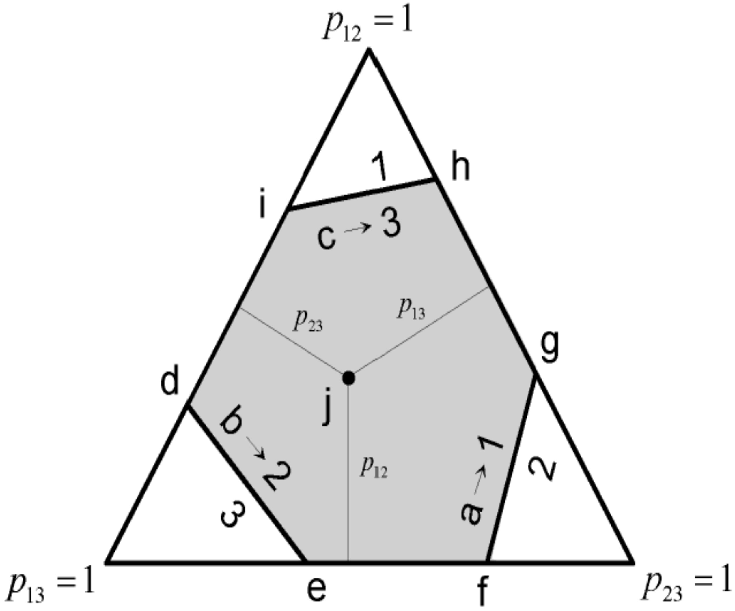
- 6In the general equilibrium model, we first derive how many units of each commodity each consumer (firm, respectively) buys (sells) according to the price vector of commodities. We then find a price vector for which the payoff-maximization behaviors of consumers and firms equate demand and supply in each market. Here, we first examine how each type of voter votes according to the vector of close-race probabilities. We then find a vector of close-race probabilitiesfor which the payoff-maximization behaviors of voters result in an electoral outcome that is consistent with theclose-race probabilities.
- 7Here, we omit the index of each voter to simplify the expressions.
- 8If close-race probabilities, which are only perceived by voters in their decisions, are replaced with pivot probabilities (i.e., actual probabilities of each vote affecting the outcome, which are calculated based on the strategies other voters choose), the objective function then becomes the exact, rather than approximate, expression of the increment of a voter’s expected utility. The pivot probability of a vote for candidate i changing the winner from candidate j to candidate i is different from the pivot probability of a vote for candidate j changing the winner from candidate i to candidate j: the former (latter, respectively) is the sum of the probability that candidate i is one vote behind (ahead) candidate j and the probability that candidates i and j obtain the same number of votes, multiplied by . Such a distinction is absent if candidates’ competitions are described with close-race probabilities.
- 9This condition requires voters to perceive that at least one close race occurs. Myerson and Weber [7] interpret such close-race probabilities as probabilities of each vote affecting the outcome conditional on the occurrence of close races for the second seat. In other words, when voters make voting decisions, they care about how their votes would affect the outcome if their votes affected the outcome. Note that only the large/small relationship between close-race probabilities matters in voting decisions.
- 10We may allow voters to perceive different close-race probabilities from each other to some extent as long as the consistency between the close-race probabilities and the electoral outcome is maintained. However, allowing differences in perception of close-race probabilities between voters enlarges the set of close-race probabilities that are consistent with each electoral outcome. It also requires us to specify, with a reasonable criterion, the extent to which the perception of close-race probabilities is allowed to differ between voters. In order to avoid such problems and simplify our model by reducing the number of possible profiles of close-race probabilities, we require the close-race probabilities to be common to all voters.
- 11The consistency between perceptions (or beliefs) and outcomes is required in most theories that assume the rationality of decision makers. In perfect Bayesian equilibria of dynamic games with incomplete information, for example, to each decision node in each information set, players assign (as a belief) a probability of themselves being on that decision node, and these probabilities must be consistent with the probabilities calculated by Bayes’ rule based on all players’ strategies that maximize their respective payoffs based on the belief.
- 12The idea of arbitrary perception of close-race probabilities in no-tie equilibria comes from the belief players hold off equilibrium paths in dynamic games with incomplete information. That is, if an information set is not reached in a perfect Bayesian equilibrium, the player who makes decisions based on this information set is allowed to assign arbitrary probabilities to each decision node in the information set as long as the sum of the probabilities is one.
- 13Ties between candidates are created in several ways. In Palfrey and Rosenthal’s [14] model with fixed voting costs, voters randomize between going to the polls and abstaining (i.e., they choose mixed strategies) as their optimal behaviors, which creates the possibility of a tie between two candidates. In Palfrey and Rosenthal’s [15] model with incomplete information about voting costs, in which voting costs are randomly determined for each voter, each voter goes to the poll if and only if his/her voting cost is sufficiently small. As a result, each voter goes to the poll with a probability between zero and one. In Schram and Sonnemans’ [16] voting environment for laboratory experiments, two candidates have the same number of supporters, and voting costs are sufficiently small. Thus, under the plurality rule, all of the voters go to the polls, and the two candidates will be in a tie. In some models of referendums (e.g., Aguiar-Conraria and Magalhães [17]; Hizen and Shinmyo [18]), a fixed number of voters are randomly assigned one of two groups (i.e., voters who want to keep the status quo and voters who want to change the current situation). In Myerson’s [19] Poisson game, the total number of voters is also a random variable. Such uncertainty about the number of voters also creates a tie between two alternatives with positive probability.
- 14For rational voters in our model, this rule is equivalent to the following rule. Each voter writes in the name of a party on his/her ballot (party vote) and he/she can also choose one candidate from the list of the party that he/she has chosen (personal vote). Party votes are converted into the allocation of seats to parties, and personal votes are used only to determine which candidates fill the seats in each party list.
- 15Another way of formulating closed-list PR is to replace and with and . We use the former because the expression is simpler.
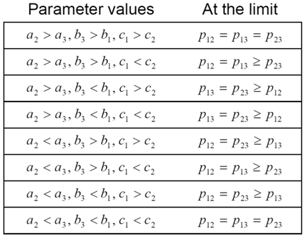
- 16For parameter values other than the first and the last rows in Table 2, one of , , and can be smaller than the other two at the limit. This indicates that the three-candidate equilibrium outcome described in Proposition 1 is relatively easy to realize in the sense that such voting behaviors are induced not only by but also by some other vectors of close-race probabilities even for extreme parameter values.
- 17If all voters abstained, then could hold. However, at least type-c voters receive a positive payoff by voting for candidate 3 and so go to the polls.
- 18As long as the three conditions are satisfied, some of the voters may vote in a different way. For example, a part of type-a (b, respectively) voters may vote for candidates 1 (2) and 4 randomly.
- 19Only if , some type-a voters may use mixed strategies among the two parties and abstention as theirpayoff-maximization behaviors because both voting for either party and abstaining result in zero payoffs for them (i.e., if ).
- 20If some type-b and type-c voters vote for the left-wing party with certainty, the left-wing party obtains more than of valid votes with certainty, and hence wins at least one seat. Then, the first-ranked candidate of the left-wing party, who is either candidate 1 or 2, wins a seat with certainty, which is inconsistent with either or .
- 21By the same logic, we also have no-tie equilibria under open-list PR in which voters perceive a sufficiently high probability of a close race between candidates 1 and 2, where the left-wing party wins two seats with certainty.
© 2015 by the authors; licensee MDPI, Basel, Switzerland. This article is an open access article distributed under the terms and conditions of the Creative Commons Attribution license (http://creativecommons.org/licenses/by/4.0/).
Share and Cite
Hizen, Y. Does a Least-Preferred Candidate Win a Seat? A Comparison of Three Electoral Systems. Economies 2015, 3, 2-36. https://doi.org/10.3390/economies3010002
Hizen Y. Does a Least-Preferred Candidate Win a Seat? A Comparison of Three Electoral Systems. Economies. 2015; 3(1):2-36. https://doi.org/10.3390/economies3010002
Chicago/Turabian StyleHizen, Yoichi. 2015. "Does a Least-Preferred Candidate Win a Seat? A Comparison of Three Electoral Systems" Economies 3, no. 1: 2-36. https://doi.org/10.3390/economies3010002
APA StyleHizen, Y. (2015). Does a Least-Preferred Candidate Win a Seat? A Comparison of Three Electoral Systems. Economies, 3(1), 2-36. https://doi.org/10.3390/economies3010002