Macroeconomic and Distributional Impacts of Jatropha Based Biodiesel in Mali

Abstract

Mali has introduced a program to produce biodiesel using jatropha, a shrub widely available throughout the country. The aim of the program is to partially substitute diesel, which is entirely supplied through imports, with domestically produced biodiesel. In this paper, we use a computable general equilibrium (CGE) model and a microsimulation model to analyze macroeconomic and distributional impact of a hypothetical expansion of jatropha based biodiesel industry in Mali. We find that the expansion of biodiesel industry (i.e., both jatropha farming and oil conversion), would increase GDP, though slightly, if idle lands are utilized for jatropha cultivation. However, the expansion of jatropha would cause slight loss in GDP if the existing agriculture land is used for jatropha cultivation. The distributional results are slightly different. We find that rural poverty would decrease no matter whether idle lands or existing agricultural lands are used for jatropha plantation, although the percentage reductions in rural poverty are higher in the former compared to the latter case. Our results indicate that if governments plan to promote jatropha biodiesel they should not allow jatropha to compete with food staples on the existing land. Policies should be targeted to utilize the idle lands which have not been used for any productive use.

1. Introduction

Some Sub-Saharan African countries, such as Mali, have expressed interest in biofuels because these countries do not have land supply constraints for producing biofuels and they are dependent on imported fossil fuels for meeting their fuel demand for transportation and electricity generation. Per capita energy consumption of Mali, in 2016, was 0.27 tons of oil equivalent (toe) of which biomass (wood, charcoal, agricultural wastes) was the predominant, 68% (ENERDATA 2018). Also, the country is strongly dependent on petroleum products imported primarily via the ports of Abidjan and Dakar. These petroleum products account for 28% of the national energy consumption (ENERDATA 2018). Biomass supplies about 78% of household energy needs and biomass burning for cooking is the main source of indoor air pollution causing high death toll of women and children (AfDB 2015). Rate of electrification is one of the lowest in Africa with only 15% of the total rural households have access to electricity (AfDB 2015). It is projected that electricity demand (peak load) would exceed 800 MW, of which half of it would be imported from neighboring countries (API 2011).

Biomass resource potential is abundant; about 33 million hectares has standing forests that can produce fuel wood and there exists enough agricultural lands with several million tons of agricultural residues and plant wastes available for energy use (AfDB 2015). Mali is one of the very few countries in the world to attempt developing biofuels, particularly from jatropha. The 2006 national energy strategy strongly stressed the need for development of biofuels, including jatropha based biodiesel. A national institution “National Agency for the Development of Biofuels (ANADEB)”1 was established in 2009 to promote biofuels in line with the 2006 national energy strategy. The 2008 National Biofuel Strategy identified two biofuels with great potential: ethanol and jatropha oil (vegetable oil as well as biodiesel). However, biofuel production in Mali did not expand the way it was anticipated in the national energy strategies for several reasons2. This happened not only in Mali but also in most countries where jatropha was seen a promising option at the beginning. The special issue of Sustainability (2014, vol. 6) has published 16 articles discussing various reasons for the failure of jatropha biofuel. Most of the articles use qualitative approach; three studies out of 16 papers published in the volume (Acheampong and Campion 2014; Portner et al. 2014; Romijn et al. 2014), present some quantitative evidence to explain the reasons. However, none of the studies conducts detailed economic analysis covering the macroeconomic and distributional impacts of jatropha based biofuels. This analysis aims to fill the research gap.

One hypothesis that helps explain the failure of jatropha biodiesel is the opportunity cost of land. Farmers are unlikely to switch over to new crops, especially perennial crops, like jatropha, which has a long life. If they want to switch over to other crops, their investments on jatropha plantation would be lost and they have lost the value of other crops that would have produced from the same land had they not used it for jatropha plantation? Moreover, there would be additional cost to convert jatropha planted land for other crops. The government did not have information of the consequences of promoting biofuels, particularly their overall economic and environmental costs and benefits. Moreover, an expansion of biofuels have wider external or indirect impacts, such as food security, waste water pollution, reduction of local air pollution, energy dependency and the fight against soil erosion. In terms of food security, the main concern is to maintain cereal production, which is the principal staple for rural Malian households (République du Mali 2008). Concerns have been raised with respect to the potential needs of land and labor to contribute to the expansion of the biofuel sectors. These factors could be taken directly from the other agricultural sectors such as cereal subsector. In this context, it is very important to carefully examine wide-reaching economy-wide and distributional impacts of expansion of biofuels before any promotional policies are designed. However, no study exists neither for Mali nor for the entire Sub-Saharan Africa. It is further important to empirically analyze the suitability of jatropha for biofuel production in Mali and similar countries in the region before governments allocate financial and institutional resources for its promotion.

In this study, we try to examine economy wide and distributional consequences of biofuels to be produced from jatropha in Mali. We selected jatropha because the Malian government planned almost for a decade to develop biodiesel from jatropha with a pre-assumption that jatropha based oil (vegetable oil as well as biodiesel) was the best feedstock to promote biodiesel in Mali as it was believed that it can be grown in marginal lands, it requires minimum input, such as fertilizer, irrigation, pesticides and it does not necessarily compete with production of food crops. But the government decision was not necessarily based on rigorous scientific and economic analysis, it was based on perception, which might have been created by the global jatropha whim about a decade ago. It is therefore important to conduct a rigorous study based on sophisticated analytical tool to understand the economics of jatropha based biodiesel not only from investors’ perspective but also from wider-economic and societal perspective. The findings of this study contribute to fill the knowledge gap. The insights derived from this study are not only helpful to Mali but also provide important guidance to policy makers in similar countries where governments want to promote jatropha based biodiesel but do not have adequate knowledge on its broader economic and distributional impacts. However, it yields more on better soils with better economic returns. Moreover, jatropha production is quite labor intensive, especially for harvesting and this will have an impact on labor markets. Although the labor-intensive harvesting increases production costs, it could provide new jobs to unskilled labor in rural areas. Thus, it is important to gain better understanding of the impacts of the expansion of jatropha production and the biofuels sector. Namely how does scaling up production affects food prices; how would increase production of biofuels affect the production of other tradable goods as well as non-tradable commodities; how would it alter the terms of trade (reduction of oil imports); how would large-scale diversion of land for biofuel production affect poverty and inequality?

The overall objective of this study is to assess the economic and distributional impact expansion of jatropha plantation and biodiesel production from it. While the economy-wide impacts are assessed using a CGE model, the distributional impacts are assessed using a micro-simulation model.

2. Methodology

2.1. The Model

Since the late 1990s, researchers have been using CGE models to analyze the impact of policy reforms on poverty and income distribution. Three main categories of these models have been used during this period: the representative household approach (RH), the integrated multi-household approach (IMH) and the micro-simulation sequential approach (MSS).

The CGE-RH approach divides households into groups, choosing a representative household for each group. The variations in income of the representative agents generated with the CGE model are applied to households within their respective group from a household survey. This assumption does not allow the analyst to take into account within-group changes in income distribution, even though studies (Huppi and Ravallion 1991; Savard 2005, for example) have shown that such changes can be greater than between-group inequality changes. Savard (2005) demonstrated that the results of poverty and income distribution analysis can be completely reversed by taking into account within-group distributional effects.

To solve this problem, a second approach, the CGE integrated multi-household approach (CGE-IMH) was proposed by Decaluwé et al. (1999) and applied by inter alia Cogneau and Robilliard (2000); Gørtz et al. (2000) and Cockburn (2001). This method incorporates a large number of households from a household survey (and sometimes all of them) into the CGE model. The approach takes into account within-group distributional effects and has the further advantage of providing coherence between the micro and macro parts of the model but at a cost. First, data reconciliation can be very problematic (Rutherford and Tarr 2007); second, numerical resolution can be challenging (Chen and Ravallion 2004).

The third approach is referred to as the CGE micro-simulation sequential method (MSS) and could be subdivided into two variants. The first, micro-accounting, was formally presented by Chen and Ravallion (2004) and has been extensively applied in recent years3. The second variant, proposed by Bourguignon et al. (2005), consists of integrating, at an individual level, rich micro behavior observed at a household level such as consumption or labor supply. This version introduces more heterogeneity between households with the application of a microeconometric model. The general idea of the MSS approach is that a CGE module feeds market and factor price changes into a micro-simulation household model. The main criticism leveled at this approach is that the micro-feedback effect is not fully taken into account; the question has been raised in two literature reviews of macro-micro modeling for poverty analysis (Hertel and Reimer 2005; Bourguignon and Spadaro 2006). However, Bourguignon and Savard (2008) found that the loss of information associated with using the MSS approach can be relatively small and policy conclusions were robust between the two approaches4. In this paper, we apply the micro-accounting version of the MSS approach5.

The last two approaches (IMH, MSS), allow for rich analysis of income distribution and poverty because they include a large number of households in the modeling exercise. It allows the modeler to apply poverty and income distribution measures and indexes following policy simulations. As already mentioned, the IMH approach is the best on a theoretical basis. However, it requires construction of a balanced sub-matrix for household accounts within a standard social accounting matrix. On the other hand, with the CGE-MSS approach, the household income and expenditure do not require balancing. This provides flexibility because the micro module is solved sequentially. This flexibility is one of the two reasons behind our choice to select the CGE-MSS approach for our analysis. The second reason behind the selection of this approach is that some households will increase their labor supply and land use thereby allowing to account for discrete changes in factor effective endowments. This type of behavior cannot be models in the IMH approach that only allows for marginal changes in factor endowments.

To capture the impact of jatropha and biofuel policies on the welfare of individual households and distributional effects, we adapt a standard model to specificities of these two sectors in the Malian economy. The presentation of the model is decomposed into the CGE module and micro simulation module.

2.2. CGE Module

The CGE component of our model (hereafter referred to as the CGE module) is based on the EXTER model of Decaluwé et al. (2001), with significant further developments, which we describe herein. The production structure is substantially modified6. We adopted a multilayered production structure as illustrated in Figure 1.

Starting at the top level, we have total production of the sector (XS), which is made up of fixed value-added shares (VA) and intermediate consumption (CII), as generally assumed in standard CGE modeling. The relationship determining the level of VA is a Cobb-Douglas production function between composite labor (LD) and total capital (KDT). Producers minimize their cost of generating VA subject to the Cobb-Douglas production function. First order conditions from this process are used to determine the optimal labor demand equations. Labor (LD) is then decomposed into skilled (LDQ) and unskilled (LDNQ) labor, with the combination of these two factors being determined by a constant elasticity of substitution (CES) function, once again through a process of cost minimization. This assumption implies that changes in the relative wages of the two types of labor will lead the producer to modify the ratio between the two types of workers, subject to constraints on substitution linked to his production capacities. The total capital (KDT) is decomposed into land (LAND) and capital (KD). The same CES function is used to link these two factors.

The capital is mobile between agricultural sub-sectors and the land is fixed. Moving on to intermediate consumptions, we significantly enrich the EXTER model by decomposing these inputs into various sub-inputs. We first have the total intermediate consumption (CII) that is decomposed into energy (CIE) and other intermediate consumptions (CI). These two sub-inputs are linked with a CES function. The CIE is further decomposed into fuels (FUEL) and electricity (ENER)7. These two inputs are linked with a CES function, therefore allowing for substitution in these inputs. The fuels are further decomposed into fossil fuels (FFUEL) and biofuels (BFUEL) with the same CES functional form8. Other intermediate consumption (CI) was modeled as fixed shares from the input/output ratios computed from the data in the SAM. Given the CES function, the market share will be gained through a reduction in price of biofuels compared to the fossil fuels. Sector-specific elasticities of substitution are used to reflect differences among sectors in determining the mix of factors in each CES function.

In the CGE module, four agents are included (government, aggregate household, firms and the rest of the world). The government draws its revenues from goods and services tax, import duties, households’ and private firms’ income taxes as well as transfers from the rest of the world. Its expenditure is made up of the consumption of public services and of transfers to other agents. The aggregate private firm draws its income from capital remuneration. It spends its income by paying taxes; making transfers to other agents and saves for investment. The rest of the world is considered as an agent in a standard fashion representing economic relations between Mali and the rest of the world including imports, exports and transfers. Finally, we modelled household behavior as a single representative household.

Our hypotheses reflect the fact that Mali is a small open economy for which world prices of imports and exports are exogenous. We posit the Armington hypothesis (Armington 1969) for import demand, whereby domestic consumers can substitute domestically produced goods with imports (imperfectly) according to an elasticity of substitution. On the export side, producers can sell the goods on the local or foreign markets; their production and use are influenced by relative prices on each market and by their respective elasticity of transformation. We used the GDP deflator as a numeraire.

Our model’s equilibrium conditions are also standard. The commodity market is balanced by an adjustment of the market price of each commodity. The labor market is perfectly segmented and balances out with an adjustment of the nominal wage on each of the respective markets (skilled and unskilled)9. It is therefore possible, for workers to move from one sector to another but not from one market to another. We use two closures for the labor markets in the simulations. In the first option, labor supply is exogenous and in the second it is endogenous. In the latter case, we use a standard wage curve as in Carneiro and Arbache (2003) where labor supply increases (decreases) with an increase (decrease) in real wages in each market10. The increase in labor can come either from the extensive margin (number of hours worked) or the intensive margin (more workers enter the market). The current account balance is exogenous and it balances out with an adjustment of the nominal exchange rate11. Finally, total investment is equal to the sum of household, firm and government savings and borrowings from the rest of the world.

2.3. The Data

The social accounting matrix (SAM) necessary for the implementation of our CGE module was constructed with data drawn from an input–output table with 18 productive sectors.12 The reference year for the SAM is 2006. The data is old but no new data was available when constructing our model. Moreover, not much structural change has occurred in Mali over the last decade. Our model covers 20 production sectors, including jatropha, biofuels, fossil fuels and other energies (mainly electricity). Jatropha and biofuels were not found in the initial SAM (Coulibaly 2009). We used information from the sectoral analysis presented in Boccanfuso et al. (2012) to disaggregate the sectors from crop agriculture and fuel sectors. The size of these sectors is relatively small in Mali but they present potential for growth. The micro-household database for 4494 households was constructed from the Enquête légère intégrée auprès des ménages (ELIM-2006) survey. The main task for constructing this database is to modify the income and expenditure structures for the households based on the nomenclature of the SAM.

2.4. Micro-Simulation Household Module

In the micro household module, we include all of the 4494 households from the survey (ELIM-2006). We have specified income and expenditure functions for the households, which are parameterized on the household-specific information found in the survey. As mentioned previously, the household module is solved sequentially. Let us now describe this sequence. We first specify an income equation that reflects the income structure for each household in the ELIM-2006 survey. The endowment of factors is exogenous. We use the factor payment variations generated by the CGE module and apply them to the factor endowments. The two wage rates are also applied to labor endowments of households13. As in the CGE module, we assume that the transfers from other agents to the households are exogenous. When increases in factors such as land is required for additional jatropha production, we computed the number of households concerned based on shares of land involved in the simulations. From there, we isolated farm households in our sample and performed random draws of households to select the ones benefiting from the growth in land under jatropha cultivation. We applied the growth in land use to these households14.

This procedure provides us with the new household-specific income. We can then move on to the expenditure side. The demand functions are derived from a utility maximization process (Cobb-Douglas utility function) and this demand equation is a function of market prices and household income. The final step in the sequential resolution of the household module consists in computing the change in welfare. Implicitly, this allows us to take into account simultaneously the income and price effects on each household’s welfare.15 As in Bourguignon and Savard (2008), we use the variation of the real income to measure the change in welfare. The household-specific value shares for consumption are computed from observed figures in ELIM-2006. These shares are then used to specify a household-specific price index that is in turn used in combination with the nominal income to obtain the change in real income.

2.5. Poverty and Distributional Analysis

After selecting our criteria for household decomposition (including rural/urban divide) we can apply any type of distributional analysis. The indexes can be applied using the reference period directly from ELIM-2006 data and then for the various simulations results. The indexes selected for our distributive analysis are the Foster, Greer and Thorbecke16 (Foster et al. 1984) P_α indexes for poverty analysis and the Gini index for inequality changes. In addition to these indexes, we applied pro-poor growth analysis with the growth incidence curves (GIC) proposed by Ravallion and Chen (2003).

3. Simulations and Results

3.1. Simulations

One of the main objective of this paper is to investigate the distributional impact of a hypothetical expansion of jatropha production and associated biofuel production from jatropha in Mali. We first look at three scenarios of increasing production of jatropha. These simulations are performed by exogenously increasing the land in the jatropha sector and capital in the biofuel sector17. We performed a fifteen fold increase in land for jatropha production going from 3000 to 45,000 hectares18. The capital in the biofuel production sector is increased exogenously by fivefold to correspond to cultivation of jatropha in the increased lands19. This set of simulations can be seen as similar in nature, though larger in scale, than the extension of the biofuel industry in line with the objectives established by the National Agency for the Development of Biofuels (Government of Mali 2008) at 23,000 hectares for 201520.

Within this first set of simulations, we perform the increase in scale with two set of assumptions. In the first case, we assume that the additional land used for cultivating jatropha comes from unused idle land (sim1a) and in the second case; the expansion of the sector is done on arable land used to produce other agricultural products (sim1b). These two extreme case scenarios provide us with upper and lower bounds for our comparative analysis. Additional capital used in the jatropha sector and biofuel sector is taken from other sectors of the economy exogenously21. For the last simulation of the first set we repeat sim1b and introduce endogenous labor supply. For this assumption, we use a standard wage curve as in Annabi (2003). In this scenario, the additional workers needed to produce jatropha can come from new labor (extra workers and/or more hours worked by active workers). However, if the scenario produces downward pressure on the real wage, we will observe an increase in unemployment.

In the next set of simulations, we consider a policy intervention to promote the biofuel sector. This policy consists in subsidizing biofuel market prices by 20%. This policy provides an additional comparative advantage to this sector compared to fossil fuels. We fund this subsidy with a 1% tax on fossil fuels22. This tax rate is assumed because in simulation 2a, a 1% tax on fossil fuel plus the 20% subsidy are revenue neutral. We use this level of tax for other simulations in this set for comparative analysis purpose but this level is no longer revenue neutral given other general equilibrium effects that are different in simulations 2b, 2c and 2d.

We compare 4 case scenarios. The first one (sim 2a) is a 20% subsidy and the 1% fossil fuel tax without an increase in land and capital in the jatropha and biofuel sectors. This allows us to isolate the impact of the tax and subsidy from other effects of the next simulations.

For the next simulation (sim 2b), we combine the tax and subsidy with a tenfold increase in land for jatropha production where the land comes from idle land. The third simulation (sim 2c) in the same as sim 2b but the land is taken from other agricultural sectors and the last one (sim 2d) in this group is sim 2c with endogenous labor supply23.

The main challenge with performing sim 1c and 2d with the endogenous labor supply is to attribute the increase in labor supply to specific households. For this procedure, we randomly draw households from a group of selected households on the basis of characteristics found in the household survey.

Table 1. Simulation descriptions.

Code	Simulations Descriptions
1a	15 x increase of land for jatropha using idle land in Mali
1b	15 x increase of land for jatropha using agriculture land
1c	15 x increase of land for jatropha using agriculture land with endogenous labour supply
2a	1% tax on fossil fuels & 20% subsidy to biofuel no exogenous increase in jatropha land
2b	1% tax on fossil fuels & 20% subsidy to biofuel & 10 x jatropha land with idle land
2c	1% tax on fossil fuels & 20% subsidy to biofuel & 10 x jatropha land with exploited land
2d	1% tax on fossil fuels & 20% subsidy to biofuel & 10 x jatropha land with endegenous labour supply

summarizes these simulations.

3.2. Results

We proceed with a brief description of our macro and a few sectoral results. As we focus our analysis on a distributional impact of these scenarios, we select some key variables that play an important role in this distributional impact analysis24.

3.2.1. Macroeconomic and Sectoral Impacts

From our results presented in

Table 2. Macro level results of the CGE model, % changes from the base case.

Variables	Definition	Sim 1a	Sim 1b	Sim 1c	Sim 2a	Sim 2b	Sim 2c	Sim 2d
Yh	Household income	0.03	−0.15	−0.16	0.07	0.07	−0.11	−0.1
w1	qualifed wage	0.16	0.05	0.04	0.06	0.33	0.22	0.17
w2	non qualifed wage	0.12	−0.07	−0.05	0.09	0.26	0.06	0.04
rr	rental rate of agricultural capital	−0.56	−0.39	−0.39	−0.53	−0.64	−0.46	−0.45
Yg	Government income	0.01	−0.14	−0.14	0.00	−0.46	−0.6	−0.6
Sg	Government savings	0.03	−0.51	−0.52	−0.01	−1.71	−2.24	−2.21
Ye	Firms’ income	−0.04	−0.21	−0.21	0.07	−0.01	−0.18	−0.18
Se	Firms’ savings	−0.08	−0.44	−0.44	0.14	−0.03	−0.38	−0.37
It	total investment	−0.03	−0.5	−0.51	0.01	−1.4	−1.87	−1.84
u	unemployment	na	NA	0.11	na	na	na	−0.23
e	real exchange rate	−0.15	−0.24	−0.25	0.04	−0.08	−0.17	−0.17

Note: rental rate of agricultural capital refers to the return to capital in uses other than jatropha.

below, the first general statement we can formulate is that the impact on macro variables is relatively small. This is not surprising as the two main sectors of interest are relatively small at the reference period. In the first set of simulations, the first simulation is the one with the weakest impact at the macro level. Hence, using idle land produces a slight positive impact on most macro variables. Both GDP and economic welfare increase under this scenario. Firms seem to be the losers since income increases for households and government while it decreases for firms because most new income generated from this growth goes to households. This stems from the fact that the jatropha sector is labor intensive. The first simulation produces a small appreciation of the real exchange rate which is expected given the substitution of fossil fuels by biofuels produced locally.

When the jatropha sector competes with other agricultural sectors for land, we observe a reduction in most macro variables with the exception of the qualified wage. These results clearly indicate the followings: (i) it would not be beneficial to grow jatropha for biofuels in Mali at the expense of existing agriculture lands; (ii) it would be more beneficial to grow existing crops if new lands were to be cultivated provided that existing crops has a market. Note that biodiesel could have better domestic and export markets compared to that of existing agriculture crops. The endogenous labor supply assumption (sim1c) does not have a strong impact when comparing results with the sim1b given the small pressure on wages. We also reiterate that the capital required by the jatropha sector will be drawn from all other sectors. Hence, competition for inputs across agricultural sectors arises in land and capital. The jatropha sector also competes for workers in simulation 1a and 1b. In simulation 1b and 1c, the impact on the real exchange rate is almost twice as strong compared to the first simulation. For simulation 1b and 1c, the reduction in land available for other agricultural sectors that in turn reduce output for these products. The reduction in supply produces an increase in market price and hence produce a better returns to capital for agricultural sectors compared to simulation 1a.

The fourth simulation (2a) is interesting as it provides positive results for most variables with the exception of the rental rate of capital in agricultural sector. It is the only simulation where we observe a depreciation of the real exchange rate. As was expected, the simulation is neutral for government since the fossil fuel tax funds the subsidy to biofuels. The impact on wages is slightly positive. Simulation 2b is interesting since it produces strongest positive effects on wages and relatively strong negative impact on rental rate of agricultural capital. When comparing the government situation, we notice a relatively strong deterioration in savings (larger deficits). This is a result of the strong expansion of the biofuel sector without other compensating revenue sources. Hence, it pushes the subsidy bill higher. This produces a reduction in public savings and consequently the total investment in the economy drops.

The relatively large gap between wage and rental rate of capital should produce stronger distributional impact compared to other simulations. When comparing simulation 2b and 2c, we observe that the competition for land produces stronger negative impact on most variables and a reduction of positive effects on others. Comparing simulations 1a and 1b, there is a positive impact on both GDP and aggregate welfare when otherwise idle land is used. This is relatively intuitive, since the idle land which has a zero opportunity cost, is now brought to the production process. Although it has some crowding out effects, such as relocation of labor from other sectors to jatropha and biodiesel sectors, those effects are relatively small compared to the positive impacts of the use of idle lands. This contrasts with 1b, illustrates the negative implications of increasing production of jatropha with competition for land. This result also reveals an interesting insight: producing jatropha in existing lands by replacing existing crops would not be beneficial in Mali. It would be more interesting to examine whether jatropha or other crops would have more favorable impacts to the Malian economy if they are grown in idle lands. It depends on several factors such international prices of biodiesel and food commodities and a single country model, used in this analysis, is not suitable to answer this particular question.

We can see a similar difference between 2b and 2c. However, both of these scenarios also include the production subsidy and fossil fuel tax that are introduced as a revenue-neutral combination in simulation 2a. Comparing 2a and 2b, we see that there are essentially identical increases in household income, GDP and welfare but the combined effect of the fiscal instruments as well as the increased availability of unused land for jatropha production significantly reduces savings and investment. In effect, the subsidy adds nothing to the real output effect of the increase idle land availability in 1b, while also worsening the overall fiscal position of the country. Conversely, if the unused land were not available, the biofuel subsidy with a revenue-neutral fossil fuel tax would have similar impacts on income and welfare.

Finally, the addition of endogenous labor supply in the model leads to an increase in unemployment in simulation 1c and a decrease in simulation 2d when the fiscal instruments are combined with land use changes. In 1c, the higher real wage from increased competition for workers, plus competition for land, raises unemployment. The biofuel subsidy reverses the negative impact on unemployment. This is because the government subsidy drives the expansion of jatropha plantation and biodiesel production proportionately higher than that in Scenario 1c. Higher expansion of this sector would mean higher demand for employment25.

Moving on to the sectoral results and recognizing once again that we have limited impacts except for the jatropha and biofuel sectors, we look first at the output/value added changes (in

Table 3. Value added results of the CGE model, % changes from the base case.

Variables	Branches	Sim 1a	Sim 1b	Sim1c	Sim2a	Sim2b	Sim2c	Sim2d
Va (value added)	crop agriculture	0.21	−0.5	−0.51	0.22	0.17	−0.54	−0.53
	rice	0.13	−0.28	−0.29	0.18	0.23	−0.18	−0.17
	export	0.14	−0.46	−0.47	0.04	0.09	−0.52	−0.51
	jatropha	1069.18	1068.76	1068.62	20.48	729.4	729.09	729.3
	coton	−0.13	−0.93	−0.93	0.13	−0.33	−1.13	−1.12
	Livestock	0.03	−0.25	−0.26	0.14	−0.05	−0.33	−0.3
	forestry	0.25	−0.44	−0.44	0.28	0.31	−0.38	−0.38
	mining	−0.09	−0.08	−0.08	−0.01	−0.09	−0.08	−0.07
	agoindustry	−0.08	−0.08	−0.09	0.01	0.01	0.01	0.02
	textile	−0.05	−0.06	−0.07	−0.01	−0.13	−0.13	−0.11
	other industries	−0.19	−0.18	−0.18	−0.01	−0.09	−0.07	−0.06
	other energy	−0.05	−0.06	−0.06	0.00	−0.09	−0.09	−0.09
	biofuel	1089.94	1089.51	1089.37	21.39	743.56	743.25	743.47
	construction	−0.8	−0.87	−0.88	−0.03	−0.84	−0.91	−0.9
	commerce	0.02	0,00	0,00	0,00	−0.03	−0.05	−0.04
	transport	−0.02	−0.01	−0.01	0,00	−0.03	−0.02	−0.02
	services	−0.64	−0.62	−0.62	−0.01	−0.39	−0.38	−0.37
	banking & finance	−0.43	−0.5	−0.5	−0.01	−0.42	−0.48	−0.47
	public services	−0.2	−0.1	−0.1	−0.05	−0.29	−0.18	−0.16
	fossil fuels	−1.36	−1.38	−1.39	−0.03	−0.89	−0.91	−0.9

). The results show an interesting contrast between Scenario 2a and rest of the scenarios. If there is only a subsidy provided to promote biodiesel, jatropha sector value added increases by 20% and biofuel sector by 21%. On the other hand, jatropha sector value added increases by 10 times if land allocated to jatropha is expanded exogenously by 15 fold. Direct investment or expansion of lands for jatropha cultivation would be more powerful if the objective of the policy is to increase production of biodiesel in Mali. However, such a policy has slight negative implications to the overall economy unless idle land is utilized for jatropha production.

Expansion of jatropha plantation would cause decrease in value added in most of the sectors because jatropha plantation would crowd out both labor and capital from most of the sectors. However, these negative impacts vary across sectors and across scenarios. For example, Scenario 1a and 2b do not cause a decrease in value added of other agricultural sectors as the land required for jatropha/biofuel expansion would be supplied through new or idle lands. There are some exceptions, however. The cotton sector exhibits a slight decrease in production. The primary reason for this reduction is the crowding out effect given the reallocation of labor from cotton sector to jatropha sector. It is also interesting to note that some of the unskilled labor currently engaged in construction and service sectors might go back to agriculture sector due to expansion of jatropha plantation.

In the second and third simulations (1b and 1c), drawing land from other sectors has a negative impact on these agricultural sectors and effects on other sectors are quite similar to simulation 1a. However, the transport and commerce sectors are not negatively affected by this scenario. In these two simulations, the two sectors most negatively affected are the fossil fuels, cotton and construction sectors. For the second set of simulations, we note that the subsidy is very inefficient in generating an increase in output for the jatropha sector and biofuel sectors, which were both increased by around 20% in simulation 2a, whereas corresponding outputs increase by more than 7 folds in other scenarios.

The price effects follow a similar trend with weak effects in general for all sectors but jatropha and biofuels. As we can see from

Table 4. Market price results of the CGE model, % changes from the base case.

Variables	Branches	Sim 1a	Sim 1b	Sim1c	Sim2a	Sim2b	Sim2c	Sim2d
Pq (market price)	crop agriculture	−0.185	0.305	0.303	−0.153	−0.27	0.22	0.227
	rice	−0.098	0.13	0.132	−0.099	−0.071	0.158	0.158
	export	0.118	0.47	0.47	0.029	0.116	0.468	0.468
	jatropha	−29.576	−29.713	−29.716	33.078	−23.328	−23.482	−23.472
	coton	−0.19	0,00	−0.005	−0.045	−0.52	−0.331	−0.325
	Livestock	−0.023	0.037	0.048	−0.059	0.023	0.083	0.07
	forestry	−0.218	0.229	0.227	−0.181	−0.218	0.228	0.235
	mining	−0.056	−0.186	−0.19	0.049	0.009	−0.122	−0.121
	agoindustry	0.088	−0.052	−0.05	0.071	0.208	0.068	0.062
	textile	0.106	−0.074	−0.066	0.075	0.141	−0.039	−0.047
	other industries	−0.101	−0.229	−0.232	0.049	−0.012	−0.14	−0.141
	other energy	0.036	−0.184	−0.186	0.076	−0.067	−0.287	−0.281
	biofuel	−3.449	−3.649	−3.652	−0.08	−2.858	−3.058	−3.055
	construction	−0.428	−0.651	−0.653	0.046	−0.447	−0.67	−0.666
	commerce	0.831	0.405	0.395	0.102	0.203	−0.219	−0.187
	transport	0.233	0.076	0.071	0.059	0.139	−0.018	−0.013
	services	0.146	−0.097	−0.101	0.068	0.042	−0.2	−0.193
	banking & finance	−0.041	−0.261	−0.267	0.058	−0.063	−0.283	−0.288
	public services	0.206	0.049	0.044	0.061	0.236	0.079	0.055
	fossil fuels	−0.275	−0.48	−0.483	0.064	−0.268	−0.472	−0.469

, the strongest impact is on jatropha sector for which we observe decreases in price between 23 to 29% for all simulations. The price of biofuel decreases in all simulations given the surge in output. However, these decreases are small considering the very high increase in supply on the market.

The strong price decreases for jatropha have a positive impact on the biofuel sector. It is also very interesting to note that the subsidy to biofuel (Scenario 2a) has a positive effect on jatropha production and price. This is explained by the fact that it is the only scenario where the policy simulation is applied to biofuel sector (i.e., consumption of biofuel is subsidized) and not uniquely to jatropha cultivation, whereas land expansion for jatropha cultivation is considered in the rest of the scenarios. The subsidy also allows for a decrease in price of biofuel in combination with a more than 20% increase in output by the sector. When we combine this simulation 2a with the increase in land for jatropha production (sim2b), we greatly reduce the demand side pressure on jatropha with the supply effect and we observe a strong decrease in the price of jatropha (−23%). It is also interesting to highlight that the market prices of other agricultural goods all increase when jatropha competes with these sectors for land and these prices decrease for most sectors when there is no competition (sim1a and sim2b). These differentiated effects will play an important role in determining the distributional impact of these simulations.

The results for changes in the rental rate of capital for the nonagricultural sectors are presented in

Table 5. Rental rate of capital results of the CGE model, % changes from the base case.

Variables	Branches	Sim 1a	Sim 1b	Sim1c	Sim2a	Sim2b	Sim2c	Sim2d
r (rental rate of capital)	mining	−0.37	−0.39	−0.4	0.02	−0.19	−0.21	−0.21
	agoindustry	0.01	−0.15	−0.15	0.09	0.39	0.22	0.22
	textile	0.08	−0.11	−0.11	0.07	0.08	−0.11	−0.1
	other industries	−0.46	−0.58	−0.58	0.07	0.07	−0.05	−0.06
	other energy	−0.01	−0.23	−0.24	0.08	−0.14	−0.36	−0.35
	biofuel	437.25	436.04	435.98	45.69	1530.65	1526.93	1527.18
	construction	−2.37	−2.78	−2.78	−0.01	−2.38	−2.78	−2.77
	commerce	1.14	0.61	0.59	0.12	0.26	−0.27	−0.22
	transport	0.35	0.31	0.31	0.05	0.34	0.3	0.3
	services	−1.94	−2.08	−2.07	0.06	−0.98	−1.12	−1.12
	banking & finance	−0.97	−1.25	−1.26	0.04	−0.77	−1.05	−1.06
	fossil fuels	−4.24	−4.42	−4.44	−0.04	−2.53	−2.71	−2.72

. Since capital is fixed, each sector has a specific rental rate of capital. As expected, the biofuel sector experiences a very strong increase in returns in all simulations since all scenarios are favorable to this sector. In the first simulation (sim1a), the fossil fuels, the construction and service sectors exhibit decreases around or above 2%.

The competition from the biofuel with fossil fuels appears in all simulations. Moreover, in all simulations, the transport sector benefits from the lower fuel prices. The subsidy (sim2a) produces a positive impact on the biofuel sector but with a much smaller impact compared to the first three simulations. The trends within each set of simulations are quite similar (with the exception of sim2a). We only observe a few qualitative differences within each set of simulations such as in the textile, commerce and other industries sectors.

We complete the section with a brief description of the market penetration of biofuel (see results in

Table 6. Market penetration of biofuel.

Market Penetration of Biofuel in % of Share
Reference	0.31
Sim 1a	3.74
Sim 1b	3.74
Sim 1c	3.73
Sim 2a	0.38
Sim 2b	2.65
Sim 2c	2.65
Sim 2d	2.65

). In the first set of simulation, the exogenous expansion of the jatropha production allows biofuel to take up just over 3.7% of market share compared to fossil fuel from an initial share of just over 0.3%. The simulation 2a which is a policy intervention without exogenous growth of the jatropha sector produces an increase in market share to 0.38%. On the other hand, the 10 fold increase in land use for jatropha production (sim 2b to 2d), allows biofuels to achieve a market share of 2.65%. One important caveat of this result is that a policy instrument such as a subsidy does not contribute much to increase the share of new energy technology (e.g., biofuels, wind, solar) in a general equilibrium setting, at least in the relatively short-term. However, the subsidy policy does not have unfavorable macroeconomic and welfare impacts. On the other hand, large scale investment or forced mandate to substantially increase share of jatropha biodiesel would have adverse impacts on the overall economy and welfare.

If we put these macro and sectoral results in the context of recent findings of the development of the jatropha sector for production of biofuel, they would tend to support the claim that the hype (as defined by Tjeuw 2017) behind the development of jatropha was certainly not justified. Most macroeconomic results exhibit at best only very slight increases while in many instances, we observe a negative impact (GDP, unemployment, etc.). Moreover, as is also reported in Tjeuw (2017), given the productivity differences obtained in arable land and idle land, we are most likely to observe the growth from jatropha production competing with other agricultural productions. Hence, it is more likely that our least positive scenarios are more likely to occur.

3.2.2. Distributional Impacts

In this section, we present and analyze poverty and income distribution changes following the different scenarios. We perform this analysis at the national level and for a rural-urban decomposition. The microsimulation module allows us to compute changes in real income for each 4494 household in the model. We present the share of households as well as average per capita expenditure for each of the two groups in

Table 7. Descriptive statistics for groups.

	Definition of households	% of Households	Means of per Capita Expenditure (Fcfa)
Urban	Farm households in urban jatropha area	31.70%	631,064.8
Rural	Non-farm households outside rural jatropha area	68.30%	225,416.79
Mali		100%	377,035.72

Source: DNSI 2006.

. We observe that 31.7% of Malian households live in urban area and 68.3% in the rural zone. The average per capita expenditure of urban households is more than double (631,064 FCFA) compared to what is observed for rural households (225,416 FCFA).

Let us begin with the poverty and inequality analysis for the reference period at the national level and for the two groups (Figure 2)26. While poverty at the national level is slightly below 40%, the rural area exhibits a poverty rate slightly higher at 42%. The poverty rate is much lower in urban zones at 14.5%. When analyzing the poverty depth (FGT1) and severity (FGT2), the indexes for rural areas are just below the national level and the urban zones have much lower levels for these two indexes. Mali is a country with relatively high level of inequality with a Gini value of 0.57 for the country. However, the decomposition analysis reveals lower inequality within the two zones at 0.53 for the urban areas and even lower in rural Mali at 0.49.

For the poverty impact analysis at the national level (see

Table 8. Variation of poverty indexes by groups27.

		Mali	UrbanMali	RuralMali
Référence	FGT0	39.7%	21.18%	42.05%
	FGT1	17.42%	7.42%	17.03%
	FGT2	9.96%	3.80%	9.14%
Sim 1a	∆% FGT0	−0.05	0.12	−0.21
	∆% FGT1	−0.14	0.46	−0.31
	∆% FGT2	−0.22	0.37	−0.38
Sim 1b	∆% FGT0	−0.05	0.29	−0.26
	∆% FGT1	−0.14	0.41	−0.31
	∆% FGT2	−0.23	0.31	−0.39
Sim 1c	∆% FGT0	−0.26	−0.44	−0.6
	∆% FGT1	−0.46	−0.33	−0.51
	∆% FGT2	−0.49	−0.25	−0.5
Sim 2a	∆% FGT0	0.1	−0.17	−0.14
	∆% FGT1	0.01	0.09	−0.01
	∆% FGT2	0.03	0.1	0.07
Sim 2b	∆% FGT0	−0.02	0.18	−0.21
	∆% FGT1	−0.17	0.37	−0.36
	∆% FGT2	−0.26	0.3	−0.42
Sim 2c	∆% FGT0	−0.05	0.29	−0.21
	∆% FGT1	−0.17	0.32	−0.36
	∆% FGT2	−0.27	0.24	−0.43
Sim 2d	∆% FGT0	−0.26	−0.44	−0.55
	∆% FGT1	−0.49	−0.42	−0.56
	∆% FGT2	−0.53	−0.32	−0.55

), we observe a decrease in poverty for all indexes and all simulations. In the first set of simulations, the one with the weakest positive impact is sim1b. Looking at poverty severity, we observe the strongest reduction for the first simulation (sim1a), while sim1c exhibits the highest reduction in poverty depth index. In the second set of simulations, the sim2a seems to be the most interesting in terms of the three poverty indexes and the subsidy using idle land (sim2b) is the second best option. The sim2c produces the weakest positive results. The positive effects are the results of increasing wages in most simulations and the decrease in price of key goods for poor households (food prices, forestry, fuel, manufactured goods). The returns to agricultural capital and land are qualitatively different between simulations and hence in some cases it will attenuate the positive effects of other variables. The two simulations with endogenous labor supply contribute to improving significantly the situation of the households benefiting from new employment or more working hours (sim1c versus sim1b and sim2d versus sim2c).

When analyzing the impact of the simulations on the two groups, we observe quite intuitive results where the rural households on an aggregate basis, benefit in all simulations for all indexes while urban households benefit in some simulations and for some indexes. In fact, the positive results observed for urban households are insignificant (standard errors are greater than the variation of the indexes). We observe significant negative impact for urban households for simulations 1a, 2a and 2b. There are no cases of significant results for changes in the headcount index (FGT0) for urban households. For rural households, all simulations produce significant results for depth and poverty indexes. However, for the headcount index, only sim1a and sim2a produce significant results.

It is interesting to note that the strongest positive effects overall for the country and for rural households is with the tax and subsidy option (sim2a). In simulations with an expansion of jatropha production, we have two opposing effects at play. On one hand, the increase in income from new production is positive but on the other hand, the increase in supply generates a decrease in prices and capital returns has a negative impact.

We present the variation of the inequalities in

Table 9. Variation of Gini index by groups.

	Mali	UrbanMali	RuralMali
Gini	0.57	0.53	0.49
∆% Gini - Sim 1a	−0.081	0.028	−0.051
∆% Gini - Sim 1b	−0.07	0.043	−0.048
∆% Gini - Sim 1c	−0.125	−0.036	−0.104
∆% Gini - Sim 2a	−0.002	0.006	−0.022
∆% Gini - Sim 2b	−0.006	0.026	0.328
∆% Gini - Sim 2c	0.005	0.041	0.33
∆% Gini - Sim 2d	−0.051	−0.037	0.275

. The sim1c is the only one that produces a reduction in inequality for the country and the two groups. Two simulations produce across the board increase in inequality (sim2c and sim2d). Other simulations (sim1a, sim1b and sim2a) generate benefits to one group and for the national level. Finally, for one simulation (sim2b), we observe a reduction of inequality at the national level but not for subgroups.

For the decomposition analysis (sub-groups), the positive results obtained for poverty in rural areas do not translate in reduction in inequality in all simulations. It is only the case for the simulations of the first set. We observe increases in inequality for all simulations in the second set for the rural area. For urban zones, the negative results for poverty translate into increase in inequality for most simulations.

In light of the claims of promoters of jatropha, that it has great potential to reduce rural poverty, our results illustrate that there is some potential for poverty reduction. However, these reductions in poverty seem relatively limited. The reduction in poverty headcount (FGT1) are between 0.1% and 0.3% with the exception of simulation 2a (−1.02%).

3.2.3. Pro-Poor Analysis

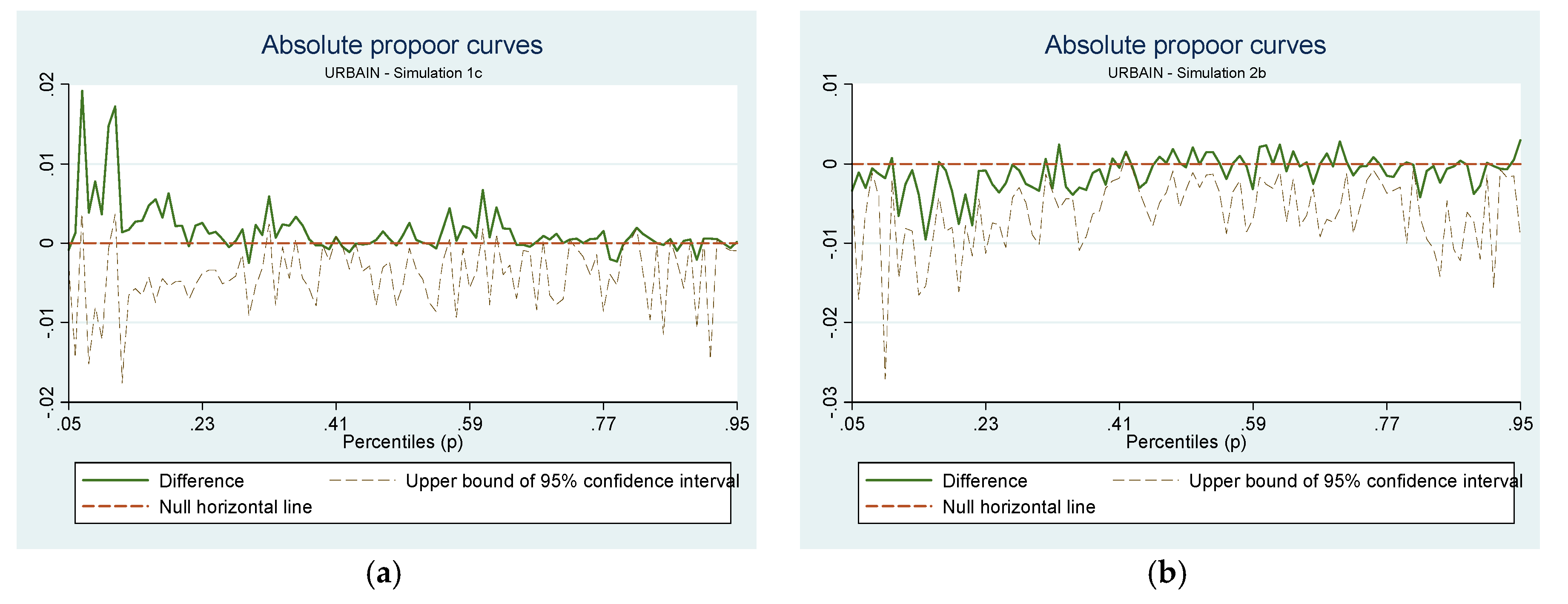
To complete our distributional impact analysis, we examined whether the simulations can be classified as pro-poor or pro-rich. To conduct this analysis, we used the growth incidence curve (GIC) developed by Ravallion and Chen (2003). This analysis allows us to see whether the variation in real income generated by the model is distributed across the distribution. The curve represents the change in real income for each percentile of the sample of households. Hence, a negatively sloped curve represents a pro-poor policy and a positively sloped curve a pro-rich scenario.

Figure 3a depicts the GIC for Mali for sim1c. The curve exhibit a slight negative slope and hence this simulation is more favorable to poorer households (below 60th percentile) compared to households above this 60th percentile. We recall that this simulation produces a reduction for the three poverty indexes and a reduction in the Gini index at the national level and for the two subgroups. In Figure 4b, the GIC curve for sim 2b reveals a proportional impact since we cannot identify a slope for the curve while poverty indexes decreases and the Gini index at that national level also decreased albeit this decrease was extremely small.

Figure 4 depicts the GIC for the rural households for simulation 1a (Figure 4a) and simulation 2a (Figure 4b). In panel a, we have a relatively horizontal curve with the exception of the two tails where the poorest are just below the 0 line and households between the 80th and 93rd percentile are the winners of this simulation. On the other hand, the simulation 2a consisting of taxing fossil fuels and subsidizing biofuel has a very slight positive slope. Interestingly, this simulation was the most efficient to reduce poverty in rural areas. The positive slope is coherent with the increase in inequality measured with the Gini index (+0.16).

The other curves presented were computed for urban households for simulations 1c and 2b. These two curves are interesting insofar as the trend observed is not consistent through the entire distribution. For sim1c (Figure 5a) we have a negative slope from the bottom of the distribution up to the 30th percentile and a flat curve to the top of the distribution. Hence, this simulation is favorable to the poorest households with little distributional impact for the richest 70% of the population in urban areas. On the other hand, the sim2b (Figure 5b) is slightly positively sloped below the 50th percentile and slightly negatively sloped above this 50th poverty line. In this case, the simulation is most favorable to the center of the distribution (between the 40th to the 70th percentile).

We complete the pro-poor analysis with a presentation of results from the Ravallion and Chen (2003); Kakwani and Son (2003) and Kakwani and Pernia (2001) indexes. Results are presented in

Table 10. Pro-poor numerical analysis.

	Pro-poor Measure	Mali	Urban	Rural
Sim 1a	Growth	+	−	+
	Ravallion and Chen (2003) - g	PPG	PRR	PRG
	Kakwani and Son (2003) - g	PRG	PRR	PPG
	Kakwani and Pernia (2001)	PRG	PPG	PPG
Sim 1b	Growth	+	+	+
	R&C (2003)	PRG	PRG	PPG
	K&S (2003)	PPG	NSPPG	PPG
	K&P (2001)	PPG	NSPPG	PPG
Sim 1c	Growth	+	+	+
	R&C (2003)	PRG	PRG	PRG
	K&S (2003)	NSPPG	NSPPG	PPG
	K&P (2001)	NSPPG	NSPPG	PPG
Sim 2a	Growth	+	+	+
	R&C (2003)	PPG	PRG	PRG
	K&S (2003)	PPG	NSPPG	PPG
	K&P (2001)	PPG	PPG	PPG
Sim 2b	Growth	+	−	+
	R&C (2003)	PRG	PRR	PRG
	K&S (2003)	NSPPG	PRR	NSPPG
	K&P (2001)	NSPPG	PPR	NSPPG
Sim 2c	Growth	+	+	+
	R&C (2003)	PRG	PRG	PRG
	K&S (2003)	NSPPG	NSPPG	PPG
	K&P (2001)	NSPPG	NSPPG	PPG
Sim 2d	Growth	+	+	+
	R&C (2003)	PRG	PRG	PRG
	K&S (2003)	NSPPG	NSPPG	PPG
	K&P (2001)	NSPPG	NSPPG	PPG

where PPG is used for pro-poor growth, PRG for pro-rich growth, PPR for pro-poor recession, PRR for pro-rich recession and PSPPG for non-strictly pro-poor growth28.

These results tend to confirm the graphical pro-poor analysis we have presented where no clear pattern can be extracted from this. The only simulation producing pro-poor growth with all indexes is simulation 2a. For the rural zone, the simulation 1b is the only one generating pro-poor growth for the three indexes and simulation 1a and 2a are the only one with at least one index to be pro-poor growth for the urban area. The Ravallion and Chen (2003) index seem to generate pro-rich growth in most scenarios. Kakwani and Pernia (2001) generate 10 occurrences of pro-poor growth which Kakwani and Son (2003) eight cases of pro-poor growth.

4. Conclusions

In this paper, we construct a CGE-microsimulation model to analyze macroeconomic as well as distributional impact of the hypothetical expansion of jatropha based biodiesel industry in Mali. We considered two types of land for jatropha plantation: (a) idle land, which is not used for agriculture purpose nor is protected as a natural forest; (b) lands which has been already used for agriculture. The study finds that the expansion of biodiesel industry (i.e., both farming and oil conversion activities), would increase GDP, though slightly, if idle lands are utilized for jatropha cultivation. However, the expansion of jatropha would cause slight loss in GDP if the existing agriculture land is used for jatropha cultivation. From the macroeconomic perspective, expansion of jatropha based biofuel industry would be beneficial to the country only if the plantation of jatropha is carried out in idle lands instead of existing agriculture lands. Given what the most recent studies found (see Tjeuw 2017 for a review on this issue), this is an unlikely scenario to occur at least as we simulated in our first scenario. Moreover, the potential of substitution of a large share of fossil fuels by biodiesel produced from jatropha is also unlikely in light of our findings. The share of biofuel in the total energy supply mix would be less than 4% in any scenario.

The distributional results are slightly different. The study finds that rural poverty would decrease no matter whether idle lands or existing agricultural lands are used for jatropha plantation, although the percentage reductions in rural poverty are higher in the former case compared to the latter. This is because jatropha plantation would provide higher returns to land and rural labor. The urban households are the losers from the expansion of jatropha based biodiesel as these households face price increases for other food staples and do not get the benefits from increase of jatropha based biodiesel outputs. At the national level, the distributional impacts are more favorable with reduction in inequality for 6 out of 8 scenarios. These results imply that a jatropha-biodiesel promotion program in Mali should be implemented along with compensating measures to protect urban poor from potential negative consequences.

Hence, based on our results, policy makers will find limited justification to support the sector based on economic efficiency criteria but if the objective is to reduce rural poverty in Mali, one could justify such a program. Two caveats should be considered in promoting the jatropha-biofuel sector. First, a promotion program should not create competition with other profitable agricultural productions (i.e., use idle land for jatropha production) and second, a promotion program should be accompanied by compensating measures to protect urban poor from potential negative consequences (increase in poverty).

This analysis can be extended for improved distributional analysis. The small size of the sector at the reference period constraints us in the size of the expansion of the sector. Converting the model into a sequential dynamic CGE model would help us introduce an incremental growth of the sector. However, performing distributional analysis with dynamic CGE model presents important challenges as one needs to determine who will benefit from the growth and depreciation of production factors. Very few authors have proposed convincing methodology to perform such an analysis. Another interesting extension of this model would be to introduce some endogeneity in the agricultural households’ behavior allowing them to switch from one crop to the other. The exogenous land endowment limits this type of behavior. This type of application will require some further investigation on the household behavior at the micro level for which we lack adequate databases.

References

- Acheampong, Emmanuel, and Benjamin Betey Campion. 2014. The Effects of Biofuel Feedstock Production on Farmers’ Livelihoods in Ghana: The case of jatropha curcas. Sustainability 6: 4587–607. [Google Scholar] [CrossRef]
- Adams, H. Adams, Jr., and Jane J. He. 1995. Sources of Income Inequality and Poverty in Rural Pakistan. Research Reports 102. Washington: International Food Policy Research Institute (IFPRI). [Google Scholar]
- African Development Bank. 2015. The Bank Group’s Strategy for The New Deal on Energy for Africa 2016–2025. Abidjan: African Development Bank. [Google Scholar]
- Annabi, Nabil. 2003. Modeling Labour Markets in CGE Models: Endogenous Labor Supply, Unions and Efficiency Wage. New York: Mimeo, Pep-net, CIRPEE, Laval University. [Google Scholar]
- API. 2011. Promotion de l’investissement privé au Mali. Opportunités pour les investisseurs dans la filière Energie. Mise à jour: Décembre 2011. Available online: https://docplayer.fr/14012912-Promotion-de-l-investissement.html (accessed on 29 May 2018).
- Armington, S. Paul. 1969. A Theory of Demand for Products Distinguished by Place of Production. IMF Staff Paper 16: 159–76. [Google Scholar] [CrossRef]
- Blanchflower, David G., and Andrew Oswald. 1998. The Wage Curve, 1st ed. Cambridge: MIT Press, vol. 1, p. 026202375. [Google Scholar]
- Boccanfuso, Dorothée, and Caroline Ménard. 2009. La croissance pro-pauvre: Un aperçu exhaustif de la boîte à outils. GREDI Working Paper No. 09-06. Sherbrooke, QC, Canada: Université de Sherbrooke. [Google Scholar]
- Boccanfuso, Dorothée, Massa Coulibaly, Luc Savard, and Govinda R. Timilsina. 2012. The Prospects of Developing Biofuels in Mali. Working Paper No. 12-03, GREDI. Sherbrooke, QC, Canada: Université de Sherbrooke. [Google Scholar]
- Boeters, Stefan, and Luc Savard. 2013. Labour Market Modelling in a CGE Context. In Handbook of Computable General Equilibrium Modeling. Edited by Peter B. Dixon and Dale Jorgenson. North-Holland: Elsevier, vol. 1B, pp. 1645–718. [Google Scholar]
- Bourguignon, François, and Luc Savard. 2008. Distributional Effects of Trade Reform: An Integrated Macro-Micro Model Applied to the Philippines. In The Impact of Macroeconomic Policies on Poverty and Income Distribution Macro-Micro Evaluation Techniques and Tools. Edited by François Bourguignon, Maurizio Bussolo and Luiz A. Pereira da Silva. London: Palgrave-Macmillan Publishers Limited, Houndmills, pp. 177–212. [Google Scholar]
- Bourguignon, François, and Amedeo Spadaro. 2006. Microsimulation as a Tool for Evaluating Redistribution Policies. Journal of Economic Inequality 4: 77–106. [Google Scholar] [CrossRef]
- Bourguignon, François, Anne-Sophie Robilliard, and Sherman Robinson. 2005. Representative versus Real Households in the Macroeconomic Modeling of Inequality. In Frontiers in Applied General Equilibrium Modeling. Edited by Timothy J. Kehoe, T. N. Srinivasan and John Whalley. Cambridge: Cambridge University Press, pp. 219–53. [Google Scholar]
- Card, David. 1995. The Wage Curve: A Review. Journal of Economic Literature 33: 785–99. [Google Scholar]
- Carneiro, Francisco Galrão, and Jorge Saba Arbache. 2003. The Impacts of Trade on the Brazilian Labor Market: A CGE Model Approac. World Development 31: 1581–95. [Google Scholar] [CrossRef]
- Chen, Shaohua, and Martin Ravallion. 2004. Welfare Impacts of China’s Accession to the World Trade Organization. World Bank Economic Review 18: 29–57. [Google Scholar] [CrossRef]
- Cockburn, John. 2001. Trade Liberalization and Poverty in Nepal: A Computable General Equilibrium Microsimulation Analysis. Working Paper 01-18, CREFA. Québec, QC, Canada: Université Laval. [Google Scholar]
- Cogneau, Denis, and Anne-Sophie Robilliard. 2000. Income Distribution, Poverty and Growth in Madagascar: Micro Simulations in a General Equilibrium Framework. IFPRI TMD Discussion Paper 61. Washington, DC, USA: International Food Policy Research Institute. [Google Scholar]
- Coulibaly, Massa. 2009. La matrice de comptabilité sociale du Mali-2006. Mimeo: GREAT-Mali. [Google Scholar]
- Decaluwé, Bernard, Jean-Christophe Dumont, and Luc Savard. 1999. How to Measure Poverty and Inequality in General Equilibrium Framework. CREFA Working Paper 9920. Québec, QC, Canada: University of Laval. [Google Scholar]
- Decaluwé, Bernard, André Martens, and Luc Savard. 2001. La politique economique du développement et les modèles d’equilibre général calculable. Montréal: Montréal University Press, pp. 1–509. [Google Scholar]
- Decaluwé, Bernar, Luc Savard, and Erik Thorbecke. 2005. General equilibrium approach for poverty analysis with an application to Cameroon. African Development Review 17: 214–38. [Google Scholar] [CrossRef]
- Direction Nationale de la Statistique et de l’information (DNSI). 2006. Enquête Légère Intégrée auprès des Ménages 2006. Bamako: DNSI. [Google Scholar]
- ENERDATA. 2018. ENERDATA Online Energy Data Base. Available online: https://estore.enerdata.net/energy-market/mali-energy-report-and-data.html (accessed on 15 May 2018).
- Foster, James, Joel Greer, and Erik Thorbecke. 1984. A Class of Decomposable Poverty Measures. Econometrica 52: 761–66. [Google Scholar] [CrossRef]
- Gørtz, Mette, Glenn Harrison, Claus Kastberg Neilsen, and Thomas Rutherford. 2000. Welfare gains of extending opening hours in Denmark. Economic Working Paper B-00-03. Columbia, SC, USA: University of South Carolina, Darla Moore School of Business. [Google Scholar]
- Government of Mali. 2008. Stratégie National pour le développement des Biocarburants au Mali; Bamako: Government of Mali.
- Hertel, Thomas, and Jeffrey Reimer. 2005. Predicting the poverty impacts of trade reform. Journal of International Trade & Economic Development 14: 377–405. [Google Scholar] [Green Version]
- Huppi, Monika, and Martin Ravallion. 1991. The Sectoral Structure of Poverty during an Adjustment Period: Evidence for Indonesia in the Mid-1980s. World Development 19: 1653–78. [Google Scholar] [CrossRef]
- Kakwani, Nanak, and Ernesto Pernia. 2001. What is Pro-Poor Growth? Asian Development Review 18: 1–16. [Google Scholar]
- Kakwani, Nanak, and Hyun H. Son. 2003. Pro-poor Growth: Concepts and Measurement with Country Case Studies. The Pakistan Development Review 42: 417–44. [Google Scholar] [CrossRef]
- King, Damien, and Sudhanshu Handa. 2003. The welfare effects of balance of payments reforms: A macro-micro simulation of the cost of rent-seeking? The Journal of Development Studies 39: 101–28. [Google Scholar] [CrossRef]
- Lachkar, Michel. 2017. Jatropha: “l’agrocarburant miracle n’a pas tenu toutes ses promesses, Géopolis Afrique. Available online: http://geopolis.francetvinfo.fr/jatropha-l-agro-carburant-miracle-n-a-pas-tenu-toutes-ses-promesses-165629 (accessed on 22 November 2017).
- Olinga Mebada, Joël Éric. 2012. Impact économique des biocarburants au Mali: Une analyse de robustesse. Sherbrooke: Mémoire de Maîtrise, Département d’économique, Université de Sherbrooke. [Google Scholar]
- Portner, Brigitte, Albrecht Ehrensperger, Zufan Nezir, Thomas Breu, and Hans Hurni. 2014. Biofuels for a Greener Economy? Insights from Jatropha Production in Northeastern Ethiopia. Sustainability 6: 6188–202. [Google Scholar] [CrossRef] [Green Version]
- Ravallion, Martin. 1994. Poverty Comparisons. Abingdon: Harwood Academic Publishers, pp. 1–143. [Google Scholar]
- Ravallion, Martin, and Shaohua Chen. 2003. Measuring Pro-Poor Growth. Economic Letters 78: 93–99. [Google Scholar] [CrossRef]
- République du Mali. 2008. Orientations stratégiques et priorités d’investissements pour un développement agricole efficient et une croissance accélérée. Bamako: Table ronde des bailleurs de fonds du Mali, pp. 1–54. [Google Scholar]
- Romijn, Henny, Sanne Heijnen, Jouke Rom Colthoff, Boris de Jong, and Janske van Eijck. 2014. Economic and Social Sustainability Performance of Jatropha Projects: Results from Field Surveys in Mozambique, Tanzania and Mali. Sustainability 6: 6203–35. [Google Scholar] [CrossRef]
- Rutherford, Thomas F., and David G. Tarr. 2007. Poverty Effects of Russia’s WTO Accession: Modeling ‘Real’ Household and Endogenous Productivity Effects. Journal of International Economics 75: 131–50. [Google Scholar] [CrossRef]
- Savard, Luc. 2005. Poverty and Inequality Analysis within a CGE Framework: A Comparative Analysis of the Representative Agent and Microsimulation Approaches. Development Policy Review 23: 313–32. [Google Scholar] [CrossRef]
- Sidibé, Abdoulaye Alfadi. 2017. Biocarburant au Mali: 740000 litres d’huile de pourghère réculté en 2016. Journal Scientifique et Technique du Mali. Available online: http://www.jstm.org/biocarburant-au-mali-740-000-litres-dhuile-de-pourghere-recoltes-en-2016/ (accessed on 22 November 2017).
- Tjeuw, Juliana. 2017. Is There Life after Hype for Jatropha? Exploring Growth and Yield in Indonesia. Ph.D. Thesis, Wageningen University, Wageningen, The Netherlands; 223p. [Google Scholar]
- Vos, Rob, and Niek De Jong. 2003. Trade liberalization and poverty in Ecuador: A CGE macro-microsimulation analysis. Economic System Research 15: 211–32. [Google Scholar] [CrossRef]