Educing AI-Thinking in Science, Technology, Engineering, Arts, and Mathematics (STEAM) Education


National Institute of Education, Nanyang Technological University Singapore, Singapore 639798, Singapore
*
Author to whom correspondence should be addressed.
Educ. Sci. 2019, 9(3), 184; https://doi.org/10.3390/educsci9030184
Submission received: 29 June 2019
/
Revised: 9 July 2019
/
Accepted: 9 July 2019
/
Published: 15 July 2019
(This article belongs to the Special Issue Trends in STEM Education)
Abstract
:In science, technology, engineering, arts, and mathematics (STEAM) education, artificial intelligence (AI) analytics are useful as educational scaffolds to educe (draw out) the students’ AI-Thinking skills in the form of AI-assisted human-centric reasoning for the development of knowledge and competencies. This paper demonstrates how STEAM learners, rather than computer scientists, can use AI to predictively simulate how concrete mixture inputs might affect the output of compressive strength under different conditions (e.g., lack of water and/or cement, or different concrete compressive strengths required for art creations). To help STEAM learners envision how AI can assist them in human-centric reasoning, two AI-based approaches will be illustrated: first, a Naïve Bayes approach for supervised machine-learning of the dataset, which assumes no direct relations between the mixture components; and second, a semi-supervised Bayesian approach to machine-learn the same dataset for possible relations between the mixture components. These AI-based approaches enable controlled experiments to be conducted in-silico, where selected parameters could be held constant, while others could be changed to simulate hypothetical “what-if” scenarios. In applying AI to think discursively, AI-Thinking can be educed from the STEAM learners, thereby improving their AI literacy, which in turn enables them to ask better questions to solve problems.
1. Introduction
1.1. The Theoretical Basis of AI-Thinking
During the usage of advanced data analytics techniques based on artificial intelligence (AI), such as machine learning, complex features that characterize the problem to be solved can be autonomously extracted without laborious human intervention. However, it does not mean that there is no role for humans to play here. Humans still need to play the leading role in the interpretation of the findings that have been generated by the AI, with the domain knowledge that humans uniquely have, based on their rich lived experiences. In the realm of understanding that straddles both AI and human-centric domains, humans will continue to play a vital role. The conceptual notion of this form of understanding and thinking—AI-Thinking—was first offered by Zeng [1] as a framework that could be used for leveraging data analytics with cognitive computing, and thereby enhance learning by challenging humans to interpret new findings from the machine-learned discovery of hidden patterns in data. The interplay of the usage of artificial intelligence and mathematics education has been observed to be capable of educing (drawing out) AI-Thinking in students [2]. Beyond the technical skills that the students could learn, science, technology, engineering, arts, and mathematics (STEAM) educators are also interested in inculcating AI-Thinking [1,3] in students, as AI has been shown to be beneficial to engaging students in STEAM education [4]. It is worthy to note that the term “arts” does not only refer to the fine arts per se; it also includes the liberal arts and the social sciences (e.g., philosophy, psychology, literature, sociology, education, etc.), in which critical thinking and rigorous human reasoning using formal logical and informal argumentations feature prominently, and hence could benefit from AI-Thinking.
In the focused context of the current paper, the term AI-Thinking could be construed as follows: “AI” represents machine-based artificial intelligence, while “thinking” represents human-in-the-loop (HuIL) [5] reasoning. STEAM practitioners must be educated, so that they would be able to recognize opportunities which AI could be applied in the domains they are interested in, where they can transform human-centric ideas into technical inputs that the AI technology can understand. When the AI technology presents technically detailed results after performing computations on the data, in order to understand and interpret the findings in meaningful human-centric terms, STEAM practitioners would have to be informed enough about the technical details of how the AI processed the data (e.g., in the present context, to be at least knowledgeable about how the mathematical algorithm of the Bayesian theorem works).
It would not be unreasonable to assume that AI-Thinking is not a linear thinking process. From a complex thinking and learning educational phenomenon perspective [6], it could be understood as the co-emergence of at least two main concomitant types of thinking reaching a state of “vital simultaneities” [7], that is, in human-initiated AI analysis on the dataset informing human-centric reasoning in terms from STEAM-related domains, and vice-versa, in STEAM-related human-centric reasoning informing further AI analysis on the dataset, and so on. They are inextricably intertwined and cannot be easily pried apart. Nevertheless, even though AI-Thinking is elusively complex and might be challenging to include as part of formal assessments in educational curricula, it behooves us to bear in mind that the importance of educing AI-Thinking in STEAM practitioners could not be overstated, as policy makers and STEAM educators embark on this adventure to train students via informal educational programs in an era where—like it or not—the use of AI is becoming more ubiquitous across industries and societies.
1.2. The Role of AI in Education
AI has always played a supporting role in contemporary education. Since the 1980s, AI has been utilized in education to assist teachers and to enhance the learning experiences of students [8,9]; albeit in small numbers around the globe. The field of artificial intelligence in education (AIED) has progressed alongside the development of pedagogical theories, practices, and goals of education [10,11,12]. Thus far, however, the focus of AIED has primarily been on empirical studies about the successful usages of computers software applications or toy-like programmable robots to teach well-defined STEM-related conceptual knowledge [10]; albeit, often without as much considerations about inclusion of the letter “A” which represents the arts. This was understandable as many curricula in the past were often crafted by separate faculties or departments, unless specially called upon for collaborations across domains. Moreover, AI has been more closely associated with the computer science departments in universities, rather than with the science, engineering, mathematics, or art departments. However, in recent years AI has gained so much traction across industries that the notion of AI-infused industries has been referred to as “Industry 4.0” [13]. This underscores the importance of training students not just in problem-solving using seminal concepts which they learn from STEAM, but also from AI.
In recent years, STEAM education has become an integral part of pre-tertiary education, reaching out to students in kindergartens, elementary schools, middle schools, and high schools. Conducting research into AI’s supporting role as educational scaffolds for students can contribute to a better understanding of how their learning processes can be enhanced [14]. Educators have been trying to introduce to pre-university students popular AI concepts such as machine vision, natural language processing (NLP), machine learning (ML), deep learning (DL), or reinforcement learning (RL), and thereafter train these students to create artificial neural networks (ANN), recurrent neural networks (RNN), convolutional neural networks (CNN), or generative adversarial networks (GAN).
Ideally, in order for students to learn about these AI-related concepts, they would need to first master a computer programming language such as C++, Python or Julia, and subsequently learn to write programs to translate algorithms from mathematical symbols into computer code. It could be assumed that educators and students in pre-university levels neither have the time nor the pre-requisite skills to learn how to write programs within the precious class timeslots.
Moreover, there is a need for educators to train students to a level in which they can work in teams, discuss STEAM concepts and engage their peers using data-driven evidence-based reasoning skills. However, Correa, Bielza, and Pamies-Teixeira [15] point out that in neural networks, the relationships existing between the nodes in a model could be likened to a black box. They are either hidden from the user or are far too complex to be easily understood by humans.
2. Research Problem and Research Questions
2.1. Research Problem
Data analytics has emerged as a professional skill that STEAM practitioners (such as scientists, computer programmers, engineers, scholars of the liberal arts, and mathematicians) are expected by potential employers to possess as part of their education, regardless of whether they were taught the skill in school. It has been recognized as an essential skill to undergraduate STEAM curriculum; not just in post-graduate engineering education [16]. In order to motivate students to develop their interest in STEAM, K-12 curriculums in many countries have already included elements of science, technology, engineering, arts, and mathematics in lessons, as part of their efforts to offer integrated STEAM education. In recent years, exposure to STEAM in K-12 education for burgeoning pre-engineering students have involved the use of specialized hardware such as Lego Mindstorms toy robots [17], or by modifying the computer code of well-known machine learning tutorial examples, such as adapting the famous movie recommendation system into myriad forms of recommendation systems in other domains [18].
It behooves STEAM educators to wonder: is there a more intuitive human reasoning-centric approach for beginner STEAM practitioners that is relatively easy-to-use, so that people who might not be so familiar with computer programming or advanced mathematics can also analyze data and interpret the results? Further, is there any user-friendly AI-based software that could be used by beginner STEAM practitioners to ask hypothetical questions to experiment with different variables in various scenarios in the computational simulations, and subsequently communicate their ideas from the results of the analyzed data with colleagues, using intuitive human-centric reasoning that could also be easily understood by people who are not STEAM practitioners (e.g., business managers)? The current paper submits that there is indeed one such approach that STEAM educators could consider using. The AI-based Bayesian network (BN) probabilistic reasoning approach [19,20,21], is particularly well-suited for assisting STEAM practitioners to explore hypothetical questions using computational modeling.
At this juncture, readers who have gotten thus far might be wondering, “That is all very well and good, but can a concrete example be provided for STEAM educators and practitioners?” “Yes indeed, in the current paper, a concrete example will be offered for your consideration.” (My sincere apologies for the pun.)
To overcome the constraints that were previously mentioned, the current paper proffers an AI-based BN probabilistic reasoning approach [19,20,21], using a user-friendly software which can be implemented in the classroom for beginner STEAM learners, all within a reasonably short timeframe of perhaps one hour. To suggest how AI-Thinking can be educed in a STEAM-related educational setting, the following will be included in the current paper.
- Science: the scientific concept of entropy will be explored by measuring it in the dataset.
- Technology: a user-friendly AI-based Bayesian network software, Bayesialab, will be used.
- Engineering: a civil engineering example will be used to explore the relationship between concrete compressive strength and the variables within the mixture.
- Arts: different concrete compressive strengths might be required by the artist for creating different kinds of art works, and the artist might also have to work with pre-existing conditions or in places where cement or water or other materials might not be abundant.
- Mathematics: the mathematical formula of the Bayesian Theorem will be explained and utilized to make predictive inferences from the data.
The major theoretical paradigms that have shaped the field of AI-Thinking are logical reasoning, probabilistic reasoning, and deep data-driven learning [22]. AI-Thinking is involved in the usage of AI as a tool for analysis, in representations of complex knowledge, and in AI-development [23]. In AI-Thinking, probabilistic reasoning in data-driven cognitive models are more intuitive for grappling with uncertainties in real world problems, as it is similar to the human thinking process [3].
In light of this, the exemplars in the current paper have been purposefully designed to provide opportunities to educe AI-Thinking in the students in terms of logical reasoning (e.g., how the scarcity of one or more of the concrete mix components might necessitate the prediction and subsequent re-adjustment of new acceptable concrete compressive strength levels), probabilistic reasoning (e.g., via the Bayesian probabilistic reasoning approach), and deep data-driven learning (e.g., discovery of hidden patterns of the relationships between the concrete mixture variables and the outcomes of the compressive strengths via supervised, and semi-supervised machine learning of the dataset).
The primary advantage of BN is that its strong probabilistic theory enables users to gain an intuitive understanding of the processes involved, and enables predictive reasoning because given observations of evidence, questions can be posed to find the posterior probability of any variable or set of variables. The current paper, however, does not purport to perform comparisons between the usage of BN and ANN in predictive models; as that has already been well-documented by Correa, Bielza, and Pamies-Teixeira [15], who observe that BN can illustrate the relationships existing between the nodes in a model, and provide more information on the relationship than ANNs, which has been likened to a black box. The benefits of BN notwithstanding, the very idea of using a BN approach could and should also be questioned by the student whose AI-Thinking is being educed. In fact, this could be one of the discussions that STEAM educators might wish to consider facilitating for their students. Nevertheless, in lieu of that fruitful discussion between STEAM educators and the students, let us return to the delineation of the BN approach at hand.
Two BN models will be illustrated in the current paper: a naive BN model, followed by a semi-supervised BN model. The naive BN model [24] is the simplest type of BN model. In the context of this paper, a naive BN model considers how much each of the individual mix components (cement, water, fineaggregate, slag, superplasticizer, age, flyash, and coarseaggregate) independently contributes to the probability of achieving different levels of concrete compressive strength, regardless of any possible correlations between them. Even though disregarding the possible correlations between the variables of the mix might seem contrived at first, naive BN has been known to perform well for predictive applications in modeling of real-world scenarios [25,26].
2.2. Research Questions
The three over-arching research questions that guide the current paper are:
Research Question 1: from descriptive analytics of the dataset, what are the relations between the inputs (mixture components) and the output (concrete compressive strength)?
Research Question 2: from predictive analytics of the dataset, what are the amounts of the inputs (mixture components) which could produce the optimal output (high-level concrete compressive strength)?
Research Question 3: under conditions of uncertainties when the supply of water and/or cement is/are scarce (at low-level), what are the probabilities of producing output of low/mid/high concrete compressive strength?
3. Methods
3.1. Rationale for Using the AI-Based Bayesian Network Approach
Among a vast constellation of tools in AI-related research, the BN approach for analyzing statistical data [27] has gained traction in research in recent years [28]. The BN approach [19,20,21] is suitable for analyzing non-parametric data, because it does not require the underlying parameters of a model to assume a normal parametric distribution [29,30,31]. The Bayesian paradigm enables STEAM practitioners to perform hypothesis testing by including prior knowledge into the analyses. Consequently, it becomes unnecessary to repeatedly perform multiple rounds of null hypothesis testing [32,33,34] when using Bayesian data analytical techniques.
Researchers in education, such as Kaplan [35], Levy [36], Mathys [37], and Muthén and Asparouhov [38], Bekele and McPherson [39], and Millán, Agosta, and Cruz [40] have also utilized the Bayesian approach, because it enables them to measure information gain, as depicted in Claude Shannon’s information theory [41], which could calculate the probabilistic amount of commonality between two data distributions even if they might not be parametric.
3.2. The Bayesian Theorem
A brief introduction to the Bayesian theorem and BN will be presented here. However, it can never do justice to the well-established corpus of BN. Readers who are interested to learn more about BN are encouraged to peruse the works of Cowell, Dawid, Lauritzen, and Spiegelhalter [42]; Jensen [43]; and Korb and Nicholson [44].
The mathematical formula (see Equation (1)) upon which BN was based, was developed and first mentioned in 1763 by the mathematician and theologian, Reverend Thomas Bayes [27].
According to Equation (1), H represents a hypothesis, and E represents a piece of evidence. P(H|E) is referred to as the conditional probability of the hypothesis H, which means the likelihood of H occurring given the condition that the evidence E is true. It is also referred to as the posterior probability, which means the probability of the hypothesis H being true after calculating how the evidence E influences the verity of the hypothesis H.
P(H) and P(E) represent the probabilities of the likelihood of the hypothesis H being true, and of the likelihood of the evidence E being true, independent of each other, and is referred to as the prior or marginal probability—P(H) and P(E), respectively. P(E|H) represents the conditional probability of the evidence E, that is, the likelihood of E being true, given the condition that the hypothesis H is true. The quotient P(E|H)/P(E) represents the support which the evidence E provides for the hypothesis H.
3.3. The Research Model
The primary goal of the current paper is to offer one of myriad possible ways that AI-Thinking (regardless of how much or how little) could be educed in beginner STEAM students. The objective of the exemplars is not to promote Bayesian Network as the ultimate AI-based tool for educing AI-Thinking, but to encourage STEAM students to think about the trustworthiness of AI-based analysis techniques in general, and hopefully, to exercise AI-Thinking in order to discuss AI and STEAM with the teachers and classmates. In other words, it is far more important to get students to raise questions and think about the possibilities in problem-solving, rather than try to achieve a so-called correct answer.
The probabilistic reasoning techniques used are based on BN. The Bayesian approach has been chosen because it is a methodology that has been used for modeling the performances in STEAM-related systems where the concept of the Markov Blanket [45], in conjunction with response surface methodology (RSM) [46,47,48,49] are utilized, as they are proven techniques for examining the optimization of the relations between the variables of theoretical constructs, even if they are not physically related.
The current paper proffers an approach which enables STEAM educators to facilitate discussions pertaining to AI and STEAM with the use of descriptive analytics, as well as predictive simulations using the data that has been generously donated by Yeh [50,51,52,53,54,55] and made publicly available at the website (https://archive.ics.uci.edu/ml/datasets/Concrete+Compressive+Strength).
In subsequent sections, the detailed BN models of the knowledge about concrete mixture variables and the outcome of the concrete compressive strength will be presented. The current paper proposes a practical Bayesian approach to demonstrate how STEAM educators and practitioners—rather than computer scientists—could analyze and explore any possible hidden motif in the data, using the following two types of analytics, which will be perform first for the supervised machine learning BN model, and subsequently for the semi-supervised machine learning BN model:
- Descriptive Analytics of “What Has Already Happened?” in Section 4:
- Purpose: to use descriptive analytics to discover the motifs in the collected data.For descriptive analytics, BN modeling will utilize the parameter estimation algorithm to automatically detect the data distribution of each column in the dataset. Further descriptive statistical techniques will be employed to understand more about the current baseline conditions of the concrete mixture variables and the corresponding compressive strengths. These techniques include the use of curves analysis and the Pearson correlation analysis.
- Predictive Analytics Using “What-If?” Hypothetical Scenarios in Section 5:
- Purpose: to use predictive analytics to perform in-silico experiments with fully controllable parameters in the concrete mixture variables for the prediction of counterfactual outcomes in the concrete compressive strengths. A probabilistic Bayesian approach will be used to simulate various scenarios where constraints might exist (e.g., scarcity of water and/or cement) to better inform STEAM practitioners about how different combinations of the concrete mixture could produce different levels of concrete compressive strengths. For predictive analytics, counterfactual simulations will be employed to explore the motif of the data. The predictive performance of the BN model will be evaluated using tools that include the gains curve, the lift curve, the receiver operating characteristic (ROC) curve, as well as by statistical bootstrapping of the data inside each column of the dataset (which is also the data distribution in each node of the BN model) by 100,000 times, in order to generate a larger dataset to measure its precision, reliability, Gini index, lift index, calibration index, the binary log-loss, the correlation coefficient R, the coefficient of determination R2, root mean square error (RSME), and normalized root mean square error (NRSME).
4. Preparation of Data Prior to Machine Learning
This section presents the procedures taken in descriptive analytics to make sense of “what has already happened?” in the collected dataset. The purpose of importing the dataset comprising 1030 rows of concrete mixture components and the corresponding outcomes in concrete compressive strengths into Bayesialab, is to discover the “informational motif” [56] of the data.
4.1. Dataset of the Concrete Mixture Variables and Their Corresponding Concrete Compressive Strengths
The files of the dataset can be downloaded from the UCI Machine Learning Repository website (https://archive.ics.uci.edu/ml/datasets/Concrete+Compressive+Strength).
4.2. Codebook of the Dataset
The dataset was generously donated to the public domain by Yeh [50,51,52,53,54,55], who has produced seminal research studies to analyze concrete mix data using artificial neural networks (ANN). The current paper does not seek to belabor the laudable predictive engineering research studies which were based on ANN; rather, it hopes to offer a complementary alternative for STEAM educators to ease students into using a multidisciplinary integrative approach to engage in predictive probabilistic reasoning, AI-Thinking, and STEAM learning. The codebook of the dataset is presented in Table 1.
4.3. Software Used: Bayesialab
The software which will be utilized is Bayesialab version 8.0. The 30-day trial version can be downloaded from the website (http://www.bayesialab.com).
Before proceeding with the following exemplars illustrated in the following sections, a highly recommended pre-requisite activity which would be greatly beneficial to the reader is, to become familiar with Bayesialab by downloading and reading the free-of-charge user-guide [57] from the website (http://www.bayesia.com/book/) as it contains the descriptions of the myriad tools and functionalities within the Bayesialab software, which are too lengthy to include in the current paper.
4.4. Pre-Processing: Checking for Missing Values or Errors in the Data
Before using Bayesialab to construct the BN, the first step is to check the data (using the file “Concrete_Data_Yeh.csv”) for any anomalies or missing values. In the dataset used in this study, there were no anomalies or missing values. However, should other researchers encounter missing values in their datasets; rather than discarding the row of data with a missing value, the researchers could use Bayesialab to predict and fill in those missing values. Bayesialab would be able to perform this by machine-learning the overall structural characteristics of that entire dataset being studied using structural EM algorithms and dynamic imputation algorithms, before producing the predicted values [58].
The dataset in delimited text format (see Figure 1) was imported into Bayesialab, in preparation for machine learning analysis.
As the dataset was being imported into Bayesialab (see Figure 2), it automatically tried to categorize the data columns as “continuous” (in blue). There were no “discrete” data in this dataset.
As part of the data import process, Bayesialab could inspect the dataset (see Figure 3) to double-check it for any missing values or errors (there were none).
Discretization of the continuous data in multiple columns could be automatically performed by the Bayesialab software. The algorithm R2-GenOpt* used in this example (see Figure 4) was the optimal approach recommended by Bayesialab. It was a genetic discretization algorithm for maximizing the coefficient of determination R2 between the discretized variable and its corresponding continuous variable [59].
After the data import process was completed, unlinked nodes (see Figure 5) were presented. Each node contained data from a column of the dataset. The next section will present how machine learning was performed on the imported dataset.
5. Overview of the BN Approach Used to Machine-Learn the Data
Before presenting the results from the machine learning process performed by the BN software, a brief overview of the nomenclature used to describe the structure of the BN is presented here. Nodes (both the blue round dots, as well as the round cornered rectangles showing the data distribution histograms) represent variables of interest, for example, the input variables such as cement, blast furnace slag, fly ash, water, superplasticizer, coarse aggregate, fine aggregate, and age, in terms of kilogramme in one cubic meter (Kg in one m3) volume of the concrete mixture, and the output variable, concrete compressive strength. Such nodes can correspond to symbolic/categorical variables, numerical variables with discrete values, or discretized continuous variables. Even though BN can handle continuous variables, we exclusively discuss BN with discrete nodes in the current paper, as it is more relevant to heuristically categorize the concrete mixture input variables into high, mid, and low amounts, so that STEAM educator can easily facilitate the discussions among the students, and with the students within the short times pan of one class period (about 1 h).
Directed links (the arrows) could represent informational (statistical) or causal dependencies among the variables. The directions are used to define kinship relations, i.e., parent-child relationships. For example, in a Bayesian network with a link from X to Y, X is the parent node of Y, and Y is the child node. In the current paper, it is important to note that the Bayesian network presented is the machine-learned result of probabilistic structural equation modeling (PSEM); it is not a causal model diagram, and for this reason, the arrows do not represent causation; they merely represent probabilistic structural relationships between the parent node and the child nodes.
BN, also referred to as belief networks, causal probabilistic networks, and probabilistic influence diagrams are graphical models which consist of nodes (variables) and arcs or arrows. Each node contains the data distribution of the respective variable. The arcs or arrows between the nodes represent the probabilities of correlations between the variables [60].
Using BN, it becomes possible to use descriptive analytics to analyze the relations between the nodes (variables) and the manner (the motif or pattern) in which initial probabilities, such as the proportions of the various concrete mixture input variables (e.g., different amounts of cement, blast furnace slag, fly ash, water, superplasticizer, coarse aggregate, fine aggregate, and age), might influence the probabilities of future outcomes in the concrete compressive strengths.
Further, BN can also be used to perform counterfactual speculations about the initial states of the data distribution in the nodes (variables), given the final outcome. In the context of the current paper, exemplars will be presented in the predictive analytics segments to illustrate how counterfactual simulations can be implemented using BN. For example, if we wish to find out the conditions of the initial states in the nodes (variables) which would lead to a high probability of attaining high-level concrete compressive strength, or if we wish to find out how low inputs of cement and/or water could influence the outcome of the concrete compressive strength, we can simulate these hypothetical scenarios in the BN.
The relation between each pair of connected nodes (variables) is determined by their respective conditional probability table (CPT), which represents the probabilities of correlations between the data distributions of the parent node and the child node [61]. In the current paper, the values in the CPT are automatically machine-learned by Bayesialab according to the data distribution of each column/variable/node in the dataset. Nevertheless, it is possible but optional for the user to manually enter the probability values into the CPT, if the human user wishes to override the machine learning software. In Bayesialab, the CPT of any node can be seen by double-clicking on it.
6. Supervised Machine Learning Using the Naïve Bayes Approach
In this section, supervised machine learning via a naive Bayes model is utilized to analyze how input variables of the mixture could influence the output of concrete compressive strength.
First, descriptive analytics is performed on the collected data to learn more about the characteristics of its collective pattern or motif. Subsequently, predictive analytics using supervised machine learning will make use of the motif machine-learned in this section to generate simulations of hypothetical scenarios in-silico to forecast conditions which we might like to achieve or avoid.
6.1. “What Had Happened?” Descriptive Analytics Using Supervised Machine Learning with Naive Bayes Approach
The results of the descriptive analysis (see Figure 6) are presented as follows.
For exploration purposes, and for facilitating the ease of quick discussions about STEAM-related concepts among the students, the machine learning procedure inside Bayesialab was used to cluster the data within each component of the mixture into three levels to represent the high, mid, and low categories.
Descriptive analytics of the entire dataset revealed that, collectively from all the attempts in using different combinations of the components in the mix:
- For the node concrete compressive strength (csMPa), there was 35.15% probability of achieving low compressive strength of <=28.02 MPa (where MegaPasal is the SI unit for pressure); there was 43.11% probability of achieving mid compressive strength of >28.02 and <=48.79 MPa; and there was 21.75% of achieving high compressive strength of >48.79 MPa.
Descriptive analytics of the entire dataset revealed that, collectively from all the attempts in using different combinations of the components in the mix:
- For the attribute cement, 41.17% of the combinations in the collected data used low-level amounts of concrete in the mix (<=239.6 kg in a meter-cube mixture); 37.18% of the combinations in the collected data used mid-level amounts of concrete in the mix (>239.6 but <=362.6 kg in a meter-cube mixture); and 21.65% of the combinations in the collected data used high-level amounts of concrete in the mix (>362.6 kg in a meter-cube mixture).
- For the attribute superplasticizer, 42.52% of the combinations in the collected data used low-level amounts of superplasticizer in the mix (<=4.6 kg in a meter-cube mixture); 51.17% of the combinations in the collected data used mid-level amounts of superplasticizer in the mix (>4.6 but <=14.3 kg in a meter-cube mixture); and 6.31% of the combinations in the collected data used high-level amounts of superplasticizer in the mix (>14.3 kg in a meter-cube mixture).
- For the attribute slag, 56.41% of the combinations in the collected data used low-level amounts of slag in the mix (<=54.6 kg in a meter-cube mixture); 24.76% of the combinations in the collected data used mid-level amounts of slag in the mix (>54.6 but <=167 kg in a meter-cube mixture); and 18.83% of the combinations in the collected data used high-level amounts of slag in the mix (>167 kg in a meter-cube mixture).
- For the attribute flyash, 56.41% of the combinations in the collected data used low-level amounts of flyash in the mix (<=24.5 kg in a meter-cube mixture); 31.36% of the combinations in the collected data used mid-level amounts of flyash in the mix (>24.5 but <=134 kg in a meter-cube mixture); and 12.23% of the combinations in the collected data used high-level amounts of flyash in the mix (>134 kg in a meter-cube mixture).
- For the attribute coarseaggregate, 19.51% of the combinations in the collected data used low-level amounts of superplasticizer in the mix (<=910 kg in a meter-cube mixture); 51.75% of the combinations in the collected data used mid-level amounts of superplasticizer in the mix (>910 but <=1014.3 kg in a meter-cube mixture); and 28.74% of the combinations in the collected data used high-level amounts of superplasticizer in the mix (>1014.3 kg in a meter-cube mixture).
- For the attribute age, 81.55% of the combinations in the collected data had utilized low-level amounts of age in the mix (<=56 days); 15.24% of the combinations in the collected data had utilized mid-level amounts of age in the mix (>56 but <=180 days); and 3.20% of the combinations in the collected data used high-level amounts of age in the mix (>180 days).
- For the attribute fineaggregate, 23.20% of the combinations in the collected data used low-level amounts of fineaggregate in the mix (<=717.8 kg in a meter-cube mixture); 53.11% of the combinations in the collected data used mid-level amounts of fineaggregate in the mix (>717.8 but <=825.5 kg in a meter-cube mixture); and 23.79% of the combinations in the collected data used high-level amounts of fineaggregate in the mix (>825.5 kg in a meter-cube mixture).
- For the attribute water, 34.08% of the combinations in the collected data used low-level amounts of water in the mix (<=173.5 kg in a meter-cube mixture); 57.48% of the combinations in the collected data used mid-level amounts of water in the mix (>173.5 but <=206 kg in a meter-cube mixture); and 8.45% of the combinations in the collected data used high-level amounts of water in the mix (>206 kg in a meter-cube mixture).
6.2. “What Has Happened?” Descriptive Analytics Using Pearson Correlation Analysis
To complement the work of colleagues who might prefer to visualize data in terms of frequentist statistics, descriptive analytics can also be performed by using the Pearson correlation analysis tool in Bayesialab. In conjunction with the naive Bayes model, it can be used for initial exploration of the relations between the variables of the concrete mixture. The visualizations of the Pearson correlations can be presented so that it is easier to see the positive correlations highlighted in thicker blue lines (see Figure 7), and negative correlations highlighted in red (see Figure 8). One suggestion for the interpretation of the positive Pearson correlations could be, that the thicker blue lines and their corresponding nodes might represent the regions which could potentially impact the outcome of the concrete compressive strengths positively. The tool can be activated in Bayesialab via these steps on the menu bar: analysis > visual > overall > arc > Pearson correlation > R+ (positive correlations).
The tabular view (see Table 2) of the Pearson correlation tool can be activated in Bayesialab via these steps on the menu bar: analysis > report > relationship.
6.3. “What-If?” Predictive Analytics Using the Naïve Bayes Approach
Hypothetical Scenario 6.3.1:what amounts should be used in the component attributes in the mix if we wish to achieve high concrete compressive strength?
The results of the predictive analysis (see Figure 9) are presented as follows.
To simulate the conditions for achieving high concrete compressive strength, we set hard evidence by setting the counterfactual value of 100% on high compressive strength (>48.79 MPa) in the node csMPa, by double-clicking on it in Bayesialab. The corresponding counterfactual results of the conditions needed to achieve high concrete compressive strength are as follows:
- For the attribute cement, the probability of achieving high concrete compressive strength would be 13.39% if the low-level amount of concrete was used in the mixture (<=239.6 kg in a meter-cube mixture); the probability of achieving high concrete compressive strength would be 38.84% if the mid-level amount of concrete was used in the mix (>239.6 but <=362.6 kg in a meter-cube mixture); and the probability of achieving high concrete compressive strength would be 47.77% if the high-level amount of concrete in the mix was used in the mix (>362.6 kg in a meter-cube mixture).
- For the attribute superplasticizer, the probability of achieving high concrete compressive strength would be 22.77% if the low-level amount of superplasticizer was used in the mixture (<=4.6 kg in a meter-cube mixture); the probability of achieving high concrete compressive strength would be 62.05% if the mid-level amount of superplasticizer was used in the mixture (>4.6 but <=14.3 kg in a meter-cube mixture); and the probability of achieving high concrete compressive strength would be 15.18% if the high-level amount of superplasticizer was used in the mixture (>14.3 kg in a meter-cube mixture).
- For the attribute slag, the probability of achieving high concrete compressive strength would be 42.86% if the low-level amount of slag was used in the mixture (<=54.6 kg in a meter-cube mixture); the probability of achieving high concrete compressive strength would be 32.59% if the mid-level amount of slag was used in the mixture (>54.6 but <=167 kg in a meter-cube mixture); and the probability of achieving high concrete compressive strength would be 24.55% if the high-level amount of slag was used in the mixture (>167 kg in a meter-cube mixture).
- For the attribute flyash, the probability of achieving high concrete compressive strength would be 66.96% if the low-level amount of flyash was used in the mixture (<=24.5 kg in a meter-cube mixture); the probability of achieving high concrete compressive strength would be 25.45% if the mid-level amount of flyash was used in the mixture (>24.5 but <=134 kg in a meter-cube mixture); and the probability of achieving high concrete compressive strength would be 7.59% if the high-level amount of flyash was used in the mixture (>134 kg in a meter-cube mixture).
- For the attribute coarseaggregate, the probability of achieving high concrete compressive strength would be 28.12% if the low-level amount of coarseaggregate was used in the mixture (<=910 kg in a meter-cube mixture); the probability of achieving high concrete compressive strength would be 48.21% if the mid-level amount of coarseaggregate was used in the mixture (>910 but <=1014.3 kg in a meter-cube mixture); and the probability of achieving high concrete compressive strength would be 23.66% if the high-level amount of coarseaggregate was used in the mixture (>1014.3 kg in a meter-cube mixture).
- For the attribute age, the probability of achieving high concrete compressive strength would be 66.52% if the low-level amount of age had been utilized in the mixture (<=56 days); the probability of achieving high concrete compressive strength would be 27.68% if the mid-level amount of age had been utilised in the mix (>56 but <=180 days); and the probability of achieving high concrete compressive strength would be 5.80% if the high-level amount of age had been utilised in the mix (>180 days).
- For the attribute fineaggregate, the probability of achieving high concrete compressive strength would be 32.59% if the low-level amount of fineaggregate was used in the mix (<=717.8 kg in a meter-cube mixture); the probability of achieving high concrete compressive strength would be 45.98% if the mid-level amount of fineaggregate was used in the mix (>717.8 but <=825.5 kg in a meter-cube mixture); and the probability of achieving high concrete compressive strength would be 21.43% if the high-level amount of fineaggregate was used in the mix (>825.6 kg in a meter-cube mixture).
- For the attribute water, the probability of achieving high concrete compressive strength would be 63.84% if the low-level amount of water was used in the mix (<=173.5 kg in a meter-cube mixture); the probability of achieving high concrete compressive strength would be 28.12% if the mid-level amount of water was used in the mix (>173.5 but <=206 kg in a meter-cube mixture); and the probability of achieving high concrete compressive strength would be 8.04% if the high-level amount of water was used in the mix (>206 kg in a meter-cube mixture).
Hypothetical Scenario 6.3.2:what would happen to the concrete compressive strength if low-levels in all components of the mixture were used?
The results of the predictive analysis (see Figure 10) are presented as follows.
If the counterfactual low-levels of each component was applied in the computational model, there would be 31.83% probability of achieving low concrete compressive strength (<=28.02 MPa); there would be 52.16% probability of achieving mid concrete compressive strength (>28.02 MPa but <=48.79 MPa); there would be 16.01% probability of achieving high concrete compressive strength (>48.79 MPa).
Hypothetical Scenario 6.3.3:what would happen to the concrete compressive strength if a low-level of the amount of water was used, with the rest of the components held constant?
The results of the predictive analysis (see Figure 11) are presented as follows.
If the low-level of the amount of water was applied in the computational model, with the rest of the components in the mixture held constant in accordance with the original dataset, there would be 24.73% probability of achieving low concrete compressive strength (<=28.02 MPa); there would be 41.15% probability of achieving mid concrete compressive strength (>28.02 MPa but <=48.79 MPa); there would be 34.12% probability of achieving high concrete compressive strength (>48.79 MPa).
Hypothetical Scenario 6.3.4:what would happen to the concrete compressive strength if low-level of the amount of cement was used, with the rest of the components held constant?
The results of the predictive analysis (see Figure 12) are presented as follows.
If the low-level of the amount of cement was used, with the rest of the components held constant in accordance with the original dataset, there would be 46.55% probability of achieving low concrete compressive strength (<=28.02 MPa); there would be 43.95% probability of achieving mid concrete compressive strength (>28.02 MPa but <=48.79 MPa); there would be 9.51% probability of achieving high concrete compressive strength (>48.79 MPa).
Hypothetical Scenario 6.3.5:what would happen to the concrete compressive strength if low-levels of the amount of cement and water were used, with the rest of the components held constant?
The results of the predictive analysis (see Figure 13) are presented as follows.
If low-levels of the amount of cement and water were used, with the rest of the components held constant in accordance with the original dataset, there would be 36.13% probability of achieving low concrete compressive strength (<=28.02 MPa); there would be 46.66% probability of achieving mid concrete compressive strength (>28.02 MPa but <=48.79 MPa); there would be 17.21% probability of achieving high concrete compressive strength (>48.79 MPa).
7. Semi-Supervised Machine Learning Approach
Semi-supervised machine learning can be used to analyze the dataset and generated possible relationships between the components in the mixture. This is the main difference from the supervised machine learning method used earlier in Section 6.
7.1. Descriptive Analytics Using the Semi-Supervised Bayesian Network Machine Learning Approach
In this section, descriptive analytics can be performed on the collected data to learn more about the characteristics of its collective pattern or motif (see Figure 14). Subsequently, predictive analytics using semi-supervised machine learning will be used to reveal the motif machine-learned in this section to generate simulations of hypothetical scenarios in-silico to forecast conditions which we might like to achieve or avoid.
For exploration purposes in this paper, the machine learning procedure inside Bayesialab was used to cluster the data within each component of the mixture into three levels to represent the high, mid, and low categories.
Descriptive analytics of the entire dataset revealed that, collectively from all the attempts in using different combinations of the components in the mix:
- For the node (csMPa) concrete compressive strength, there was 35.15% probability of achieving low compressive strength of <=28.02 MPa (where MegaPasal is the SI unit for pressure); there was 43.11% probability of achieving mid compressive strength of >28.02 and <=48.79 MPa; and there was 21.75% of achieving high compressive strength of >48.79 MPa.
Descriptive analytics of the entire dataset revealed that, collectively from all the attempts in using different combinations of the components in the mixture:
- For the attribute cement, 41.17% of the combinations in the collected data used the low-level amounts of concrete in the mix (<=239.6 kg in a meter-cube mixture); 37.18% of the combinations in the collected data used the mid-level amounts of concrete in the mix (>239.6 but <=362.6 kg in a meter-cube mixture); and 21.65% of the combinations in the collected data used the high-level amounts of concrete in the mix (>362.6 kg in a meter-cube mixture).
- For the attribute superplasticizer, 42.52% of the combinations in the collected data used the low-level amounts of superplasticizer in the mix (<=4.6 kg in a meter-cube mixture); 51.17% of the combinations in the collected data used the mid-level amounts of superplasticizer in the mix (>4.6 but <=14.3 kg in a meter-cube mixture); and 6.31% of the combinations in the collected data used the high-level amounts of superplasticizer in the mix (>14.3 kg in a meter-cube mixture).
- For the attribute slag, 56.41% of the combinations in the collected data used the low-level amounts of slag in the mix (<=54.6 kg in a meter-cube mixture); 24.76% of the combinations in the collected data used the mid-level amounts of slag in the mix (>54.6 but <=167 kg in a meter-cube mixture); and 18.83% of the combinations in the collected data used the high-level amounts of slag in the mix (>167 kg in a meter-cube mixture).
- For the attribute flyash, 56.41% of the combinations in the collected data used the low-level amounts of flyash in the mix (<=24.5 kg in a meter-cube mixture); 31.36% of the combinations in the collected data used the mid-level amounts of flyash in the mix (>24.5 but <=134 kg in a meter-cube mixture); and 12.23% of the combinations in the collected data used the high-level amounts of flyash in the mix (>134 kg in a meter-cube mixture).
- For the attribute coarseaggregate, 19.51% of the combinations in the collected data used low-level amounts of superplasticizer in the mix (<=910 kg in a meter-cube mixture); 52.16% of the combinations in the collected data used the mid-level amounts of superplasticizer in the mix (>910 but <=1014.3 kg in a meter-cube mixture); and 28.32% of the combinations in the collected data used the high-level amounts of superplasticizer in the mix (>1014.3 kg in a meter-cube mixture).
- For the attribute age, 79.75% of the combinations in the collected data had utilised the low-level amounts of age in the mix (<=56 days); 16.04% of the combinations in the collected data had utilised the mid-level amounts of age in the mix (>56 but <=180 days); and 4.21% of the combinations in the collected data used the high-level amounts of age in the mix (>180 days).
- For the attribute fineaggregate, 23.56% of the combinations in the collected data had used the low-level amounts of fineaggregate in the mix (<=717.8 kg in a meter-cube mixture); 53.53% of the combinations in the collected data used the mid-level amounts of fineaggregate in the mix (>717.8 but <=825.5 kg in a meter-cube mixture); and 22.91% of the combinations in the collected data used the high-level amounts of fineaggregate in the mix (>825.5 kg in a meter-cube mixture).
- For the attribute water, 33.89% of the combinations in the collected data had used the low-level amounts of water in the mix (<=173.5 kg in a meter-cube mixture); 56.03% of the combinations in the collected data used the mid-level amounts of water in the mix (>173.5 but <=206 kg in a meter-cube mixture); and 10.08% of the combinations in the collected data used the high-level amounts of water in the mix (>206 kg in a meter-cube mixture).
7.2. Descriptive Analytics of the Semi-Supervised BN Model Using Pearson Correlations
To complement the work of colleagues who might prefer to visualize data of this semi-supervised BN machine-learned model in terms of frequentist statistics, descriptive analytics can also be performed by using the Pearson correlation analysis tool in Bayesialab. It can be used to provide another perspective of looking at the data, just in case the previous BN model (see Figure 7) missed out something due to its exploratory intent, because the relations between the mixture variables were not considered in that model. The visualizations of the Pearson correlations can be presented so that it is easier to see the positive correlations highlighted in thicker blue lines and negative correlations highlighted in red.
One suggestion for interpretation of the positive Pearson correlations (see Figure 15) could be, that the thicker blue lines and their corresponding nodes might represent the variables which could potentially impact the student positively. The tool can be activated in Bayesialab via these steps on the menu bar: analysis > visual > overall > arc > Pearson correlation > R+ (positive correlations).
One suggestion for interpretation of the negative Pearson correlations (see Figure 16) could be, that the red lines and nodes might represent the mixture variables that could potentially impact the outcome of the concrete compressive strengths negatively. The tool can be activated in Bayesialab via these steps on the menu bar: analysis > visual > overall > arc > Pearson correlation > R- (negative correlations).
The tabular view (see Table 3) of the Pearson correlation tool can be activated in Bayesialab via these steps on the menu bar: analysis > report > relationship.
7.3. Descriptive Analytics: Mapping of Entropy in the Semi-Supervised BN Model
When the ingredients of a concrete mixture physically interact with one another, it would not be unreasonable to assume that energy is involved, and that not all that energy would be converted directly into the outcomes that STEAM practitioners might wish to achieve. Clausius [62] asserts that when work is done (energy expended) on a particular entity inside a system to transform it from one state to another, not all of that energy would be converted and used to change the state of that entity. Some amount of that energy would be “spread out” into other parts of the system. Clausius refers to this “spread” of energy as entropy. This section proffers a Bayesian approach by which the notion of entropy could be visualized and analytically harnessed [63], and therefore could be used to as an area of discussion between the STEAM educator and students.
The entropy of the data distribution within each node of the BN can be visualized in Bayesialab (in validation mode) by right-clicking on each node and selecting “Display Expected Log-loss”, because entropy is mathematically expressed (see Equation (2)) as:
Since entropy is the sum of the “Expected Log-loss” of each state x of variable X when using network B, it can be expressed (see Equation (3)) as:
where log-loss can be expressed (see Equation (4)) as:
The entropy in the concrete mixture system can be visualized (see Figure 17) in terms of size and colors by using the mapping tool in Bayesialab (in validation mode) on the menu bar at: visual > overall > mapping > 2D mapping.
The bigger sized nodes suggest that there is higher entropy (more disorder) in them. Conversely, the smaller sized nodes suggest that there is lower entropy (less disorder) in each of those variables. The Pearson’s correlation values on the lines between the nodes are used by Bayesialab to represent the strength of the relationships between the nodes. The blue lines represent positive Pearson’s correlations in the relations between variables of the concrete mixture. The red lines represent negative Pearson’s correlations in the relations between variables of the concrete mixture. The reasons for higher entropy or lower entropy might not be so obvious at first glance, so this could be used by the STEAM educator to facilitate a discussion with the students. As a starting point for the teacher to initiate the discussion with the STEAM learners, a possible interpretation of the entropy analysis that teacher could use might be: “an environment which has less disorder could be considered to be conducive to the stability of the system. However, some disorder is also needed for the initial interactions between the ingredients of the concrete mixture. Discuss.”
7.4. Predictive Analytics of the Semi-Supervised BN Model
Hypothetical Scenario 7.4.1 predictive analytics using semi-supervised BN model:what amounts should be used in the component attributes in the mix if we wish to achieve high concrete compressive strength?
The results of the predictive analysis (see Figure 18) are presented as follows.
To simulate the conditions for achieving high concrete compressive strength, we set hard evidence by setting the counterfactual value of 100% on high compressive strength (>48.79 MPa) in the node csMPa, by double-clicking on it in Bayesialab. The corresponding counterfactual results of the conditions needed to achieve high concrete compressive strength are as follows:
- For the attribute cement, the probability of achieving high concrete compressive strength would be 13.39% if the low-level amount of concrete was used in the mixture (<=239.6 kg in a meter-cube mixture); the probability of achieving high concrete compressive strength would be 38.84% if used the mid-level amount of concrete was used in the mix (>239.6 but <=362.6 kg in a meter-cube mixture); and the probability of achieving high concrete compressive strength would be 47.77% if the high-level amount of concrete in the mix was used in the mix (>362.6 kg in a meter-cube mixture). This was the same as the counterfactual results for concrete presented in hypothetical scenario 6.3.1 (see Figure 9).
- For the attribute superplasticizer, the probability of achieving high concrete compressive strength would be 36.81% if low-level amount of superplasticizer was used in the mixture (<=4.6 kg in a meter-cube mixture); the probability of achieving high concrete compressive strength would be 49.45% if the mid-level amount of superplasticizer was used in the mixture (>4.6 but <=14.3 kg in a meter-cube mixture); and the probability of achieving high concrete compressive strength would be 13.74% if the high-level amount of superplasticizer was used in the mixture (>14.3 kg in a meter-cube mixture). This was slightly different compared to the counterfactual results for superplasticizer presented in hypothetical scenario 6.3.1 (see Figure 9), as there were more possible relations between the mix components in this semi-supervised machine learning model.
- For the attribute slag, the probability of achieving high concrete compressive strength would be 42.86% if the low-level amount of slag was used in the mixture (<=54.6 kg in a meter-cube mixture); the probability of achieving high concrete compressive strength would be 32.59% if the mid-level amount of slag was used in the mixture (>54.6 but <=167 kg in a meter-cube mixture); and the probability of achieving high concrete compressive strength would be 24.55% if the high-level amount of slag was used in the mixture (>167 kg in a meter-cube mixture). This was the same as the counterfactual results for slag presented in hypothetical scenario 6.3.1 (see Figure 9).
- For the attribute flyash, the probability of achieving high concrete compressive strength would be 73.70% if the low-level amount of flyash was used in the mixture (<=24.5 kg in a meter-cube mixture); the probability of achieving high concrete compressive strength would be 21.93% if the mid-level amount of flyash was used in the mixture (>24.5 but <=134 kg in a meter-cube mixture); and the probability of achieving high concrete compressive strength would be 4.38% if the high-level amount of flyash was used in the mixture (>134 kg in a meter-cube mixture). This was slightly different compared to the counterfactual results for flyash presented in hypothetical scenario 6.3.1 (see Figure 9), as there were more possible relations between the mix components in this semi-supervised machine learning model.
- For the attribute coarseaggregate, the probability of achieving high concrete compressive strength would be 26.14% if the low-level amount of coarseaggregate was used in the mixture (<=910 kg in a meter-cube mixture); the probability of achieving high concrete compressive strength would be 50.84% if the mid-level amount of coarseaggregate was used in the mixture (>910 but <=1014.3 kg in a meter-cube mixture); and the probability of achieving high concrete compressive strength would be 23.02% if the high-level amount of coarseaggregate was used in the mixture (>1014.3 kg in a meter-cube mixture). This was slightly different compared to the counterfactual results for coarseaggregate presented in hypothetical scenario 6.3.1 (see Figure 9), as there were more possible relations between the mix components in this semi-supervised machine learning model.
- For the attribute age, the probability of achieving high concrete compressive strength would be 61.17% if the low-level amount of age had been utilized in the mixture (<=56 days); the probability of achieving high concrete compressive strength would be 29.45% if the mid-level amount of age had been utilised in the mix (>56 but <=180 days); and the probability of achieving high concrete compressive strength would be 9.38% if the high-level amount of age had been utilised in the mix (>180 days). This was slightly different compared to the counterfactual results for age presented in hypothetical scenario 6.3.1 (see Figure 9), as there were more possible relations between the mix components in this semi-supervised machine learning model.
- For the attribute fineaggregate, the probability of achieving high concrete compressive strength would be 28.39% if the low-level amount of fineaggregate was used in the mix (<=717.8 kg in a meter-cube mixture); the probability of achieving high concrete compressive strength would be 48.36% if the mid-level amount of fineaggregate was used in the mix (>717.8 but <=825.5 kg in a meter-cube mixture); and the probability of achieving high concrete compressive strength would be 23.25% if the high-level amount of fineaggregate was used in the mix (>825.6 kg in a meter-cube mixture). This was slightly different compared to the counterfactual results for fineaggregate presented in hypothetical scenario 6.3.1 (see Figure 9), as there were more possible relations between the mix components in this semi-supervised machine learning model.
- For the attribute water, the probability of achieving high concrete compressive strength would be 57.28% if the low-level amount of water was used in the mix (<=173.5 kg in a meter-cube mixture); the probability of achieving high concrete compressive strength would be 29.73% if the mid-level amount of water was used in the mix (>173.5 but <=206 kg in a meter-cube mixture); and the probability of achieving high concrete compressive strength would be 12.99% if the high-level amount of water was used in the mix (>206 kg in a meter-cube mixture). This was slightly different compared to the counterfactual results for water presented in hypothetical scenario 6.3.1 (see Figure 9), as there were more possible relations between the mix components in this semi-supervised machine learning model.
Hypothetical Scenario 7.4.2 predictive analytics using semi-supervised BN model:what would happen to the concrete compressive strength if a low-level of the amount of water was used, with the rest of the components held constant?
The results of the predictive analysis (see Figure 19) are presented as follows.
If the low-level of the amount of water was applied in the computational model, with the rest of the components in the mixture held constant in accordance with the original dataset, there would be 26.78% probability of achieving low concrete compressive strength (<=28.02 MPa); there would be 34.63% probability of achieving mid concrete compressive strength (>28.02 MPa but <=48.79 MPa); there would be 38.59% probability of achieving high concrete compressive strength (>48.79 MPa). This was different compared to the counterfactual results previously presented in hypothetical scenario 6.3.3 (see Figure 11), as there were more possible relations between the mix components in this semi-supervised machine learning model.
Hypothetical Scenario 7.4.3 predictive analytics using semi-supervised BN model:what would happen to the concrete compressive strength if a low-level of the amount of cement was used, with the rest of the components held constant?
The results of the predictive analysis (see Figure 20) are presented as follows.
If the low-level of the amount of cement was used, with the rest of the components held constant in accordance with the original dataset, there would be 49.51% probability of achieving low concrete compressive strength (<=28.02 MPa); there would be 41.62% probability of achieving mid concrete compressive strength (>28.02 MPa but <=48.79 MPa); there would be 8.87% probability of achieving high concrete compressive strength (>48.79 MPa). This was different compared to the counterfactual results previously presented in hypothetical scenario 6.3.4 (see Figure 12), as there were more possible relations between the mix components in this semi-supervised machine learning model.
Hypothetical Scenario 7.4.4 predictive analytics using semi-supervised BN model:what would happen to the concrete compressive strength if a low-level of the amount of cement and water were used, with the rest of the components held constant?
The results of the predictive analysis (see Figure 21) are presented as follows.
If the low-levels of the amount of cement and water were used, with the rest of the components held constant in accordance with the original dataset, there would be 41.52% probability of achieving low concrete compressive strength (<=28.02 MPa); there would be 37.02% probability of achieving mid concrete compressive strength (>28.02 MPa but <=48.79 MPa); there would be 21.46% probability of achieving high concrete compressive strength (>48.79 MPa). This was different compared to the counterfactual results previously presented in hypothetical scenario 6.3.5 (see Figure 13), as there were more possible relations between the mix components in this semi-supervised machine learning model.
7.5. Analysis of How Concrete Compressive Strength Is Sensitive to Changes in the Variables of the Mixture
In this section, sensitivity analysis could reveal the factors (the attributes in the mixture) in which uncertainty might drive the most impact, so that the engineer could focus on the most important ones (the longer horizontal bars require attention; shorter ones do not).
A tornado chart (see Figure 22) was generated by the software Bayesialab to visualize the factors which might drive the largest impact (either positively or negatively) toward the concrete compressive strength (csMPa). The red bars represent the sensitivity of the mixture variables which contribute to low compressive strength (<=28.02 MPa); the green bars represent the sensitivity of the mixture variables which contribute to mid-level compressive strength (>28.02 but <=48.79 MPa); the blue bars represent the sensitivity of the mixture variables which contribute to high compressive strength (>48.79 MPa).
To make it easier for the engineer to see which factors in which uncertainty might contribute to the largest impact to high concrete compressive strength, the focus could be turned to only the blue bars (see Figure 23). In order of importance, the top five factors (represented as long blue bars) would be first: cement, second: age, third: superplasticizer, fourth: water, and fifth: flyash.
To make it easier for the engineer to see which factors in which uncertainty might contribute to the largest impact to low concrete compressive strength, the focus could be turned to only the red bars (see Figure 24). In order of importance, the top five factors (represented as long red bars) would be first: age, second: cement, third: water, fourth: flyash, and fifth: superplasticizer.
7.6. Descriptive Analytics: Curves Analysis
Another way to visualize the data is by using the curves analysis tool in Baysialab via these steps on the menu bar: Bayesialab (validation mode) > analysis > visual > target > target’s posterior > curves > total effects.
As observed in Figure 25, the plots of the total effects of the various input variables in the concrete mixture on the target node (the outcome of the concrete compressive strengths) suggest that their relationships are not all linear. Some of them could also be curvilinear. Here is where BN excels in calculating the probabilities of how the linear or curvilinear data from the input variables might influence the outcome of the concrete compressive strengths (as already shown earlier in the exemplar data analyses using BN), because the concept of the Markov blanket [45], in conjunction with the response surface methodology (RSM) [46,47,48,49] are utilized for examining the optimization of relations between variables in the computational model.
8. Evaluation of the Predictive Performance of the Bayesian Network model
The predictive performance of a model can be evaluated using measurement tools such as the gains curve, the lift curve, and the receiver operating characteristic (ROC) curve, cross-validation by K-fold, and statistical bootstrapping. In Bayesialab, these tools can be accessed in the “network performance” menu.
8.1. Evaluation of the Predictive Performance Using the Gains Curve, Lift Curve and ROC Curve
In the gains curve (see Figure 26), around 22% of the attributes were predicted to be the most impactful towards high concrete compressive strength (>48.79 MPa). The blue diagonal line represented the gains curve of a pure random policy, which was a prediction without this predictive model. The red lines represented the gains curve using this predictive model. The Gini index of 59.26% and relative Gini index of 75.73% suggested that the gains of using this predictive model vis-à-vis not using it, was acceptable.
The lift curve (see Figure 27) corresponded to the gains curve. The value of the best lift around 22%, was interpreted as the ratio between 100% and 4.6% (optimal policy divided by random policy). The lift decreased when more than 4.6% of the participants were considered and was equal to 1 when all the participants were considered. The lift index of 2.0751 and relative lift index of 82.22% suggested that the performance of this predictive model was acceptably good.
The predictive performance of the Bayesian network model was evaluated by using a ROC curve (see Figure 28), which was a plot of the true positive rate (Y-axis) against the false positive rate (X-axis). The ROC index indicated that 87.86% of the cases were predicted correctly with this predictive model.
Together, the gains curve, the lift curve, and the ROC curve indicated that the predictive performance of the Bayesian network model in the current paper was good.
8.2. Target Evaluation Cross-Validation by K-Fold
Besides the gains curve, the lift curve, and the ROC curve, another way to evaluate the predictive model would be to use the Bayesialab software to perform target evaluation cross-validation by K-fold (see Figure 29). This can be done in Bayesialab via these steps on the menu bar: Bayesialab (in validation mode) using tools > resampling > target evaluation > K-fold.
As observed in the results (see Figure 30) generated by Bayesialab after performing bootstrapping target evaluation cross-validation by K-folds on the data distribution of each node in the BN by using the semi-supervised algorithm, the overall precision was 60.6796%; the mean precision was 60.8946%; the overall reliability was 60.4768%; the mean reliability was 60.3151%; the mean Gini index was -21.7476%; the mean relative Gini index was -∞%; the mean lift index was 0.2175; the mean relative lift index was 21.7476%; the mean ROC index was 0.0000%; the mean calibration index was 100%; the mean binary log-loss was 0.3755; the correlation coefficient R was 0.6823; the coefficient of determination R2 was 0.4655; the root mean square error (RMSE) was 12.3644; and the normalized root mean square error (NRSME) was 15.4035%.
A confusion matrix (for cross-validating the data by K-fold in every node) was presented in the middle portion of Figure 30. The confusion matrix provided additional information about the computational model’s predictive performance. The leftmost column in the matrix contained the predicted values, while the actual values in the data were presented in the top row. Three confusion matrix views would be available by clicking on the corresponding tabs. The occurrences matrix (see Figure 30) would indicate the number of cases for each combination of predicted versus actual values. The diagonal shows the number of true positives.
The reliability matrix (see Figure 31) would indicate the probability of the reliability of the prediction of a state in each cell. Reliability measures the overall consistency of a prediction. A prediction could be considered as highly reliable if the computational model produces similar results under consistent conditions.
The precision matrix (see Figure 32) would indicate the probability of the precision of the prediction of a state in each cell. Precision is the measure of the overall accuracy which the computational model can predict correctly.
Here, another opportunity presents itself to educe AI-Thinking in the students. These results could potentially be used by a teacher to encourage STEAM learners to discuss whether the predictive performance of the BN model was acceptable (or not).
8.3. Statistical Bootstrapping to 100,000 Times for the Data in Each Node of the BN
Besides the gains curve, the lift curve, and the ROC curve, another way to evaluate the predictive model would be to perform bootstrapping (see Figure 33) where the Bayesialab software randomly draws on the data distribution of each node 100,000 times to simulate parametric data. This can be done in Bayesialab via these steps on the menu bar: Bayesialab (in validation mode) using tools > resampling > target evaluation > bootstrap.
As observed in the results (see Figure 34) generated by Bayesialab after performing bootstrapping 100,000 times on the data distribution of each node in the BN by using the parameter estimation algorithm, the overall precision was 62.9407%; the mean precision was 61.9033%; the overall reliability was 62.8935%; the mean reliability was 63.3774%; the mean Gini index was 56.8998%; the mean relative Gini index was 72.7365%; the mean lift index was 2.0574; the mean relative lift index was 81.5085%; the mean ROC index was 86.3685%; the mean calibration index was 50.9224%; the mean binary log-loss was 0.3573; the correlation coefficient R was 0.6953; the coefficient of determination R2 was 0.4835; the RMSE was 12.1456; and the NRSME was 15.1310%.
A confusion matrix (for bootstrapping the data 100,000 times in every node) was presented in the middle portion of Figure 34. The confusion matrix provided additional information about the computational model’s predictive performance. The leftmost column in the matrix contained the predicted values, while the actual values in the data were presented in the top row. Three confusion matrix views would be available by clicking on the corresponding tabs. The occurrence matrix (see Figure 34) would indicate the number of cases for each combination of predicted versus actual values. The diagonal shows the number of true positives.
The reliability matrix (see Figure 35) would indicate the probability of the reliability of the prediction of a state in each cell. Reliability measures the overall consistency of a prediction. A prediction could be considered highly reliable if the computational model produces similar results under consistent conditions.
The precision matrix (see Figure 36) would indicate the probability of the precision of the prediction of a state in each cell. Precision is the measure of the overall accuracy which the computational model can predict correctly.
Here, another opportunity presents itself to educe AI-Thinking in the STEAM learners. These results could potentially be used by a teacher to encourage the students to discuss whether the predictive performance of the BN model using the bootstrapping technique was acceptable or not.
8.4. Limitations of the Study
The exploratory nature of predictive analytics in this study using BN analysis render the simulated counterfactual results suggestive, rather than conclusive. Only one supervised machine learning, and one semi-supervised machining learning approach were used for illustration purposes in the current paper. Further, it was only applicable to the BN models that were generated from the current dataset. Therefore, caution must be exercised when interpreting the potential relationships between the variables (nodes) in the BN model. As in any study which involves simulations, the results are dependent on the dataset that generated the computational model. However, after gaining better AI literacy, STEAM educators and learners should be willing to consider alternative models which could better describe the dataset.
In the previous sections, the tools in Bayesialab which could be used for the evaluation of the predictive performance of the BN, and the limitations of the study were described. In the next section, the discussion and concluding remarks will be presented.
9. Discussion and Concluding Remarks
Priorities in education have shifted in response to the need of educating students for AI-infused industries. In conjunction with this shift, the implications of AI-Thinking for education need to be delved into by more STEAM education researchers in future studies. In current practice, STEAM educators are in favor of preparing students to join the workforce by equipping them with the tools to become adaptive on-the-job learners, instead of solely requiring them to acquire a rigid body of knowledge [64]. Schools have been developing STEAM curricula that encourage students to apply their knowledge, collaborate with others, and practice self-regulated learning skills, so that they can agilely respond to the dynamic nature of job requirements and the authentic problems which they might encounter [65]. As a consequence, educators have been incorporating more authentic problems [66] which might not have fixed “correct” answers, as they are complex.
However, when working with complex authentic problems, STEAM educators might have wished that they could show their students how to utilize predictive analysis and simulations of alternative combinations of variables to model in-silico what could not be easily accomplished in the real-world. Through the AI-based Bayesian network machine learning approach proffered in the current paper, the eduction of AI-Thinking for problem-solving using STEAM could be scaffolded in the lessons via myriad scenarios to see the conditions for the best and worst outcomes.
Silapachote and Srisuphab [67] observed that through the widened and deepened use of conceptual abstraction, heuristics in problem-solving, and data analysis, the students’ learning processes can be enhanced by AI-Thinking. Further, they offer that AI-Thinking goes beyond computational thinking [68] which primarily focuses on the decomposition of problems into procedural logic and algorithm-based perspectives for the computer.
To overcome these constraints, the exemplars in the current paper contribute to the literature by offering an intuitive AI-based Bayesian approach using a user-friendly Bayesian networks analysis software so that teachers and students in STEAM-related lessons, not just computer scientists, may also utilize machine learning to analyze and create predictive models from data. Using this Bayesian approach, controlled experiments could be carried out in computational models, where individual parameters of the problem could be held constant, while others could be changed to simulate different hypothetical scenarios, which enabled the simulations of “what-if” scenarios to predict the conditions for optimizing the concrete compressive strength, as well as to predict “at-risk” conditions for preventing the output from yielding low concrete compressive strength.
Specific hypothetical scenarios were used to illustrate and suggest how these simulations could be used by STEAM instructors to educe AI-Thinking in their students, perhaps via group discussions, and subsequently, inviting each group to share aspects of their AI-assisted human-centric reasoning with the teacher and the rest of the class. In this way, the rest of the class might also vicariously apply AI-Thinking, thereby improving their literacy about AI technologies, and in turn, using their improved AI literacy to ask better human-centric questions to collaboratively solve STEAM-related problems.
Together with the usage of user-friendly software such as Bayesialab [69] suggested in this paper, or other BN software such as GeNie by BayesFusion [70], or Netica by Norsys [71], or Bayes Server [72], STEAM educators would be able to adapt these exemplars using their own data for their STEAM lessons.
Author Contributions
Conceptualization, M.-L.H.; methodology, M.-L.H.; software, M.-L.H.; validation, M.-L.H., W.L.D.H.; formal analysis, M.-L.H.; investigation, M.-L.H., W.L.D.H.; resources, W.L.D.H.; data curation, M.-L.H.; writing—original draft preparation, M.-L.H.; writing—review and editing, M.-L.H., W.L.D.H.; visualization, M.-L.H.; supervision, W.L.D.H.; project administration, W.L.D.H.; funding acquisition, W.L.D.H.
Funding
This research received funding provided by the Education Research Funding Programme (ERFP) via the Office of Education Research in the National Institute of Education, Nanyang Technological University, Singapore. [grant number: ERFP OOE (R59704120.706022)].
Acknowledgments
The authors sincerely thank the editors, the staff of the journal, and the anonymous reviewers for helping to improve the manuscript. We thank Eva Moo, Lek-Hong Teo, Geok-Leng Tan, and Shih-Fen Wah of the Office of Education Research in the National Institute of Education of Singapore for their support. We are grateful to the Education Technology Division of the Ministry of Education of Singapore for their guidance about artificial intelligence in education and adaptive learning technology. We are thankful to Sin-Mei Cheah of Singapore Management University for proofreading the drafts of the manuscript.
Conflicts of Interest
The authors of this manuscript declare that there are no conflicts of interest.
References
- Zeng, D. From Computational Thinking to AI Thinking. IEEE Intell. Syst. 2013, 28, 2–4. [Google Scholar]
- Gadanidis, G. Artificial intelligence, computational thinking, and mathematics education. Int. J. Inf. Learn. Technol. 2017, 34, 133–139. [Google Scholar] [CrossRef]
- Rad, P.; Roopaei, M.; Beebe, N. AI Thinking for Cloud Education Platform with Personalized Learning. In Proceedings of the 51st Hawaii International Conference on System Sciences, Waikoloa Village, HI, USA, 2–6 January 2018; pp. 3–12. [Google Scholar]
- Beigman Klebanov, B.; Burstein, J.; Harackiewicz, J.M.; Priniski, S.J.; Mulholland, M. Reflective Writing About the Utility Value of Science as a Tool for Increasing STEM Motivation and Retention—Can AI Help Scale Up? Int. J. Artif. Intell. Educ. 2017, 27, 791–818. [Google Scholar] [CrossRef]
- Rosenberg, L. Artificial Swarm Intelligence, a Human-in-the-Loop Approach to A.I. In Proceedings of the the Thirtieth AAAI Conference on Artificial Intelligence (AAAI-16), Phoenix, AZ, USA, 12–19 February 2016; pp. 4381–4382. [Google Scholar]
- Davis, B.; Sumara, D. Complexity and Education: Inquiries into Learning, Teaching, and Research; Routledge: Mahwah, NJ, USA, 2006. [Google Scholar]
- Davis, B. Complexity and Education: Vital simultaneities. Educ. Philos. Theory 2008, 40, 50–65. [Google Scholar] [CrossRef]
- Luckin, R.; Holmes, W.; Griffiths, M.; Forcier, L.B. Intelligence Unleashed. An Argument for AI in Education; Pearson: London, UK, 2016. [Google Scholar]
- Neller, T.W. AI education: Open-access educational resources on AI. AI Matters 2017, 3, 12–13. [Google Scholar] [CrossRef]
- Roll, I.; Wylie, R. Evolution and Revolution in Artificial Intelligence in Education. Int. J. Artif. Intell. Educ. 2016, 26, 582–599. [Google Scholar] [CrossRef] [Green Version]
- Chi, M.T.; Wylie, R. The ICAP framework: Linking cognitive engagement to active learning outcomes. Educ. Psychol. 2014, 49, 219–243. [Google Scholar] [CrossRef]
- Hake, R.R. Interactive-engagement versus traditional methods: A six-thousand-student survey of mechanics test data for introductory physics courses. Am. J. Phys. 1998, 66, 64–74. [Google Scholar] [CrossRef] [Green Version]
- Lee, J.; Davari, H.; Singh, J.; Pandhare, V. Industrial Artificial Intelligence for industry 4.0-based manufacturing systems. Manuf. Lett. 2018, 18, 20–23. [Google Scholar] [CrossRef]
- Hill, P.; Barber, M. Preparing for a Renaissance in Assessment; Pearson: London, UK, 2014. [Google Scholar]
- Correa, M.; Bielza, C.; Pamies-Teixeira, J. Comparison of Bayesian networks and artificial neural networks for quality detection in a machining process. Expert Syst. Appl. 2009, 36, 7270–7279. [Google Scholar] [CrossRef]
- Georgiopoulos, M.; DeMara, R.F.; Gonzalez, A.J.; Annie, S.W.; Mansooreh, M.; Gelenbe, E.; Kysilka, M.; Secretan, J.; Sharma, C.A.; Alnsour, A.J. A Sustainable Model for Integrating Current Topics in Machine Learning Research into the Undergraduate Curriculum. IEEE Trans. Educ. 2009, 52, 503–512. [Google Scholar] [CrossRef]
- Martínez-Tenor, Á.; Cruz-Martín, A.; Fernández-Madrigal, J.-A. Teaching machine learning in robotics interactively: The case of reinforcement learning with Lego® Mindstorms. Interact. Learn. Environ. 2019, 27, 293–306. [Google Scholar] [CrossRef]
- Heys, J. Machine Learning as a Tool to Identify Critical Assignments. Chem. Eng. Educ. 2018, 52, 243–250. [Google Scholar]
- Pearl, J. Causality: Models, Reasoning, and Inference, 2nd ed.; Cambridge University Press: Cambridge, UK, 2010; ISBN 978-0-521-89560-6. [Google Scholar]
- Pearl, J. Causes of Effects and Effects of Causes. Sociol. Methods Res. 2015, 44, 149–164. [Google Scholar] [CrossRef]
- Pearl, J. Fusion, propagation, and structuring in belief networks. Artif. Intell. 1986, 29, 241–288. [Google Scholar] [CrossRef] [Green Version]
- Loveland, D.W. Automated Theorem Proving: A Logical Basis; Elsevier North-Holland, Inc.: New York, NY, USA, 1978; ISBN 0-7204-0499-1. [Google Scholar]
- Moore, R.C. Logic and Representation; Center for the Study of Language (CSLI): Stanford, CA, USA, 1995; Volume 39. [Google Scholar]
- Minsky, M. Steps toward artificial intelligence. Trans. Inst. Radio Eng. 1961, 49, 8–30. [Google Scholar] [CrossRef]
- Domingos, P.; Pazzani, M. On the optimality of the simple Bayesian classifier under zero–one loss. Mach. Learn. 1997, 29, 103–130. [Google Scholar] [CrossRef]
- Hand, D.; You, K. Idiot’s Bayes—Not so stupid after all? Int. Stat. Rev. 2001, 69, 385–398. [Google Scholar]
- Bayes, T. A Letter from the Late Reverend Mr. Thomas Bayes, F.R.S. to John Canton, M.A. and F. R. S. In The Royal Society, Philosophical Transactions (1683–1775); The Royal Society Publishing: London, UK, 1763; Volume 53, pp. 269–271. [Google Scholar]
- van de Schoot, R.; Kaplan, D.; Denissen, J.; Asendorpf, J.B.; Neyer, F.J.; van Aken, M.A.G. A Gentle Introduction to Bayesian Analysis: Applications to Developmental Research. Child Dev. 2014, 85, 842–860. [Google Scholar] [CrossRef]
- Hox, J.; van de Schoot, R.; Matthijsse, S. How few countries will do? Comparative survey analysis from a Bayesian perspective. Surv. Res. Methods 2012, 6, 87–93. [Google Scholar]
- Lee, S.-Y.; Song, X.-Y. Evaluation of the Bayesian and maximum likelihood approaches in analyzing structural equation models with small sample sizes. Multivar. Behav. Res. 2004, 39, 653–686. [Google Scholar] [CrossRef] [PubMed]
- Button, K.S.; Ioannidis, J.P.; Mokrysz, C.; Nosek, B.A.; Flint, J.; Robinson, E.S.; Munafao, M.R. Power failure: Why small sample size undermines the reliability of neuroscience. Nat. Rev. Neurosci. 2013, 14, 365–376. [Google Scholar] [CrossRef] [PubMed]
- Kaplan, D.; Depaoli, S. Bayesian structural equation modeling. In Handbook of Structural Equation Modeling; Hoyle, R., Ed.; Guilford Press: New York, NY, USA, 2012; pp. 650–673. [Google Scholar]
- Walker, L.J.; Gustafson, P.; Frimer, J.A. The application of Bayesian analysis to issues in developmental research. Int. J. Behav. Dev. 2007, 31, 366–373. [Google Scholar] [CrossRef]
- Zhang, Z.; Hamagami, F.; Wang, L.; Grimm, K.J.; Nesselroade, J.R. Bayesian analysis of longitudinal data using growth curve models. Int. J. Behav. Dev. 2007, 31, 374–383. [Google Scholar] [CrossRef] [Green Version]
- Kaplan, D. Causal inference with large-scale assessments in education from a Bayesian perspective: A review and synthesis. Large-Scale Assess. Educ. 2016, 4, 7. [Google Scholar] [CrossRef] [PubMed]
- Levy, R. Advances in Bayesian Modeling in Educational Research. Educ. Psychol. 2016, 51, 368–380. [Google Scholar] [CrossRef]
- Mathys, C. A Bayesian foundation for individual learning under uncertainty. Front. Hum. Neurosci. 2011, 5, 39. [Google Scholar] [CrossRef] [PubMed] [Green Version]
- Muthén, B.; Asparouhov, T. Bayesian structural equation modeling: A more flexible representation of substantive theory. Psychol. Methods 2012, 17, 313–335. [Google Scholar] [CrossRef]
- Bekele, R.; McPherson, M. A Bayesian performance prediction model for mathematics education: A prototypical approach for effective group composition. Br. J. Educ. Technol. 2011, 42, 395–416. [Google Scholar] [CrossRef]
- Millán, E.; Agosta, J.M.; Pérez de la Cruz, J.L. Bayesian student modeling and the problem of parameter specification. Br. J. Educ. Technol. 2002, 32, 171–181. [Google Scholar] [CrossRef]
- Shannon, C.E. The lattice theory of information. Trans. IRE Prof. Group Inf. Theory 1953, 1, 105–107. [Google Scholar] [CrossRef]
- Cowell, R.G.; Dawid, A.P.; Lauritzen, S.L.; Spieglehalter, D.J. Probabilistic Networks and Expert Systems: Exact Computational Methods for Bayesian Networks; Springer: New York, NY, USA, 1999; ISBN 978-0-387-98767-5. [Google Scholar]
- Jensen, F.V. An Introduction to Bayesian Networks; Springer: New York, NY, USA, 1999; ISBN 0-387-91502-8. [Google Scholar]
- Korb, K.B.; Nicholson, A.E. Bayesian Artificial Intelligence; Chapman & Hall/CRC: London, UK, 2010; ISBN 978-1-4398-1591-5. [Google Scholar]
- Tsamardinos, I.; Aliferis, C.F.; Statnikov, A. Time and sample efficient discovery of Markov blankets and direct causal relations. In Proceedings of the Ninth ACM SIGKDD International Conference on Knowledge Discovery and Data Mining, Washington, DC, USA, 24–27 August 2003; p. 673. [Google Scholar]
- Guoyi, C.; Hu, S.; Yang, Y.; Chen, T. Response surface methodology with prediction uncertainty: A multi-objective optimisation approach. Chem. Eng. Res. Des. 2012, 90, 1235–1244. [Google Scholar]
- Fox, R.J.; Elgart, D.; Christopher Davis, S. Bayesian credible intervals for response surface optima. J. Stat. Plan. Inference 2009, 139, 2498–2501. [Google Scholar] [CrossRef]
- Miró-Quesada, G.; Del Castillo, E.; Peterson, J.J. A Bayesian approach for multiple response surface optimization in the presence of noise variables. J. Appl. Stat. 2004, 31, 251–270. [Google Scholar] [CrossRef]
- Myers, R.H.; Montgomery, D.C.; Anderson-Cook, C.M. Response Surface Methodology: Process and Product Optimization Using Designed Experiments, 3rd ed.; Wiley and Sons, Inc.: Somerset, NJ, USA, 2009; ISBN 978-0-470-17446-3. [Google Scholar]
- Yeh, I.-C. Analysis of Strength of Concrete Using Design of Experiments and Neural Networks. J. Mater. Civ. Eng. 2006, 18, 597–604. [Google Scholar] [CrossRef]
- Zheng, B.; Chang, Yu.; Wang, Xi.; Good, W.F. Comparison of artificial neural network and Bayesian belief network in a computer-assisted diagnosis scheme for mammography. In Proceedings of the IJCNN’99. International Joint Conference on Neural Networks, Washington, DC, USA, 10–16 July 1999; Volume 6, pp. 4181–4185. [Google Scholar]
- Yeh, I.-C. Design of High-Performance Concrete Mixture Using Neural Networks and Nonlinear Programming. J. Comput. Civ. Eng. 1999, 13, 36–42. [Google Scholar] [CrossRef]
- Yeh, I. Modeling Concrete Strength with Augment-Neuron Networks. J. Mater. Civ. Eng. 1998, 10, 263–268. [Google Scholar] [CrossRef]
- Yeh, I.-C. Modeling of strength of high-performance concrete using artificial neural networks. Cem. Concr. Res. 1998, 28, 1797–1808. [Google Scholar] [CrossRef]
- Yeh, I.-C. Prediction of strength of fly ash and slag concrete by the use of artificial neural networks. J. Chin. Inst. Civil Hydraul. Eng. 2003, 15, 659–663. [Google Scholar]
- How, M.-L.; Hung, W.L.D. Educational Stakeholders’ Independent Evaluation of an Artificial Intelligence-Enabled Adaptive Learning System Using Bayesian Network Predictive Simulations. Educ. Sci. 2019, 9, 110. [Google Scholar] [CrossRef]
- Conrady, S.; Jouffe, L. Bayesian Networks and BayesiaLab: A Practical Introduction for Researchers; Bayesia: Franklin, TN, USA, 2015; ISBN 0-9965333-0-3. [Google Scholar]
- Bayesia, S.A.S. BayesiaLab: Missing Values Processing. Available online: http://www.bayesia.com/bayesialab-missing-values-processing (accessed on 2 June 2019).
- Bayesia, S.A.S. R2-GenOpt* Algorithm. Available online: https://library.bayesia.com/pages/viewpage.action?pageId=35652439#6c939073de75493e8379c0fff83e1384 (accessed on 19 March 2019).
- Lauritzen, S.L.; Spiegelhalter, D.J. Local computations with probabilities on graphical structures and their application to expert systems. J. R. Stat. Soc. 1988, 50, 157–224. [Google Scholar] [CrossRef]
- Kschischang, F.; Frey, B.; Loeliger, H. Factor graphs and the sum product algorithm. IEEE Trans. Inf. Theory 2001, 47, 498–519. [Google Scholar] [CrossRef]
- Clausius, R. The Mechanical Theory of Heat, with Its Applications to the Steam-Engine and to the Physical Properties of Bodies; John van Voorst: London, UK, 1867. [Google Scholar]
- How, M.-L.; Hung, W.L.D. Harnessing Entropy via Predictive Analytics to Optimize Outcomes in the Pedagogical System: An Artificial Intelligence-Based Bayesian Networks Approach. Educ. Sci. 2019, 9, 158. [Google Scholar] [CrossRef]
- Common Core State Standards for English Language Arts & Literacy in History/Social Studies, Science, and Technical Subjects. Available online: http://www.corestandards.org/ (accessed on 8 July 2019).
- Toner, P. Workforce Skills and Innovation: An Overview of Major Themes in the Literature; OECD Publishing: Paris, France, 2011. [Google Scholar]
- Hmelo-Silver, C.E.; Golan Duncan, R.; Chinn, C.A. Scaffolding and achievement in problem based and inquiry learning: A response to kirschner, sweller, and clark (2006). Educ. Psychol. 2007, 42, 99–107. [Google Scholar] [CrossRef]
- Silapachote, P.; Srisuphab, A. Teaching and learning computational thinking through solving problems in Artificial Intelligence: On designing introductory engineering and computing courses. In Proceedings of the IEEE International Conference on teaching, Assessment, and Learning for Engineering (TALE), Bangkok, Thailand, 7–9 December 2016. [Google Scholar]
- Wing, J.M. Computational thinking. Commun. ACM 2006, 49, 33–35. [Google Scholar] [CrossRef]
- Bayesia, S.A.S. Bayesialab. Available online: https://www.bayesialab.com/ (accessed on 18 March 2019).
- Bayes Fusion LLC. GeNie. Available online: https://www.bayesfusion.com/genie/ (accessed on 18 March 2019).
- Norsys Software Corp. Netica. Available online: https://www.norsys.com/netica.html (accessed on 18 March 2019).
- Bayes Server LLC. Bayes Server. Available online: https://www.bayesserver.com/ (accessed on 18 March 2019).
Figure 1.
Import of data into Bayesialab.

Figure 2.
Definition of variable types.

Figure 3.
Missing value processing.

Figure 4.
Discretization and aggregation using the machine learning algorithm R2-GenOpt*.

Figure 5.
Unlinked nodes each containing data from a column in the spreadsheet.

Figure 6.
After the naive Bayes supervised learning algorithm was applied, the parameter nodes were linked to the target node csMPa (compressive strength of concrete).
Figure 6.
After the naive Bayes supervised learning algorithm was applied, the parameter nodes were linked to the target node csMPa (compressive strength of concrete).

Figure 7.
Positive Pearson correlations.

Figure 8.
Negative Pearson correlations.

Figure 9.
Prediction of conditions that would contribute to csMPa > 48.79 MPa (high-level of concrete compressive strength).
Figure 9.
Prediction of conditions that would contribute to csMPa > 48.79 MPa (high-level of concrete compressive strength).

Figure 10.
Prediction of the outcome in concrete compressive strength (target node: csMPa) if low-level of each parameter was applied.
Figure 10.
Prediction of the outcome in concrete compressive strength (target node: csMPa) if low-level of each parameter was applied.

Figure 11.
Prediction of the outcome in concrete compressive strength (target node: csMPa) if the low-level of water was applied, with the rest of the mix held constant.
Figure 11.
Prediction of the outcome in concrete compressive strength (target node: csMPa) if the low-level of water was applied, with the rest of the mix held constant.

Figure 12.
Prediction of the outcome in concrete compressive strength (target node: csMPa) if the low-level of cement was applied.
Figure 12.
Prediction of the outcome in concrete compressive strength (target node: csMPa) if the low-level of cement was applied.

Figure 13.
Prediction of the outcome in concrete compressive strength (target node: csMPa) if the low-level of cement, as well as the low-level of cement were applied.
Figure 13.
Prediction of the outcome in concrete compressive strength (target node: csMPa) if the low-level of cement, as well as the low-level of cement were applied.

Figure 14.
After the semi-supervised learning algorithm was applied, the parameter nodes were automatically linked to the target node csMPa (compressive strength of concrete).
Figure 14.
After the semi-supervised learning algorithm was applied, the parameter nodes were automatically linked to the target node csMPa (compressive strength of concrete).

Figure 15.
Positive Pearson correlations.

Figure 16.
Negative Pearson correlations.

Figure 17.
Mapping of entropy in relations between concrete mix and compressive strength.

Figure 18.
Prediction of conditions that would contribute to csMPa > 48.79 MPa (high-level of concrete compressive strength).
Figure 18.
Prediction of conditions that would contribute to csMPa > 48.79 MPa (high-level of concrete compressive strength).

Figure 19.
Prediction of the outcome in concrete compressive strength (target node: csMPa) if the low-level of water was applied, with the rest of the mix held constant.
Figure 19.
Prediction of the outcome in concrete compressive strength (target node: csMPa) if the low-level of water was applied, with the rest of the mix held constant.

Figure 20.
Prediction of the outcome in concrete compressive strength (target node: csMPa) if the low-level of cement was applied.
Figure 20.
Prediction of the outcome in concrete compressive strength (target node: csMPa) if the low-level of cement was applied.

Figure 21.
Prediction of the outcome in concrete compressive strength (target node: csMPa) if the low-level of cement, as well as the low-level of cement were applied.
Figure 21.
Prediction of the outcome in concrete compressive strength (target node: csMPa) if the low-level of cement, as well as the low-level of cement were applied.

Figure 22.
Tornado diagram of posterior probabilities analysis of the mix attributes on the target: Concrete Compressive Strength (csMPa).
Figure 22.
Tornado diagram of posterior probabilities analysis of the mix attributes on the target: Concrete Compressive Strength (csMPa).

Figure 23.
Sensitivity analysis of the mix attributes on the target: Concrete Compressive Strength (csMPa > 48.79).
Figure 23.
Sensitivity analysis of the mix attributes on the target: Concrete Compressive Strength (csMPa > 48.79).

Figure 24.
Sensitivity analysis of the mix attributes on the target: Concrete Compressive Strength (csMPa <= 28.02).
Figure 24.
Sensitivity analysis of the mix attributes on the target: Concrete Compressive Strength (csMPa <= 28.02).

Figure 25.
Target mean analysis: visualizations of the correlations between the concrete compressive strength (csMPa) and each of the mix attributes.
Figure 25.
Target mean analysis: visualizations of the correlations between the concrete compressive strength (csMPa) and each of the mix attributes.

Figure 26.
Gains Curve.

Figure 27.
Lift curve.

Figure 28.
ROC curve.

Figure 29.
Dialog box of the tool to perform target evaluation cross-validation by K-fold.

Figure 30.
Output by Bayesialab after performing target evaluation cross-validation by K-fold.

Figure 31.
Confusion matrix output of reliability after performing target evaluation cross-validation by K-fold.
Figure 31.
Confusion matrix output of reliability after performing target evaluation cross-validation by K-fold.

Figure 32.
Confusion matrix output of Precision after performing Target Evaluation Cross-Validation by K-Fold.
Figure 32.
Confusion matrix output of Precision after performing Target Evaluation Cross-Validation by K-Fold.

Figure 33.
Evaluation of predictive performance of BN on the target state (concrete compressive strength).
Figure 33.
Evaluation of predictive performance of BN on the target state (concrete compressive strength).

Figure 34.
Output by Bayesialab after performing bootstrapping 100,000 times on the data in each node of the BN.
Figure 34.
Output by Bayesialab after performing bootstrapping 100,000 times on the data in each node of the BN.

Figure 35.
Confusion matrix of reliability after bootstrapping 100,000 times on the data in each node of the BN.
Figure 35.
Confusion matrix of reliability after bootstrapping 100,000 times on the data in each node of the BN.

Figure 36.
Confusion matrix of precision after bootstrapping 100,000 times on the data in each node of the BN.
Figure 36.
Confusion matrix of precision after bootstrapping 100,000 times on the data in each node of the BN.


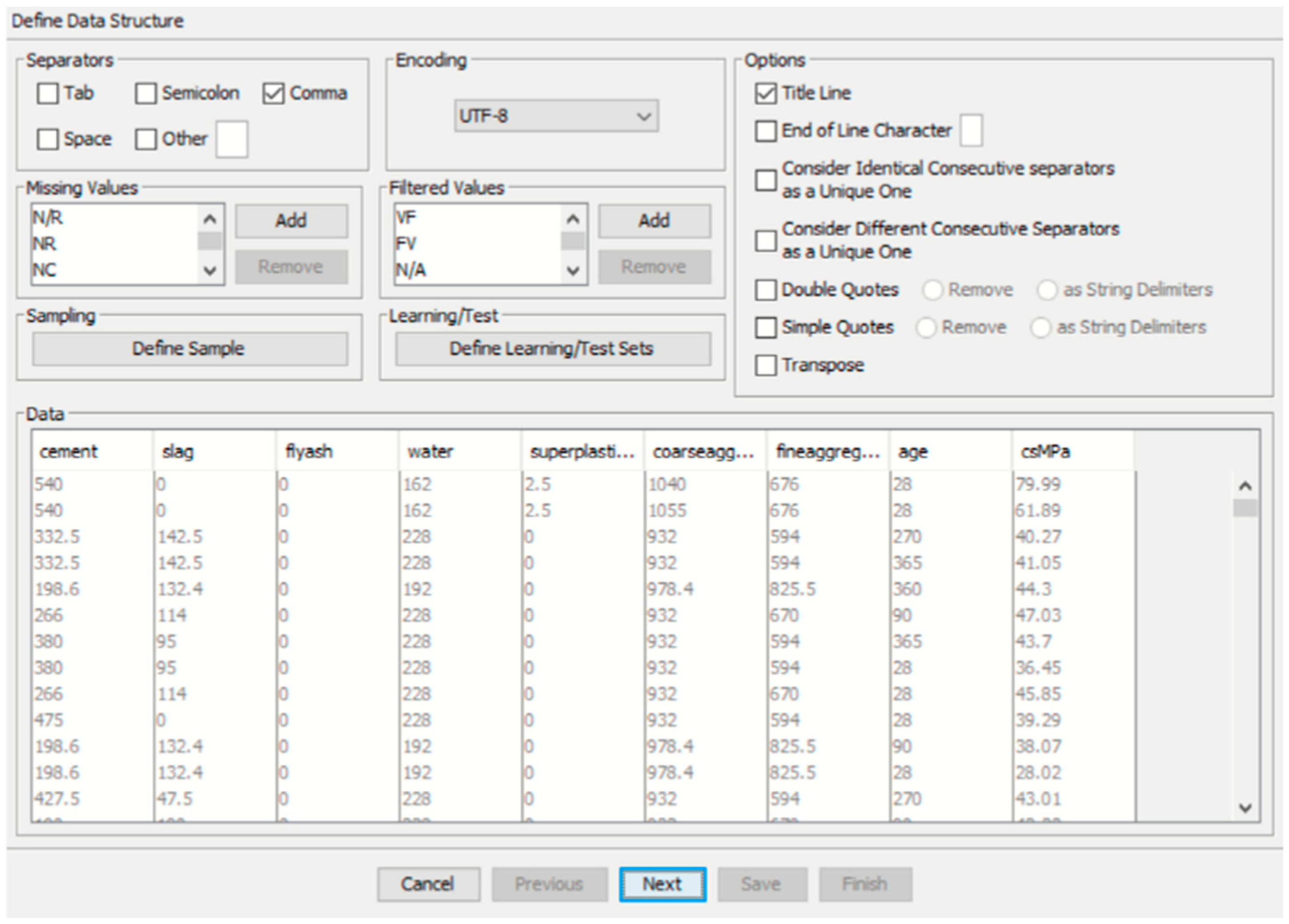
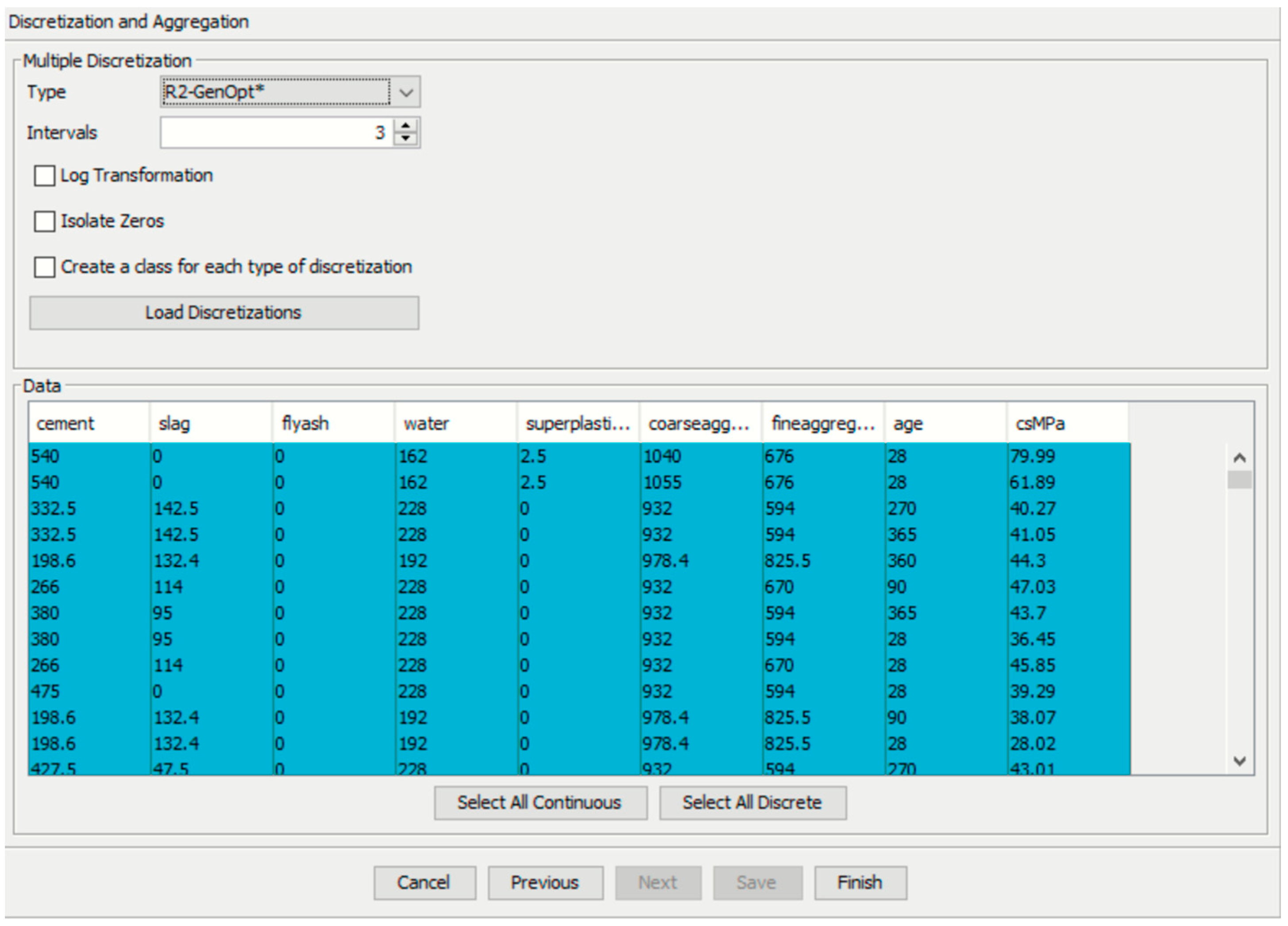
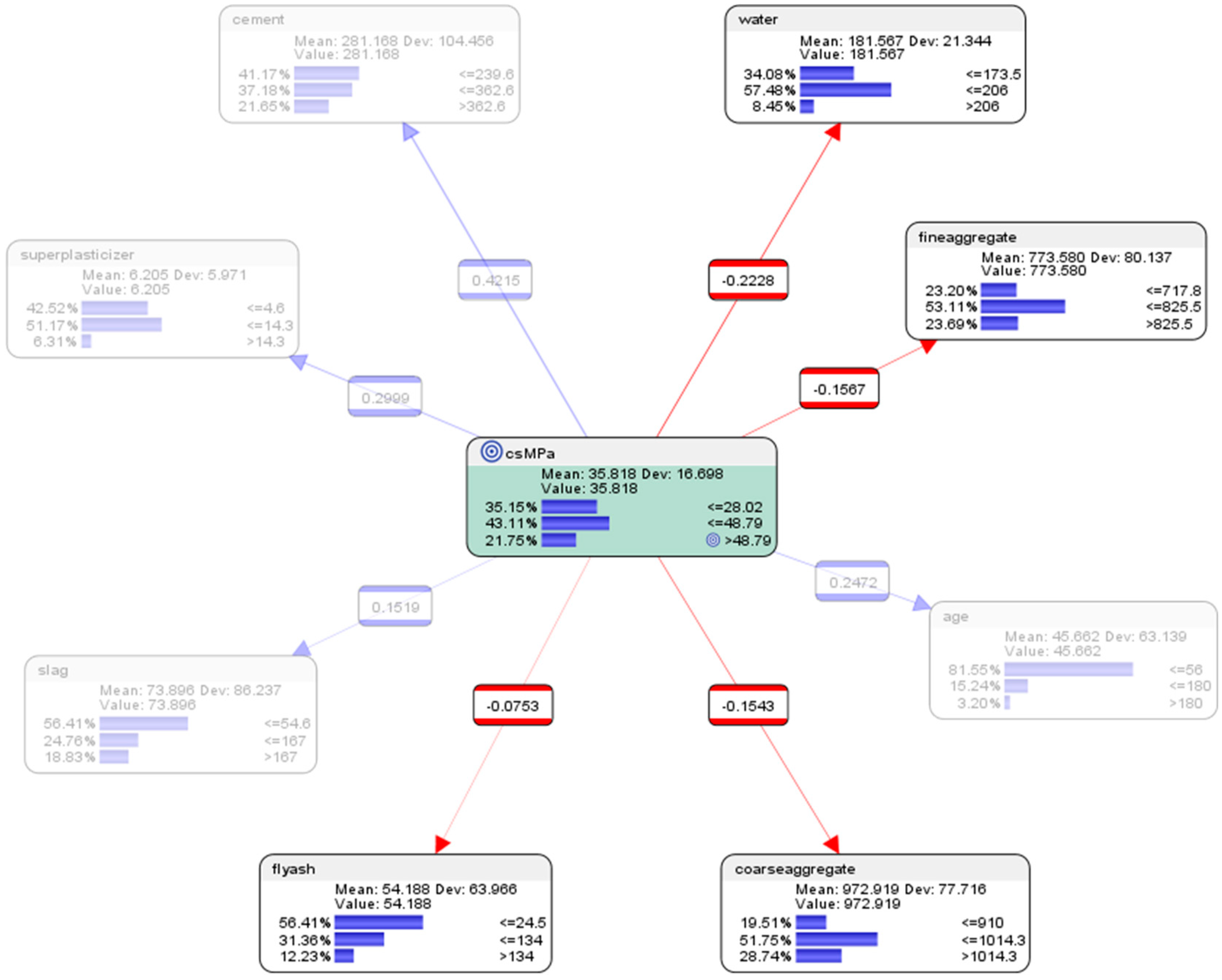
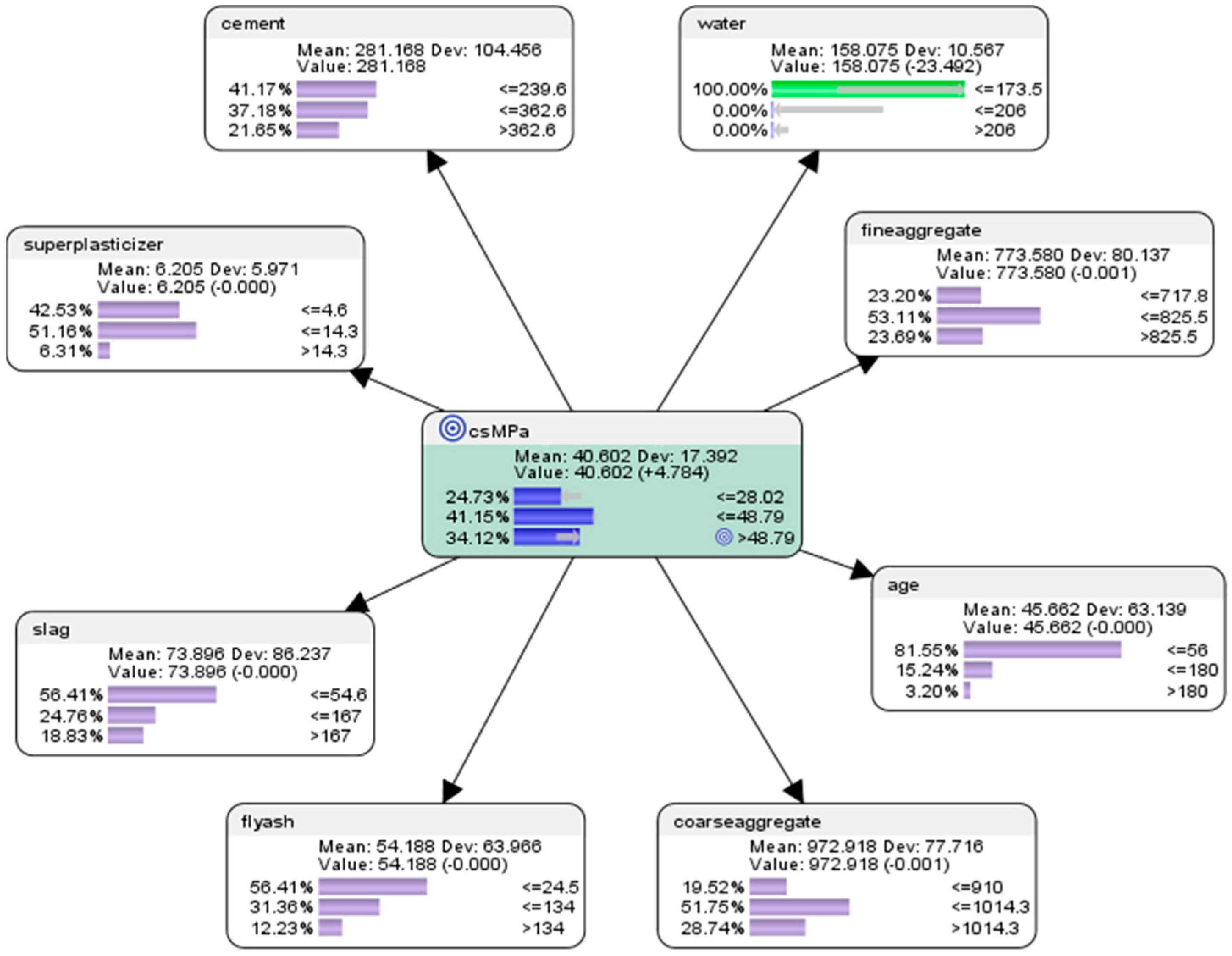
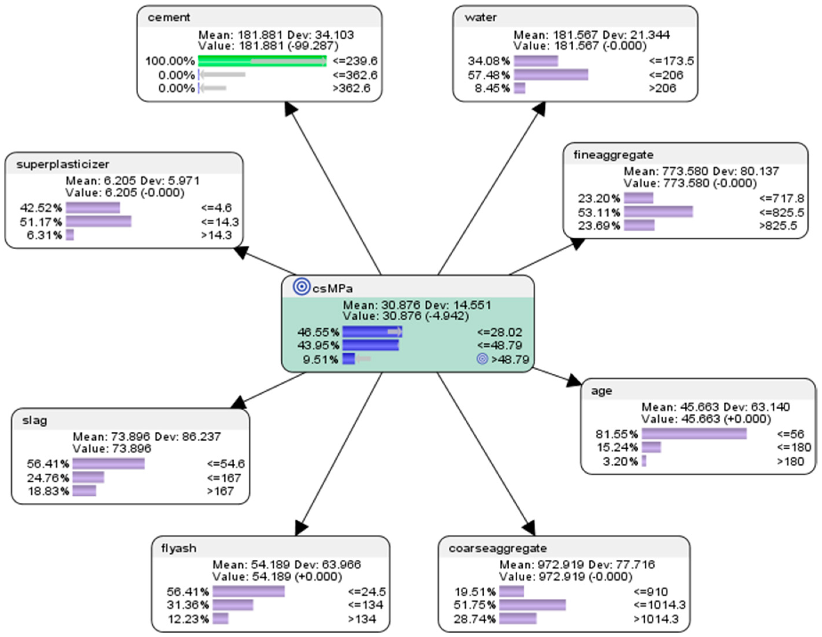
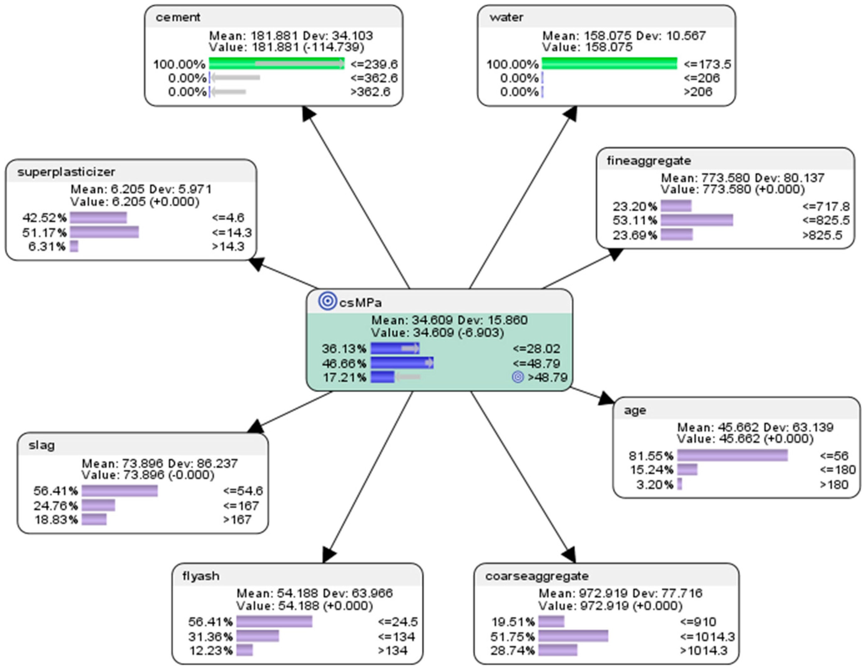
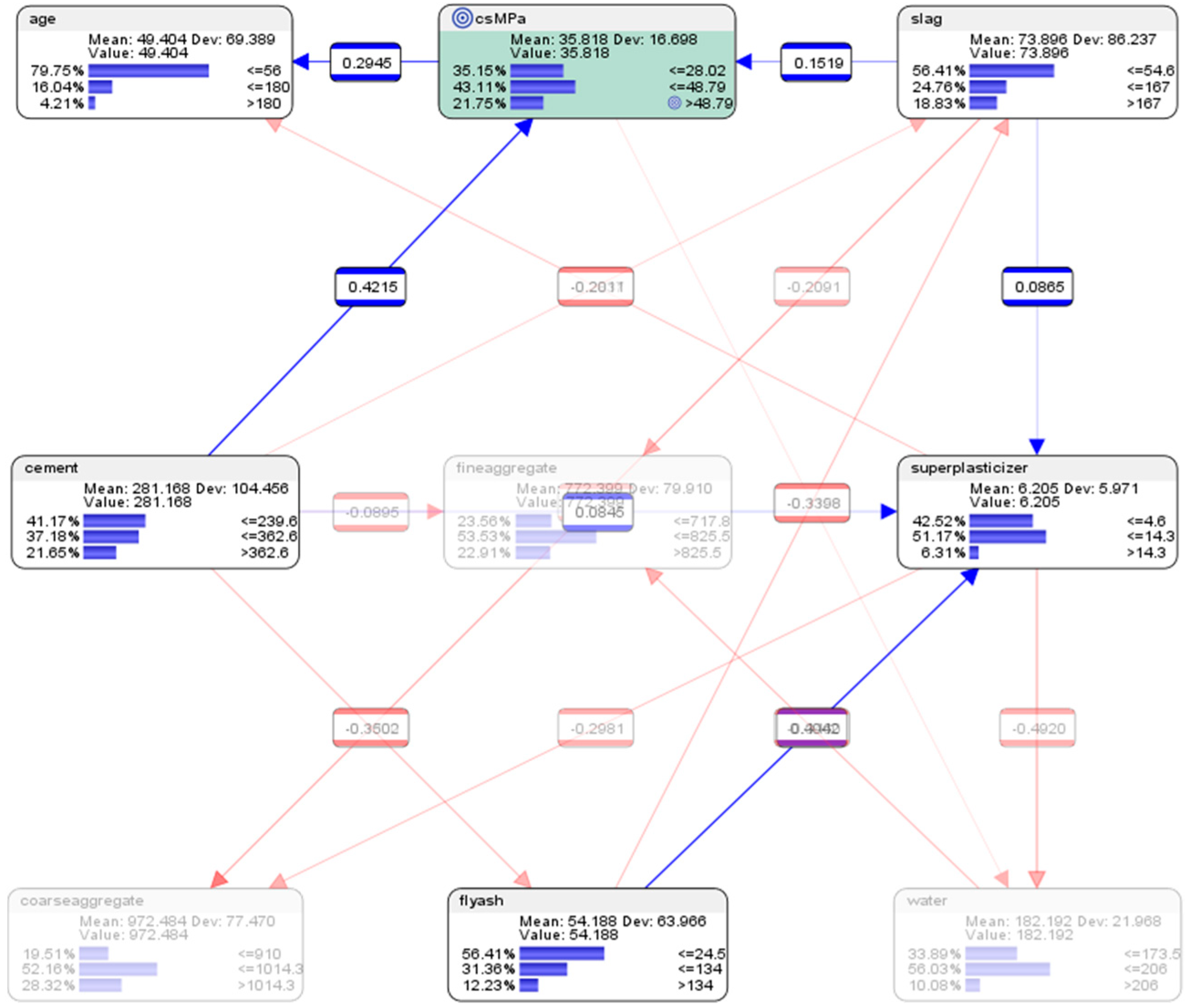
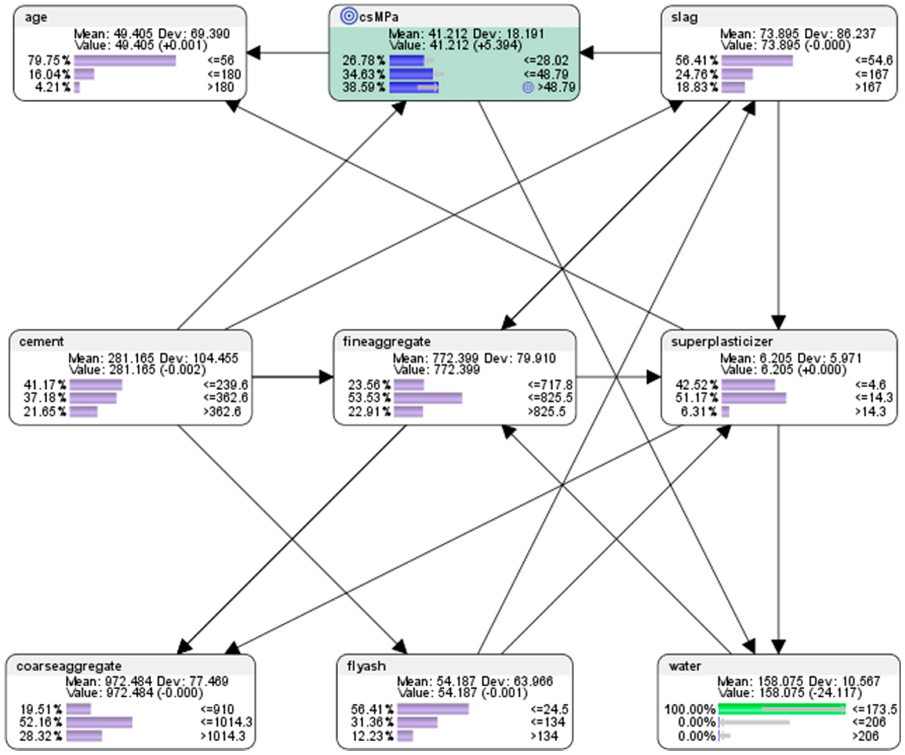
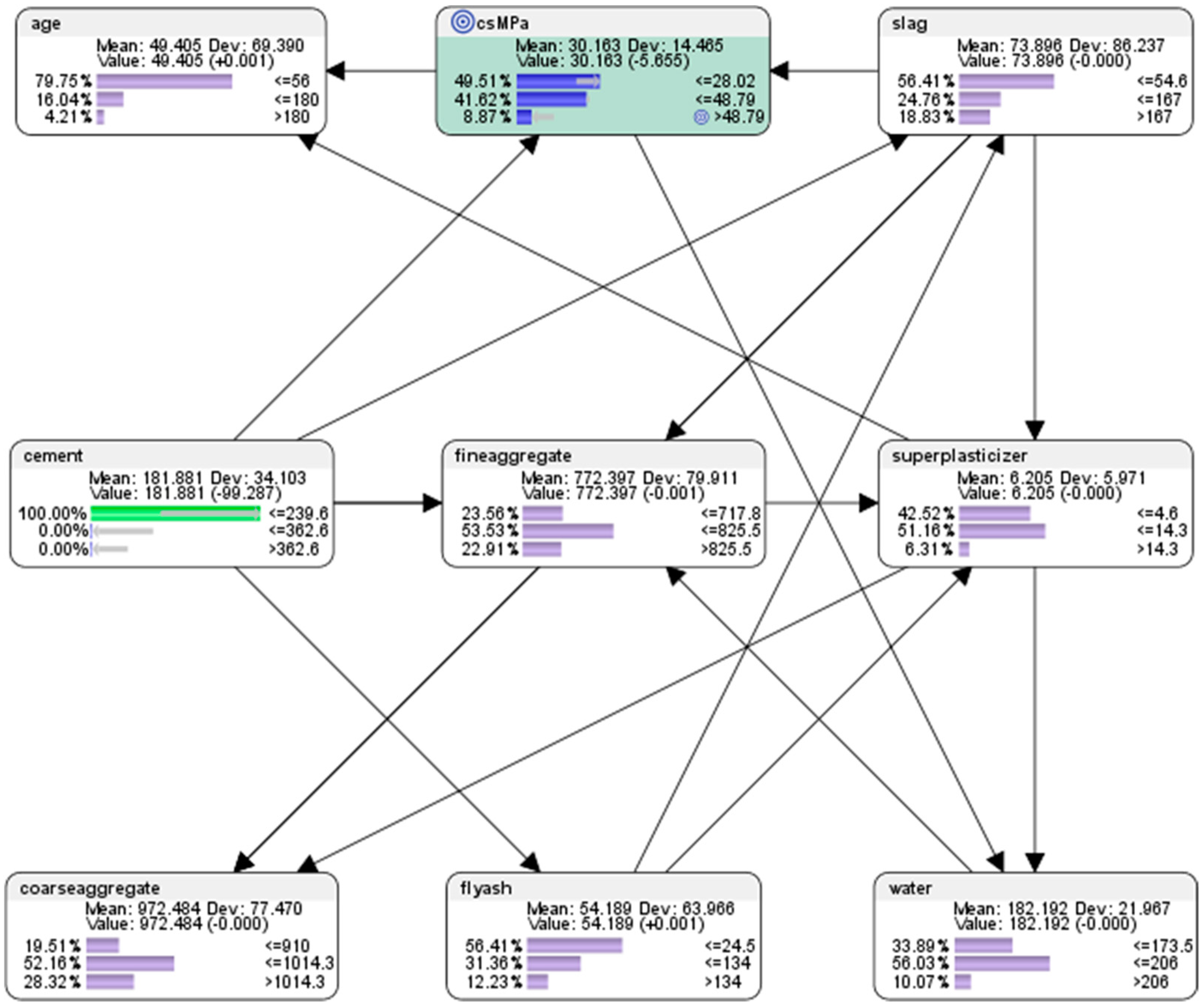
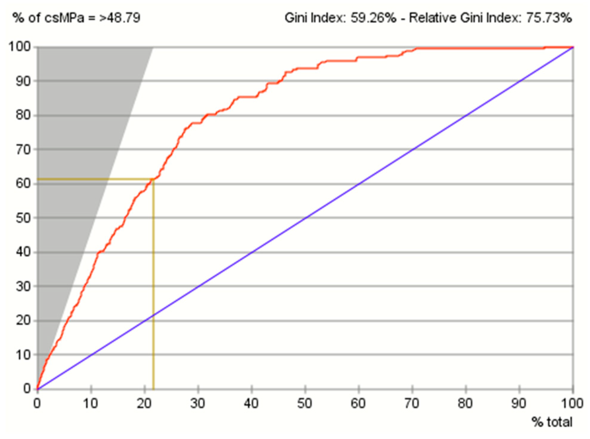
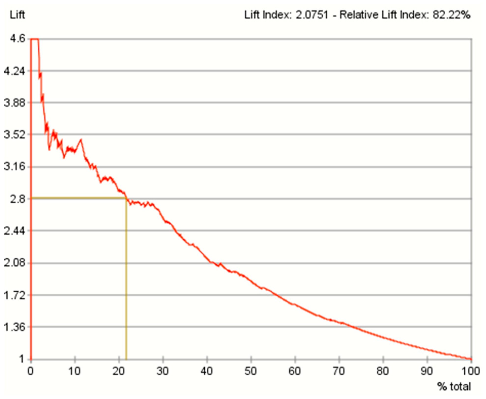
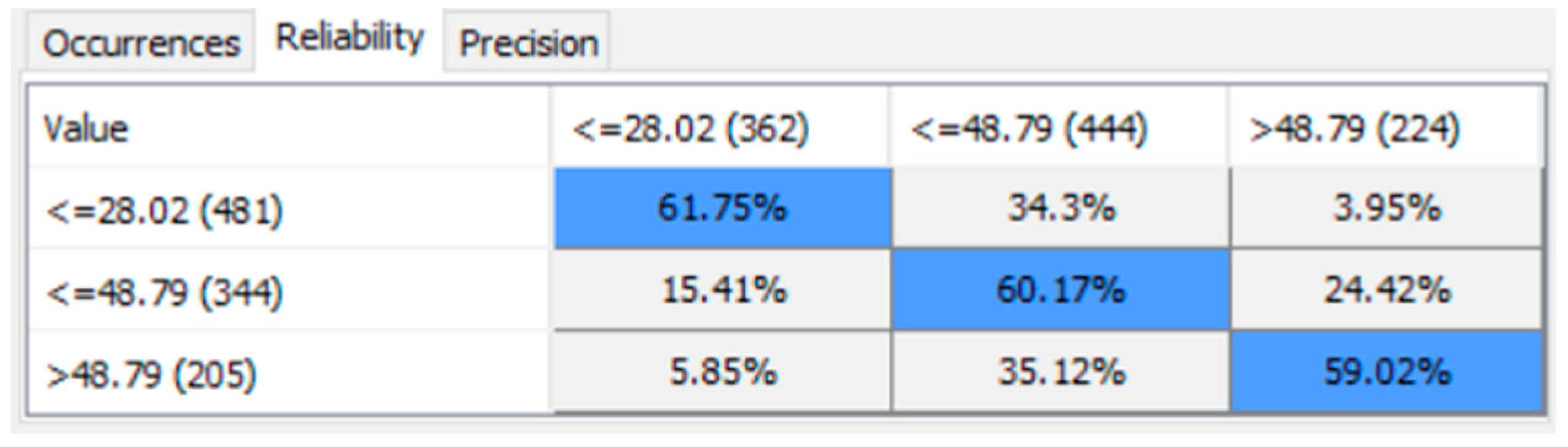
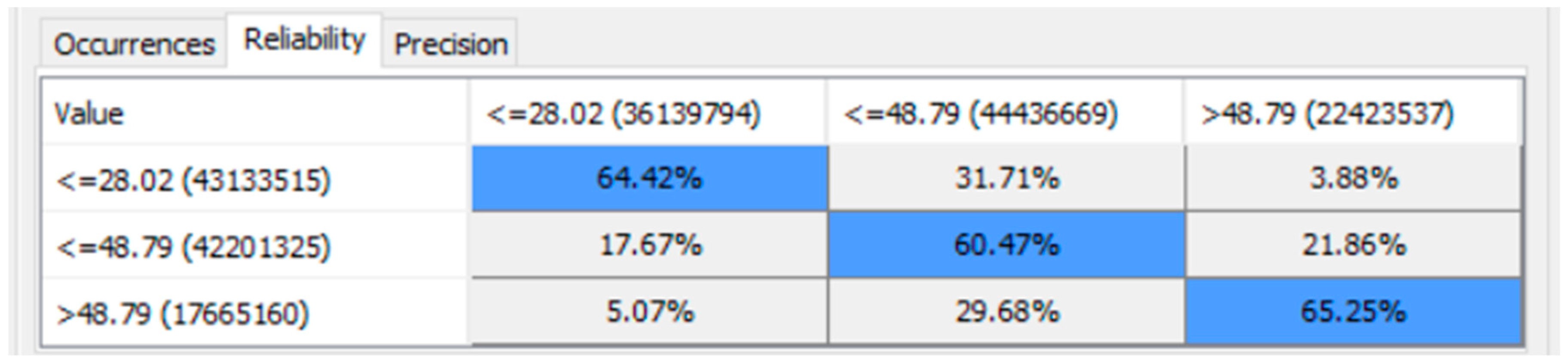
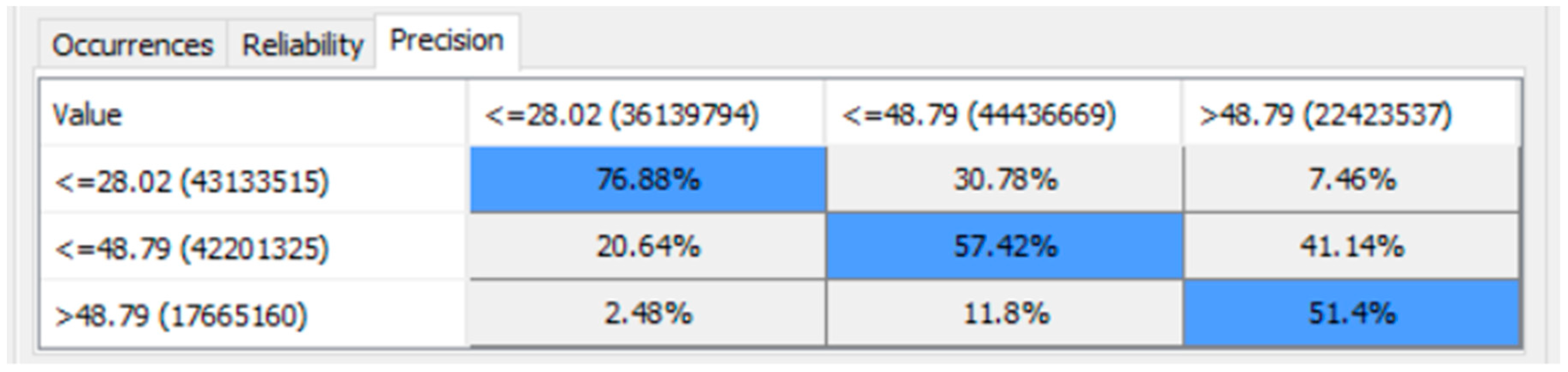
Table 1.
Code book of the data.
| Name | Description |
|---|---|
| Cement | input variable: Kg in a m3 mixture |
| Blast Furnace Slag | input variable: Kg in a m3 mixture |
| Fly Ash | input variable: Kg in a m3 mixture |
| Water | input variable: Kg in a m3 mixture |
| Superplasticizer | input variable: Kg in a m3 mixture |
| Coarse Aggregate | input variable: Kg in a m3 mixture |
| Fine Aggregate | input variable: Kg in a m3 mixture |
| Age | input variable: Day (1~365) |
| Concrete compressive strength | Output variable: MPa |
Table 2.
Relationship between parent and child nodes of the supervised machine-learned BN.
| Parent | Child | KL Divergence | Mutual Information | G-Test | df | p-Value | Pearson’s Correlation |
|---|---|---|---|---|---|---|---|
| csMPa | cement | 0.1359 | 0.1359 | 194.0049 | 4 | 0.0000% | 0.4215 |
| csMPa | water | 0.1125 | 0.1125 | 160.6493 | 4 | 0.0000% | −0.2228 |
| csMPa | age | 0.0891 | 0.0891 | 127.2237 | 4 | 0.0000% | 0.2472 |
| csMPa | superplasticizer | 0.0689 | 0.0689 | 98.3567 | 4 | 0.0000% | 0.2999 |
| csMPa | fineaggregate | 0.0260 | 0.0260 | 37.1368 | 4 | 0.0000% | −0.1567 |
| csMPa | coarseaggregate | 0.0208 | 0.0208 | 29.6499 | 4 | 0.0006% | −0.1543 |
| csMPa | slag | 0.0206 | 0.0206 | 29.3990 | 4 | 0.0006% | 0.1519 |
| csMPa | flyash | 0.0186 | 0.0186 | 26.5392 | 4 | 0.0025% | −0.0753 |
Table 3.
Relationship analysis between parent and child nodes in the semi-supervised machine-learned BN.
Table 3.
Relationship analysis between parent and child nodes in the semi-supervised machine-learned BN.
| Parent | Child | KL Divergence | Mutual Information | G-Test | df | p-Value | Pearson’s Correlation |
|---|---|---|---|---|---|---|---|
| flyash | superplasticizer | 0.4372 | 0.3004 | 428.9930 | 4 | 0.0000% | 0.4042 |
| fineaggregate | coarseaggregate | 0.3303 | 0.1275 | 193.7040 | 4 | 0.0000% | −0.1800 |
| cement | fineaggregate | 0.3037 | 0.0255 | 53.7375 | 4 | 0.0000% | −0.0895 |
| water | fineaggregate | 0.2930 | 0.1155 | 198.8320 | 4 | 0.0000% | −0.3460 |
| slag | fineaggregate | 0.2792 | 0.0450 | 72.3311 | 4 | 0.0000% | −0.2091 |
| superplasticizer | water | 0.2514 | 0.2254 | 356.7480 | 4 | 0.0000% | −0.4920 |
| slag | coarseaggregate | 0.2434 | 0.0825 | 129.5773 | 4 | 0.0000% | −0.2844 |
| flyash | slag | 0.2238 | 0.1289 | 183.9886 | 4 | 0.0000% | −0.3398 |
| cement | csMPa | 0.2226 | 0.1359 | 194.0049 | 4 | 0.0000% | 0.4215 |
| slag | superplasticizer | 0.2187 | 0.0338 | 48.3312 | 4 | 0.0000% | 0.0865 |
| superplasticizer | coarseaggregate | 0.2086 | 0.0891 | 106.7541 | 4 | 0.0000% | −0.2981 |
| cement | superplasticizer | 0.1989 | 0.0739 | 105.5544 | 4 | 0.0000% | 0.0845 |
| csMPa | age | 0.1464 | 0.1160 | 127.2237 | 4 | 0.0000% | 0.2945 |
| cement | slag | 0.1304 | 0.0355 | 50.6310 | 4 | 0.0000% | −0.2011 |
| superplasticizer | age | 0.1240 | 0.0936 | 81.2284 | 4 | 0.0000% | −0.2837 |
| cement | flyash | 0.1158 | 0.1158 | 165.4023 | 4 | 0.0000% | −0.3502 |
| slag | csMPa | 0.1073 | 0.0206 | 29.3990 | 4 | 0.0006% | 0.1519 |
| csMPa | water | 0.1041 | 0.0781 | 160.6493 | 4 | 0.0000% | −0.1156 |
© 2019 by the authors. Licensee MDPI, Basel, Switzerland. This article is an open access article distributed under the terms and conditions of the Creative Commons Attribution (CC BY) license (http://creativecommons.org/licenses/by/4.0/).
Share and Cite
MDPI and ACS Style
How, M.-L.; Hung, W.L.D. Educing AI-Thinking in Science, Technology, Engineering, Arts, and Mathematics (STEAM) Education. Educ. Sci. 2019, 9, 184. https://doi.org/10.3390/educsci9030184
AMA Style
How M-L, Hung WLD. Educing AI-Thinking in Science, Technology, Engineering, Arts, and Mathematics (STEAM) Education. Education Sciences. 2019; 9(3):184. https://doi.org/10.3390/educsci9030184
Chicago/Turabian StyleHow, Meng-Leong, and Wei Loong David Hung. 2019. "Educing AI-Thinking in Science, Technology, Engineering, Arts, and Mathematics (STEAM) Education" Education Sciences 9, no. 3: 184. https://doi.org/10.3390/educsci9030184
Note that from the first issue of 2016, this journal uses article numbers instead of page numbers. See further details here.