Proteomic Workflows for Biomarker Identification Using Mass Spectrometry — Technical and Statistical Considerations during Initial Discovery

Abstract
:1. Introduction
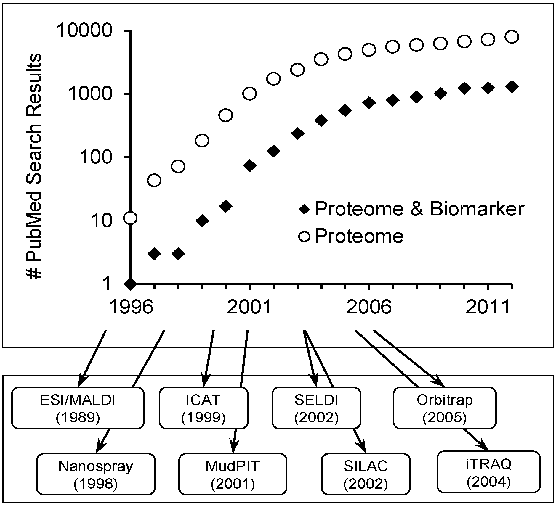
Scope of Review
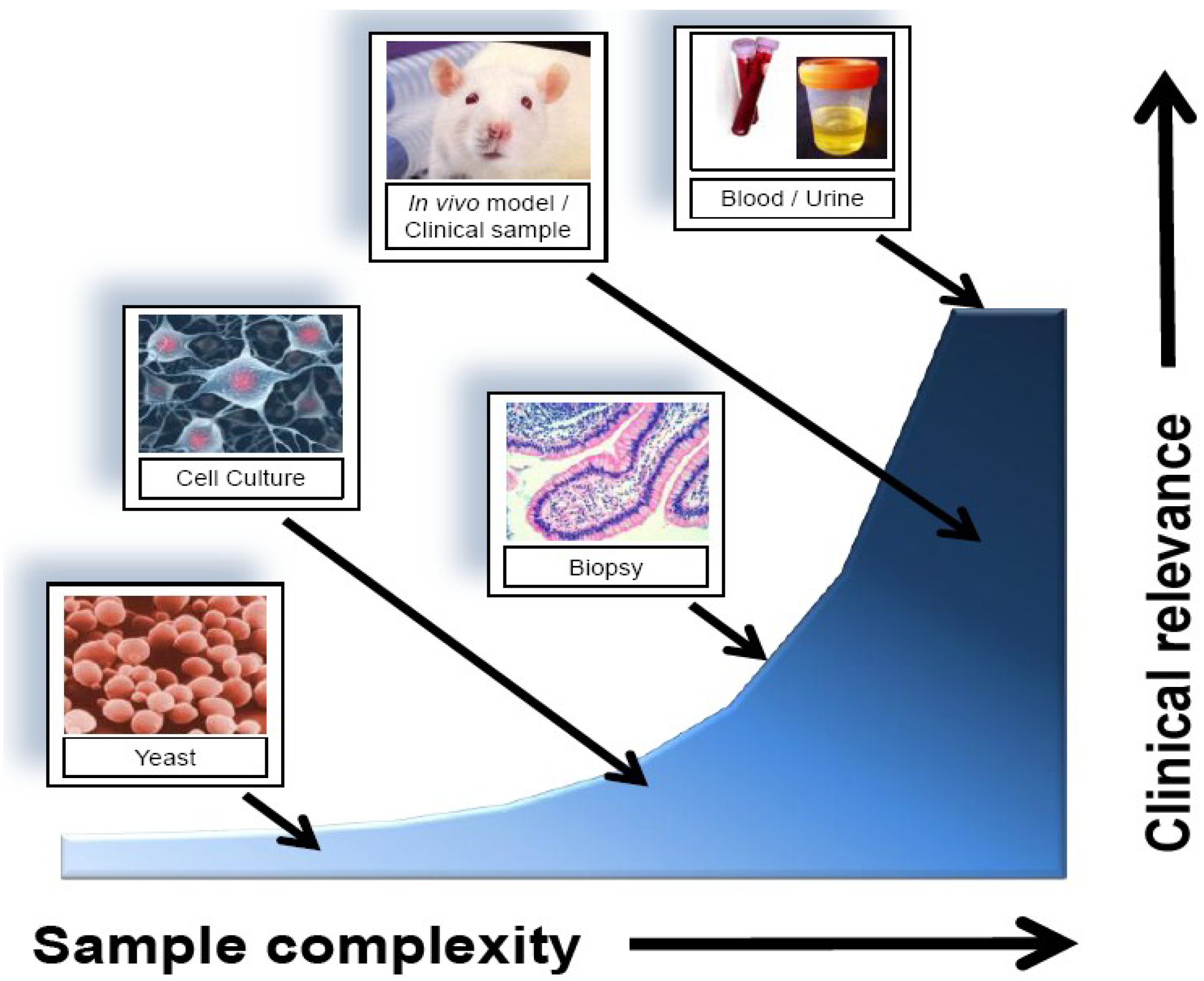
2. Sample Description
2.1. Characteristics of an Ideal Biomarker

| Characteristic | Description |
|---|---|
| (1) Non-invasive collection | Expression within a sample obtainable without discomfort to the patient |
| (2) Readily available | Presentation in an easily obtainable sample that is commonly obtained clinically such as blood or urine |
| (3) High sensitivity | Allows early detection of disease with little or no overlap between healthy and diseased patients |
| (4) High specificity | Present in the disease in question, with little or no overlap between comorbid conditions |
| (5) Rapid response | Changes rapidly in response to treatment |
| (6) Risk stratification | Provides prognostic information to the clinician, allowing classification of the disease along with diagnosis |
| (7) Insight to disease | Provides insight into the underlying mechanism of the disease |
2.2. Sources for Biomarker Identification
| Source | Advantages | Disadvantages |
|---|---|---|
| In vitro cell culture | Easy to obtain; no ethics; abundant sample quantity; good for characterizing cell-specific responses | Lack of heterogeneity; may not represent clinically relevant results |
| Tissue biopsy/core sample | Accessibility to samples stored long term; direct comparison to standard diagnosis; tissue-level representative profiling | Potential for sample degradation; require large validation datasets; invasive sample collection |
| Urine/blood | Easy to obtain; express representative protein and gene expression of a large number of cell types | Low marker concentration; high sample complexity; technically difficult to detect |
| Proximal fluid (e.g., Nipple aspirate, bile, prostate, etc…) | Representative of the tissue microenvironment over blood/urine; may provide more sensitive results | More difficult to obtain than blood/urine; potentially extremely invasive (e.g., CSF) |
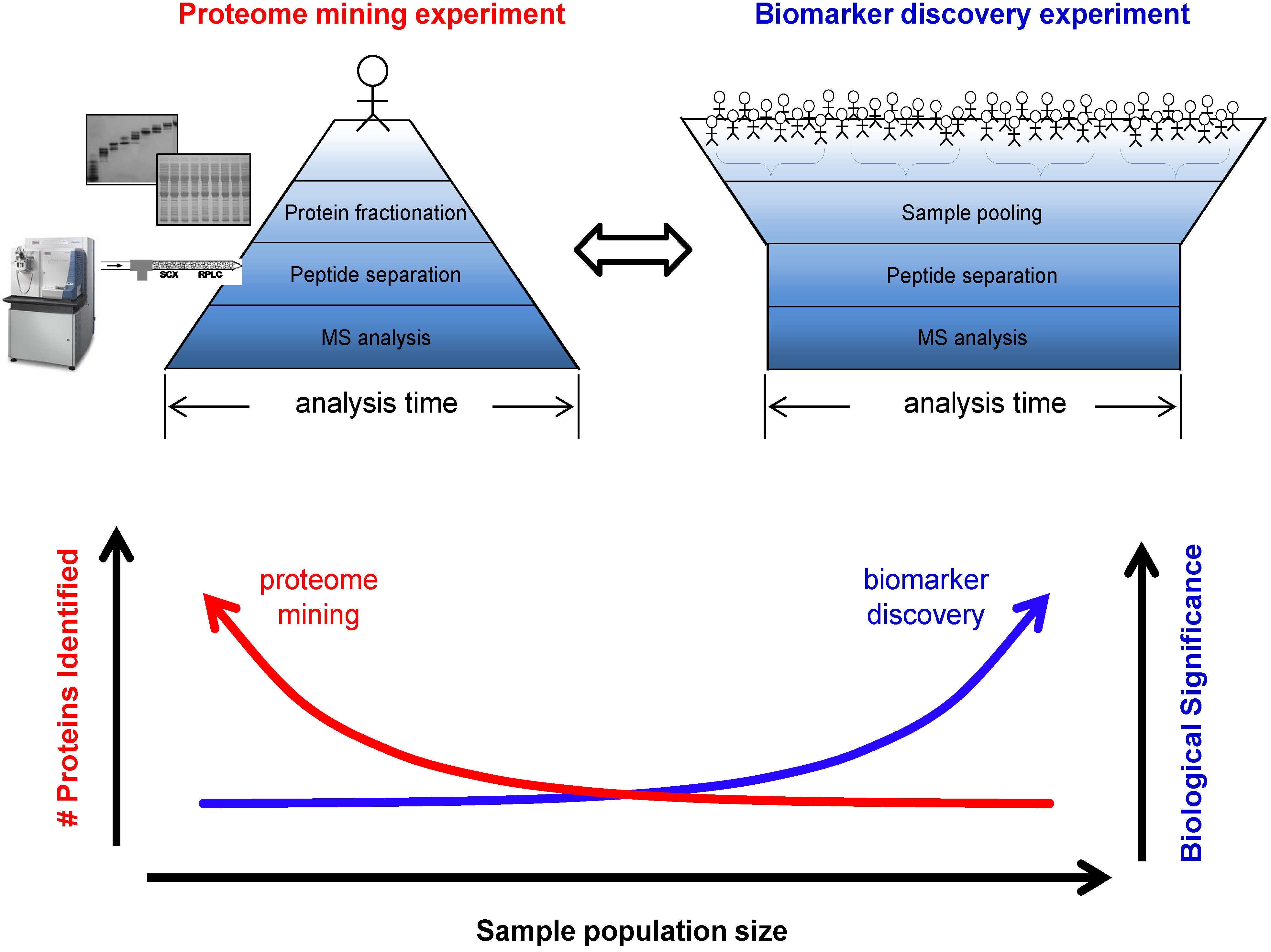
3. Sample Analysis
3.1. Biomarker Discovery Experimental Design
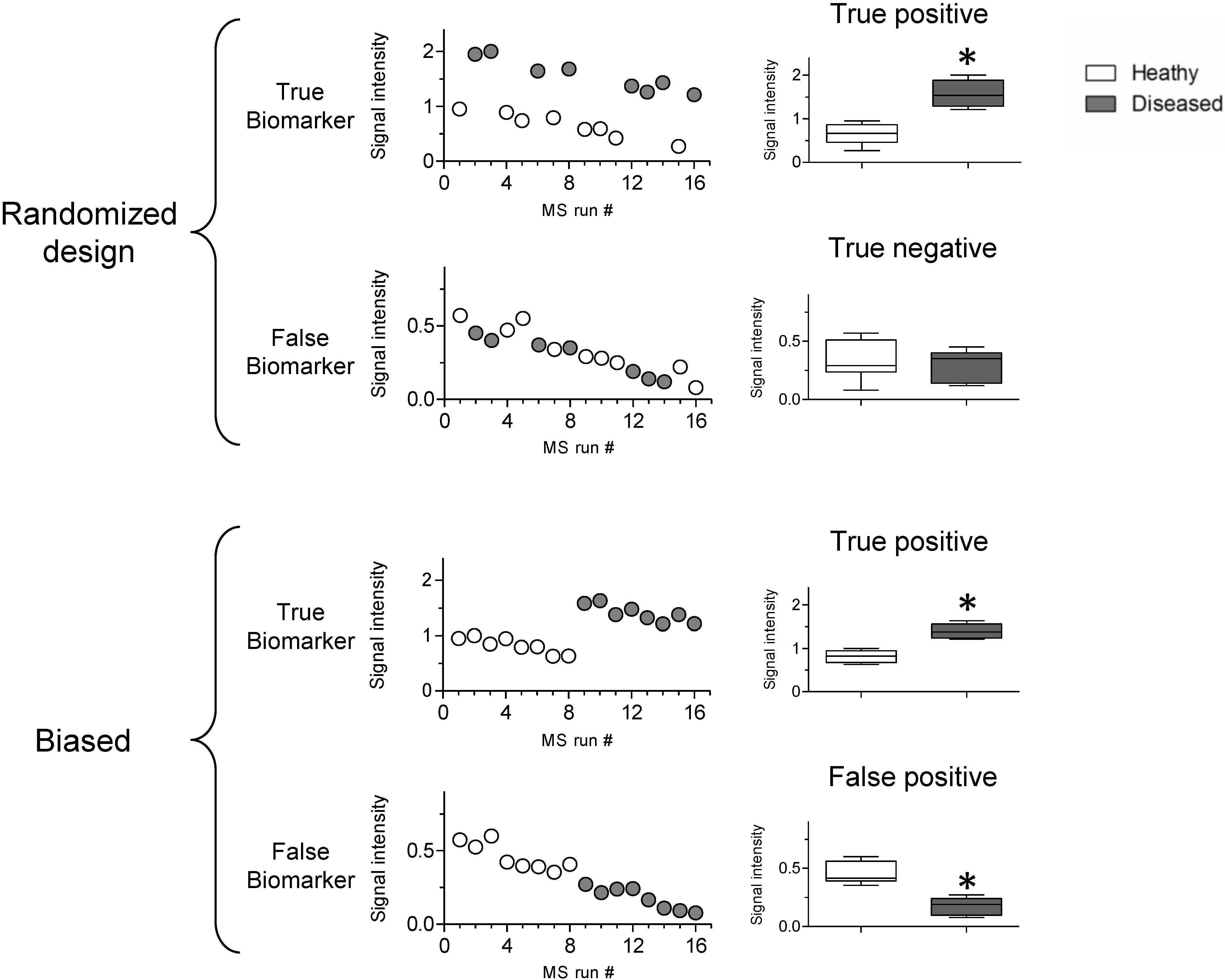

3.2. Sources of Bias
3.3. Statistical Analysis of High Dimensional Datasets
4. Conclusions
Acknowledgments
Conflicts of Interest
References
- Rosenberg, S.; Elashoff, M.R.; Beineke, P.; Daniels, S.E.; Wingrove, J.A.; Tingley, W.G.; Sager, P.T.; Sehnert, A.J.; Yau, M.; Kraus, W.E.; et al. Multicenter validation of the diagnostic accuracy of a blood-based gene expression test for assessing obstructive coronary artery disease in nondiabetic patients. Ann. Int. Med. 2010, 153, 425–434. [Google Scholar] [CrossRef]
- Dumur, C.I.; Lyons-Weiler, M.; Sciulli, C.; Garrett, C.T.; Schrijver, I.; Holley, T.K.; Rodriguez-Paris, J.; Pollack, J.R.; Zehnder, J.L.; Price, M.; et al. Interlaboratory performance of a microarray-based gene expression test to determine tissue of origin in poorly differentiated and undifferentiated cancers. J. Mol. Diagn. 2008, 10, 67–77. [Google Scholar] [CrossRef]
- Cronin, M.; Pho, M.; Dutta, D.; Stephans, J.C.; Shak, S.; Kiefer, M.C.; Esteban, J.M.; Baker, J.B. Measurement of gene expression in archival paraffin-embedded tissues: Development and performance of a 92-gene reverse transcriptase-polymerase chain reaction assay. Am. J. Pathol. 2004, 164, 35–42. [Google Scholar] [CrossRef]
- Bedard, P.L.; Mook, S.; Piccart-Gebhard, M.J.; Rutgers, E.T.; Van’t Veer, L.J.; Cardoso, F. MammaPrint 70-gene profile quantifies the likelihood of recurrence for early breast cancer. Expert Opin. Med. Diagn. 2009, 3, 193–205. [Google Scholar] [CrossRef]
- Deng, M.C.; Eisen, H.J.; Mehra, M.R.; Billingham, M.; Marboe, C.C.; Berry, G.; Kobashigawa, J.; Johnson, F.L.; Starling, R.C.; Murali, S.; et al. Noninvasive discrimination of rejection in cardiac allograft recipients using gene expression profiling. Am. J. Transplant. 2006, 6, 150–160. [Google Scholar] [CrossRef]
- Ueland, F.R.; Desimone, C.P.; Seamon, L.G.; Miller, R.A.; Goodrich, S.; Podzielinski, I.; Sokoll, L.; Smith, A.; van Nagell, J.R.; Zhang, Z. Effectiveness of a multivariate index assay in the preoperative assessment of ovarian tumors. Obstet. Gynecol. 2011, 117, 1289–1297. [Google Scholar] [CrossRef]
- DeSouza, L.V.; Siu, K.W.M. Mass spectrometry-based quantification. Clin. Biochem. 2013, 46, 421–431. [Google Scholar] [CrossRef]
- De Godoy, L.M.F.; Olsen, J.V.; Cox, J.; Nielsen, M.L.; Hubner, N.C.; Fröhlich, F.; Walther, T.C.; Mann, M. Comprehensive mass-spectrometry-based proteome quantification of haploid versus diploid yeast. Nature 2008, 455, 1251–1254. [Google Scholar] [CrossRef]
- Fenn, J.B.; Mann, M.; Meng, C.K.; Wong, S.F.; Whitehouse, C.M. Electrospray ionization of large for mass spectrometry biomolecules. Science 1989, 246, 64–71. [Google Scholar]
- Gatlin, C.L.; Kleemann, G.R.; Hays, L.G.; Link, A.J.; Yates, J.R., III. Protein identification at the low femtomole level from silver-stained gels using a new fritless electrospray interface for liquid chromatography-microspray and nanospray mass spectrometry. Anal. Biochem. 1998, 263, 93–101. [Google Scholar] [CrossRef]
- Gygi, S.P.; Rist, B.; Gerber, S.A.; Turecek, F.; Gelb, M.H.; Aebersold, R. Quantitative analysis of complex protein mixtures using isotope-coded affinity tags. Nat. Biotechnol. 1999, 10, 994–999. [Google Scholar]
- Washburn, M.P.; Wolters, D.; Yates, J.R., III. Large-scale analysis of the yeast proteome by multidimensional protein identification technology. Nat. Biotechnol. 2001, 3, 242–247. [Google Scholar] [CrossRef]
- Issaq, H.J.; Veenstra, T.D.; Conrads, T.P.; Felschow, D. The SELDI-TOF MS approach to proteomics: Protein profiling and biomarker identification. Biochem. Biophys. Res. Commun. 2002, 292, 587–592. [Google Scholar] [CrossRef]
- Ong, S.E.; Blagoev, B.; Kratchmarova, I.; Kristensen, D.B.; Steen, H.; Pandey, A.; Mann, M. Stable isotope labeling by amino acids in cell culture, SILAC, as a simple and accurate approach to expression proteomics. Mol. Cell. Proteomics 2002, 1, 376–386. [Google Scholar] [CrossRef]
- Wiese, S.; Reidegeld, K.A.; Meyer, H.E.; Warscheid, B. Protein labeling by iTRAQ: A new tool for quantitative mass spectrometry in proteome research. Proteomics 2007, 7, 340–350. [Google Scholar] [CrossRef]
- Olsen, J.V.; de Godoy, L.M.F.; Li, G.; Macek, B.; Mortensen, P.; Pesch, R.; Makarov, A.; Lange, O.; Horning, S.; Mann, M. Parts per million mass accuracy on an Orbitrap mass spectrometer via lock mass injection into a C-trap. Mol. Cell. Proteomics 2005, 4, 2010–2021. [Google Scholar] [CrossRef]
- Reddy, M.M.; Wilson, R.; Wilson, J.; Connell, S.; Gocke, A.; Hynan, L.; German, D.; Kodadek, T. Identification of candidate IgG biomarkers for Alzheimer’s disease via combinatorial library screening. Cell 2011, 144, 132–142. [Google Scholar] [CrossRef]
- Pepe, M.S.; Feng, Z. Improving biomarker identification with better designs and reporting. Clin. Chem. 2011, 57, 1093–1095. [Google Scholar] [CrossRef]
- Hu, J.; Coombes, K.R.; Morris, J.S.; Baggerly, K.A. The importance of experimental design in proteomic mass spectrometry experiments: Some cautionary tales. Brief. Funct. Genomic. Proteomics 2005, 3, 322–331. [Google Scholar] [CrossRef]
- Banks, R.E.; Stanley, A.J.; Cairns, D.A.; Barrett, J.H.; Clarke, P.; Thompson, D.; Selby, P.J. Influences of blood sample processing on low-molecular-weight proteome identified by surface-enhanced laser desorption/ionization mass spectrometry. Clin. Chem. 2005, 51, 1637–1649. [Google Scholar] [CrossRef]
- Leitch, M.C.; Mitra, I.; Sadygov, R.G. Generalized linear and mixed models for label-free shotgun proteomics. Stat. Interface 2012, 5, 89–98. [Google Scholar]
- Johnstone, I.M.; Titterington, D.M. Statistical challenges of high-dimensional data. Philos. Trans. R. Soc. A 2009, 367, 4237–4253. [Google Scholar] [CrossRef]
- Clarke, R.; Ressom, H.W.; Wang, A.; Xuan, J.; Liu, M.C.; Gehan, E.A.; Wang, Y. The properties of high-dimensional data spaces: Implications for exploring gene and protein expression data. Nat. Rev. Cancer 2008, 8, 37–49. [Google Scholar] [CrossRef]
- Petricoin, E.F.I.; Ardekani, A.M.; Hitt, B.A.; Levine, P.J.; Fusaro, V.A.; Steinberg, S.M.; Mills, G.B.; Simone, C.; Fishman, D.A.; Kohn, E.C.; et al. Use of proteomic patterns in serum to identify ovarian cancer. Lancet 2002, 359, 572–577. [Google Scholar] [CrossRef]
- Adam, B.L.; Qu, Y.; Davis, J.W.; Ward, M.D.; Clements, M.A.; Cazares, L.H.; Semmes, O.J.; Schellhammer, P.F.; Yasui, Y.; Feng, Z.; et al. Serum protein fingerprinting coupled with a pattern-matching algorithm distinguishes prostate cancer from benign prostate hyperplasia and healthy men. Cancer Res. 2002, 62, 3609–3614. [Google Scholar]
- McLerran, D.; Grizzle, W.E.; Feng, Z.; Bigbee, W.L.; Banez, L.L.; Cazares, L.H.; Chan, D.W.; Diaz, J.; Izbicka, E.; Kagan, J.; et al. Analytical validation of serum proteomic profiling for diagnosis of prostate cancer: Sources of sample bias. Clin. Chem. 2008, 54, 44–52. [Google Scholar]
- McLerran, D.; Grizzle, W.E.; Feng, Z.; Thompson, I.M.; Bigbee, W.L.; Cazares, L.H.; Chan, D.W.; Dahlgren, J.; Diaz, J.; Kagan, J.; et al. SELDI-TOF MS whole serum proteomic profiling with IMAC surface does not reliably detect prostate cancer. Clin. Chem. 2008, 54, 53–60. [Google Scholar]
- Rifai, N.; Gillette, M.A.; Carr, S.A. Protein biomarker discovery and validation: The long and uncertain path to clinical utility. Nat. Biotechnol. 2006, 24, 971–983. [Google Scholar] [CrossRef]
- Ransohoff, D.F. Rules of evidence for cancer molecular-marker discovery and validation. Nat. Rev. Cancer 2004, 4, 309–314. [Google Scholar] [CrossRef]
- Mischak, H.; Ioannidis, J.P.; Argiles, A.; Attwood, T.K.; Bongcam-Rudloff, E.; Broenstrup, M.; Charonis, A.; Chrousos, G.P.; Delles, C.; Dominiczak, A.; et al. Implementation of proteomic biomarkers: Making it work. Eur. J. Clin. Invest. 2012, 42, 1027–1036. [Google Scholar] [CrossRef]
- Atkinson, A.J.; Colburn, W.A.; DeGruttola, V.G.; DeMets, D.L.; Downing, G.J.; Hoth, D.F.; Oates, J.A.; Peck, C.C.; Schooley, R.T.; Spilker, B.A.; et al. Biomarkers and surrogate endpoints: Preferred definitions and conceptual framework. J. Clin. Pharm. Ther. 2001, 69, 89–95. [Google Scholar] [CrossRef]
- Paik, S.; Shak, S.; Tang, G.; Kim, C.; Baker, J.; Cronin, M.; Baehner, F.L.; Walker, M.G.; Watson, D.; Park, T.; et al. A multigene assay to predict recurrence of tamoxifen-treated, node-negative breast cancer. N. Engl. J. Med. 2004, 351, 2817–2826. [Google Scholar] [CrossRef]
- Jiang, F.; Katz, R.L. Use of interphase fluorescence in situ hybridization as a powerful diagnostic tool in cytology. Diagn. Mol. Pathol. 2002, 11, 47–57. [Google Scholar] [CrossRef]
- Schena, M.; Shalon, D.; Davis, R.W.; Brown, P.O. Quantitative monitoring of gene expression patterns with a complementary DNA microarray. Science 1995, 270, 467–470. [Google Scholar]
- Stevens, T.; Berk, M.P.; Lopez, R.; Chung, Y.M.; Zhang, R.; Parsi, M.A.; Bronner, M.P.; Feldstein, A.E. Lipidomic profiling of serum and pancreatic fluid in chronic pancreatitis. Pancreas 2012, 41, 518–522. [Google Scholar] [CrossRef]
- Anderson, N.L. The human plasma proteome: History, character, and diagnostic prospects. Mol. Cell. Proteomics 2002, 1, 845–867. [Google Scholar] [CrossRef]
- Nilsson, T.; Mann, M.; Aebersold, R.; Yates, J.R., III; Bairoch, A.; Bergeron, J.J. Mass spectrometry in high-throughput proteomics: Ready for the big time. Nat. Methods 2010, 7, 681–685. [Google Scholar] [CrossRef]
- Kim, Y.S.; Maruvada, P.; Milner, J.A. Metabolomics in biomarker discovery: Future uses for cancer prevention. Future Oncol. 2008, 4, 93–102. [Google Scholar] [CrossRef]
- MacLellan, D.L.; Mataija, D.; Doucette, A.; Huang, W.; Langlois, C.; Trottier, G.; Burton, I.W.; Walter, J.A.; Karakach, T.K. Alterations in urinary metabolites due to unilateral ureteral obstruction in a rodent model. Mol. Biosyst. 2011, 7, 2181–2188. [Google Scholar] [CrossRef]
- Paulo, J.A.; Urrutia, R.; Banks, P.A.; Conwell, D.L.; Steen, H. Proteomic analysis of an immortalized mouse pancreatic stellate cell line identifies differentially-expressed proteins in activated vs. nonproliferating cell states. J. Proteome Res. 2011, 10, 4835–4844. [Google Scholar] [CrossRef]
- Siprashvili, Z.; Webster, D.E.; Kretz, M.; Johnston, D.; Rinn, J.L.; Chang, H.Y.; Khavari, P. Identification of proteins binding coding and non-coding human RNAs using protein microarrays. BMC Genomics 2012, 13, e633. [Google Scholar] [CrossRef]
- Van Summeren, A.; Renes, J.; Bouwman, F.G.; Noben, J.P.; van Delft, J.H.; Kleinjans, J.C.; Mariman, E.C. Proteomics investigations of drug-induced hepatotoxicity in HepG2 cells. Toxicol. Sci. 2011, 120, 109–122. [Google Scholar] [CrossRef]
- Kalmar, A.; Wichmann, B.; Galamb, O.; Spisák, S.; Tóth, K.; Leiszter, K.; Tulassay, Z.; Molnár, B. Gene expression analysis of normal and colorectal cancer tissue samples from fresh frozen and matched formalin-fixed, paraffin-embedded (FFPE) specimens after manual and automated RNA isolation. Methods 2012, 59, S16–S19. [Google Scholar]
- Vincenti, D.C.; Murray, G.I. The proteomics of formalin-fixed wax-embedded tissue. Clin. Biochem. 2012, 46, 546–551. [Google Scholar] [CrossRef]
- Teng, P.; Bateman, N.W.; Hood, B.L.; Conrads, T.P. Advances in proximal fluid proteomics for disease biomarker discovery. J. Proteome Res. 2010, 9, 6091–6100. [Google Scholar] [CrossRef]
- Traum, A.Z.; Wells, M.P.; Aivado, M.; Libermann, T.A.; Ramoni, M.F.; Schachter, A.D. SELDI-TOF MS of quadruplicate urine and serum samples to evaluate changes related to storage conditions. Proteomics 2006, 6, 1676–1680. [Google Scholar] [CrossRef]
- Drake, S.K.; Bowen, R.A.R.; Remaley, A.T.; Hortin, G.L. Potential interferences from blood collection tubes in mass spectrometric analyses of serum polypeptides. Clin. Chem. 2004, 50, 2398–2401. [Google Scholar] [CrossRef]
- Hsieh, S.Y.; Chen, R.K.; Pan, Y.H.; Lee, H.L. Systematical evaluation of the effects of sample collection procedures on low-molecular-weight serum/plasma proteome profiling. Proteomics 2006, 6, 3189–3198. [Google Scholar] [CrossRef]
- Thomas, C.E.; Sexton, W.; Benson, K.; Sutphen, R.; Koomen, J. Urine collection and processing for protein biomarker discovery and quantification. Cancer Epidemiol. Biomarkers Prev. 2010, 19, 953–959. [Google Scholar] [CrossRef]
- Timms, J.F.; Arslan-Low, E.; Gentry-Maharaj, A.; Luo, Z.; T’Jampens, D.; Podust, V.N.; Ford, J.; Fung, E.T.; Gammerman, A.; Jacobs, I.; et al. Preanalytic influence of sample handling on SELDI-TOF serum protein profiles. Clin. Chem. 2007, 53, 645–656. [Google Scholar] [CrossRef]
- Griffin, T.J.; Bandhakavi, S. Dynamic range compression: A solution for proteomic biomarker discovery? Bioanalysis 2011, 3, 2053–2056. [Google Scholar] [CrossRef]
- Rai, A.J.; Gelfand, C.A.; Haywood, B.C.; Warunek, D.J.; Yi, J.; Schuchard, M.D.; Mehigh, R.J.; Cockrill, S.L.; Scott, G.B.I.; Tammen, H.; et al. HUPO Plasma Proteome Project specimen collection and handling: Towards the standardization of parameters for plasma proteome samples. Proteomics 2005, 5, 3262–3277. [Google Scholar] [CrossRef]
- Sigdel, T.K.; Kaushal, A.; Gritsenko, M.; Norbeck, A.D.; Qian, W.J.; Xiao, W.; Camp, D.G.; Smith, R.D.; Sarwal, M.M. Shotgun proteomics identifies proteins specific for acute renal transplant rejection. Proteomics Clin. Appl. 2010, 4, 32–47. [Google Scholar] [CrossRef]
- O’Farrell, P.H. High resolution two-dimensional electrophoresis of proteins. J. Biol. Chem. 1975, 250, 4007–4021. [Google Scholar]
- Shevchenko, A.; Tomas, H.; Havlis, J.; Olsen, J.V.; Mann, M. In-gel digestion for mass spectrometric characterization of proteins and proteomes. Nat. Protoc. 2006, 1, 2856–2860. [Google Scholar]
- Martosella, J.; Zolotarjova, N.; Liu, H.; Nicol, G.; Boyes, B.E. Reversed-phase high-performance liquid chromatographic prefractionation of immunodepleted human serum proteins to enhance mass spectrometry identification of lower-abundant proteins. J. Proteome Res. 2005, 4, 1522–1537. [Google Scholar] [CrossRef]
- Pieper, R.; Gatlin, C.L.; McGrath, A.M.; Makusky, A.J.; Mondal, M.; Seonarain, M.; Field, E.; Schatz, C.R.; Estock, M.A.; Ahmed, N.; et al. Characterization of the human urinary proteome: A method for high-resolution display of urinary proteins on two-dimensional electrophoresis gels with a yield of nearly 1400 distinct protein spots. Proteomics 2004, 4, 1159–1174. [Google Scholar] [CrossRef]
- Smith, M.P.W.; Wood, S.L.; Zougman, A.; Ho, J.T.C.; Peng, J.; Jackson, D.; Cairns, D.A.; Lewington, A.J.P.; Selby, P.J.; Banks, R.E. A systematic analysis of the effects of increasing degrees of serum immunodepletion in terms of depth of coverage and other key aspects in top-down and bottom-up proteomic analyses. Proteomics 2011, 11, 2222–2235. [Google Scholar] [CrossRef]
- Chen, E.I.; Hewel, J.; Felding-Habermann, B.; Yates, J.R. Large scale protein profiling by combination of protein fractionation and multidimensional protein identification technology (MudPIT). Mol. Cell. Proteomics 2006, 5, 53–56. [Google Scholar]
- Cairns, D.A. Statistical issues in quality control of proteomic analyses: Good experimental design and planning. Proteomics 2011, 11, 1037–1048. [Google Scholar] [CrossRef]
- Kentsis, A.; Lin, Y.Y.; Kurek, K.; Calicchio, M.; Wang, Y.Y.; Monigatti, F.; Campagne, F.; Lee, R.; Horwitz, B.; Steen, H.; et al. Discovery and validation of urine markers of acute pediatric appendicitis using high-accuracy mass spectrometry. Ann. Emerg. Med. 2010, 55, 62–70. [Google Scholar] [CrossRef]
- Cazares, L.H.; Adam, B.L.; Ward, M.D.; Nasim, S.; Schellhammer, P.F.; Semmes, O.J.; Wright, G.L. Normal, benign, preneoplastic, and malignant prostate cells have distinct protein expression profiles resolved by surface enhanced laser desorption/ionization mass spectrometry. Clin. Cancer Res. 2002, 8, 2541–2552. [Google Scholar]
- Petricoin, E.F.; Ornstein, D.K.; Paweletz, C.P.; Ardekani, A.; Hackett, P.S.; Hitt, B.A.; Velassco, A.; Trucco, C.; Wiegand, L.; Wood, K.; et al. Serum proteomic patterns for detection of prostate cancer. J. Natl. Cancer Inst. 2002, 94, 1576–1578. [Google Scholar] [CrossRef]
- Fisher, R.A. The Design of Experiments, 5th ed.; Oliver and Boyd: Edinburgh, UK, 1937. [Google Scholar]
- Oberg, A.L.; Vitek, O. Statistical design of quantitative mass spectrometry-based proteomic experiments. J. Proteome Res. 2009, 8, 2144–2156. [Google Scholar] [CrossRef]
- Sorace, J.M.; Zhan, M. A data review and re-assessment of ovarian cancer serum proteomic profiling. BMC Bioinform. 2003, 4, e24. [Google Scholar] [CrossRef] [Green Version]
- Dobbin, K.; Simon, R. Sample size determination in microarray experiments for class comparison and prognostic classification. Biostatistics 2005, 6, 27–38. [Google Scholar] [CrossRef]
- Ein-Dor, L.; Zuk, O.; Domany, E. Thousands of samples are needed to generate a robust gene list for predicting outcome in cancer. Proc. Natl. Acad. Sci. USA 2006, 103, 5923–5928. [Google Scholar] [CrossRef]
- Molloy, M.P.; Brzezinski, E.E.; Hang, J.; McDowell, M.T.; VanBogelen, R.A. Overcoming technical variation and biological variation in quantitative proteomics. Proteomics 2003, 3, 1912–1919. [Google Scholar] [CrossRef]
- Pepe, M.S. The Statistical Evaluation of Medical Tests for Classification and Prediction; Oxford University Press: New York, NY, USA, 2003. [Google Scholar]
- Diz, A.P.; Truebano, M.; Skibinski, D.O.F. The consequences of sample pooling in proteomics: An empirical study. Electrophoresis 2009, 30, 2967–2975. [Google Scholar] [CrossRef]
- Kendziorski, C.; Irizarry, R.A.; Chen, K.S.; Haag, J.D.; Gould, M.N. On the utility of pooling biological samples in microarray experiments. Proc. Natl. Acad. Sci. USA 2005, 102, 4252–4257. [Google Scholar] [CrossRef]
- Ibebuogu, U.N.; Nasir, K.; Gopal, A.; Ahmadi, N.; Mao, S.S.; Young, E.; Honoris, L.; Nuguri, V.K.; Lee, R.S.; Usman, N.; et al. Comparison of atherosclerotic plaque burden and composition between diabetic and non diabetic patients by non invasive CT angiography. Int. J. Cardiovasc. Imaging 2009, 25, 717–723. [Google Scholar] [CrossRef]
- Burke, A.P.; Kolodgie, F.D.; Zieske, A.; Fowler, D.R.; Weber, D.K.; Varghese, P.J.; Farb, A.; Virmani, R. Morphologic findings of coronary atherosclerotic plaques in diabetics: A postmortem study. Arterioscler. Thromb. Vasc. Biol. 2004, 24, 1266–1271. [Google Scholar] [CrossRef]
- Qu, Y.; Adam, B.L.; Yasui, Y.; Ward, M.D.; Cazares, L.H.; Schellhammer, P.F.; Feng, Z.; Semmes, O.J.; Wright, G.L. Boosted decision tree analysis of surface-enhanced laser desorption/ ionization mass spectral serum profiles discriminates prostate cancer from noncancer patients. Clin. Chem. 2002, 48, 1835–1843. [Google Scholar]
- Rai, A.J.; Zhang, Z.; Rosenzweig, J.; Shih, I.-M.; Pham, T.; Fung, E.T.; Sokoll, L.J.; Chan, D.W. Proteomic approaches to tumor marker discovery. Arch. Pathol. Lab. Med. 2002, 126, 1518–1526. [Google Scholar]
- Mataija-Botelho, D.; Murphy, P.; Pinto, D.M.; Maclellan, D.L.; Langlois, C.; Doucette, A. A qualitative proteome investigation of the sediment portion of human urine: Implications in the biomarker discovery process. Proteomics Clin. Appl. 2009, 3, 95–105. [Google Scholar] [CrossRef]
- Ambroise, C.; McLachlan, G.J. Selection bias in gene extraction on the basis of microarray gene-expression data. Proc. Natl. Acad. Sci. USA 2002, 99, 6562–6566. [Google Scholar] [CrossRef]
- Baggerly, K.A.; Morris, J.S.; Wang, J.; Gold, D.; Xiao, L.C.; Coombes, K.R. A comprehensive approach to the analysis of matrix-assisted laser desorption/ionization-time of flight proteomics spectra from serum samples. Proteomics 2003, 3, 1667–1672. [Google Scholar] [CrossRef]
- Wall, M.J.; Crowell, A.M.J.; Simms, G.A.; Liu, F.; Doucette, A.A. Implications of partial tryptic digestion in organic-aqueous solvent systems for bottom-up proteome analysis. Anal. Chim. Acta 2011, 703, 194–203. [Google Scholar] [CrossRef]
- Puchades, M.; Westman, A.; Blennow, K.; Davidsson, P. Removal of sodium dodecyl sulfate from protein samples prior to matrix-assisted laser desorption/ionization mass spectrometry. Rapid. Commun. Mass. Spectrom. 1999, 13, 344–349. [Google Scholar]
- Wang, N.; Xie, C.; Young, J.B.; Li, L. Off-line two-dimensional liquid chromatography with maximized sample loading to reversed-phase liquid chromatography-electrospray ionization tandem mass spectrometry for shotgun proteome analysis. Anal. Chem. 2009, 81, 1049–1060. [Google Scholar] [CrossRef]
- Botelho, D.; Wall, M.J.; Vieira, D.B.; Fitzsimmons, S.; Liu, F.; Doucette, A. Top-down and bottom-up proteomics of SDS-containing solutions following mass-based separation. J. Proteome Res. 2010, 9, 2863–2870. [Google Scholar] [CrossRef]
- Bellei, E.; Bergamini, S.; Monari, E.; Fantoni, L.I.; Cuoghi, A.; Ozben, T.; Tomasi, A. High-abundance proteins depletion for serum proteomic analysis: Concomitant removal of non-targeted proteins. Amino Acids 2011, 40, 145–156. [Google Scholar]
- Liu, T.; Qian, W.J.; Mottaz, H.M.; Gritsenko, M.A.; Norbeck, A.D.; Moore, R.J.; Purvine, S.O.; Camp, D.G.; Smith, R.D. Evaluation of multiprotein immunoaffinity subtraction for plasma proteomics and candidate biomarker discovery using mass spectrometry. Mol. Cell. Proteomics 2006, 5, 2167–2174. [Google Scholar] [CrossRef]
- Fernández-Llama, P.; Khositseth, S.; Gonzales, P.A.; Star, R.A.; Pisitkun, T.; Knepper, M.A. Tamm-Horsfall protein and urinary exosome isolation. Kidney Int. 2010, 77, 736–742. [Google Scholar] [CrossRef]
- Chavez, E.; Navarro, G. A Probabilistic Spell for the Curse of Dimensionality. Algorithm Eng. Exp. 2001, 2453, 147–160. [Google Scholar]
- Bellman, R. Adaptive Control Processes—A Guided Tour; Princeton University Press: Princeton, NJ, USA, 1961. [Google Scholar]
- Pavelka, N.; Pelizzola, M.; Vizzardelli, C.; Capozzoli, M.; Splendiani, A.; Granucci, F.; Ricciardi-Castagnoli, P. A power law global error model for the identification of differentially expressed genes in microarray data. BMC Bioinform. 2004, 5, e203. [Google Scholar]
- Choi, H.; Fermin, D.; Nesvizhskii, A.I. Significance analysis of spectral count data in label-free shotgun proteomics. Mol. Cell. Proteomics 2008, 7, 2373–2385. [Google Scholar] [CrossRef]
- Suykens, J.A.K.; Vandewalle, J. Least squares support vector machine classifiers. Neural Process. Lett. 1999, 9, 293–300. [Google Scholar] [CrossRef]
- Wang, Y.; Lin, S.; Li, H.; Kung, S. Data mapping by probabilistic modular networks and information-theoretic criteria. IEEE Trans. Signal Process. 1998, 46, 3378–3397. [Google Scholar] [CrossRef]
- Wang, A.; Gehan, E. Gene selection for microarray data analysis using principal component analysis. Stat. Med. 2005, 24, 2069–2087. [Google Scholar] [CrossRef]
- Krzanowski, W.J. Selection of variables to preserve multivariate data structure using principal components. J. Roy. Statist. Soc. Ser. C 1987, 36, 22–33. [Google Scholar]
- Satagopan, J.M.; Panageas, K.S. A statistical perspective on gene expression data analysis. Stat. Med. 2003, 22, 481–499. [Google Scholar] [CrossRef]
- Allison, D.B.; Cui, X.; Page, G.P.; Sabripour, M. Microarray data analysis: From disarray to consolidation and consensus. Nat. Rev. Genet. 2006, 7, 55–65. [Google Scholar] [CrossRef]
- Golub, T.R.; Slonim, D.K.; Tamayo, P.; Huard, C.; Gaasenbeek, M.; Mesirov, J.P.; Coller, H.; Loh, M.L.; Downing, J.R.; Caligiuri, M.A.; et al. Molecular classification of cancer: Class discovery and class prediction by gene expression monitoring. Science 1999, 286, 531–537. [Google Scholar] [CrossRef]
- Frey, B.J.; Dueck, D. Clustering by passing messages between data points. Science 2007, 315, 972–976. [Google Scholar] [CrossRef]
© 2013 by the authors; licensee MDPI, Basel, Switzerland. This article is an open access article distributed under the terms and conditions of the Creative Commons Attribution license (http://creativecommons.org/licenses/by/3.0/).
Share and Cite
Orton, D.J.; Doucette, A.A. Proteomic Workflows for Biomarker Identification Using Mass Spectrometry — Technical and Statistical Considerations during Initial Discovery. Proteomes 2013, 1, 109-127. https://doi.org/10.3390/proteomes1020109
Orton DJ, Doucette AA. Proteomic Workflows for Biomarker Identification Using Mass Spectrometry — Technical and Statistical Considerations during Initial Discovery. Proteomes. 2013; 1(2):109-127. https://doi.org/10.3390/proteomes1020109
Chicago/Turabian StyleOrton, Dennis J., and Alan A. Doucette. 2013. "Proteomic Workflows for Biomarker Identification Using Mass Spectrometry — Technical and Statistical Considerations during Initial Discovery" Proteomes 1, no. 2: 109-127. https://doi.org/10.3390/proteomes1020109