Time-Optimal Motions of a Mechanical System with Viscous Friction

Abstract

Optimal control is a critical tool for mechanical robotic systems, facilitating the precise manipulation of dynamic processes. These processes are described through differential equations governed by a control function, addressing a time-optimal problem with bilinear characteristics. Our study utilizes the classical approach complemented by Pontryagin’s Maximum Principle (PMP) to explore this inverse optimal problem. The objective is to develop an exact piecewise control function that effectively manages trajectory control while considering the effects of viscous friction. Our simulations demonstrate that the proposed control law markedly diminishes oscillations induced by boundary conditions. This research not only aims to delineate the reachability set but also strives to determine the minimal time required for the process. The findings include an exact analytical solution for the stated control problem.

1. Introduction

This paper explores the time-optimal control in systems subject to viscous friction, an aspect vital across various domains including robotics and economic systems. It particularly examines the application of Pontryagin’s Maximum Principle (PMP) to provide a fundamental understanding necessary for mastering time-optimal control strategies [1,2,3,4]. The literature cited includes a broad range of sources from theoretical frameworks to practical applications, highlighting both the complexities and strategies for optimizing control processes to enhance time efficiency.

Incorporating the damping term, denoted as $\mathsf{\mu }>0$, significantly increases the complexity of solving the optimal problem and understanding the dynamics of the system. Despite this complexity, including the damping term is vital for developing methods to experimentally determine modal characteristics, such as eigenmodes, eigenfrequencies, and generalized masses. The cited references [5,6,7] specifically address the behavior of the damped system for computational and, more importantly, for experimental analysis purposes. It is well known that transient simulation of systems with friction requires excessive computational power due to the nonlinear constitutive laws and the high stiffnesses involved. In Ref. [8], authors proposed control laws for friction dampers which maximize energy dissipation in an instantaneous sense by modulating the normal force at the friction interface. Besides optimization of the mechanical design or various types of passive damping treatments, active structural vibration control concepts are efficient means to reduce unwanted vibrations [9]. The conclusion from this broad survey is that the system model and friction model are fundamentally coupled, and they cannot be chosen independently.

Viscous dampers work by converting mechanical energy from motion (kinetic energy) into heat energy through viscous fluids. As a part of the damping process, they oppose the relative motion through fluid resistance, effectively controlling the speed and motion of connected components. Viscous dampers are essential for managing dynamic systems where control of movement and stability is necessary, making them indispensable in many high-stakes environments like automotive engineering and structural design. These dampers are increasingly sophisticated, incorporating technologies like electrorheological and magnetorheological fluids, which allow for variable stiffness and damping properties. This adaptability enhances their ability to mitigate vibrations across various earthquake intensities [10]. By integrating dampers into the structural design using mathematical models, engineers can significantly improve a building’s ability to absorb and dissipate energy during earthquakes. This includes detailed discussions on the calculation of damping coefficients and their impact on the building’s overall dynamic response to seismic events [11]. It is noteworthy that optimizing this type of damper (friction damper) remains a relatively unexplored subject worldwide, which highlights the innovative nature of our paper and serves as the driving motivation for our research.

Within the sphere of optimal control, the time-varying harmonic oscillator garners particular interest for its ability to reach designated energy levels effectively in the form

$$\ddot{x}\left(t\right)+\mathsf{\mu }\dot{x}\left(t\right)+{\omega }^2\left(t\right)x\left(t\right)=u\left(t\right).$$

(1)

Systems that are linear with respect to their variables and exhibit bounded control $u\left(t\right)$ from the right side (1) often resort to a bang–bang control strategy. The oscillations in such a system significantly differ both from the natural oscillations in a system described by an equation with constant coefficients and from the forced oscillations due to an external force that depends only on time. This approach toggles the system’s excitation between two extremities at precisely calculated switching intervals, which are essential as they mark the instances of control adjustments. These intervals are visually represented by a switching curve within the state space, directing the oscillator’s management for any given state combination (position $x\left(t\right)$ and velocity $\dot{x}\left(t\right)$). An extensive examination of time-optimality for both undamped and damped harmonic oscillators, including simulations that illustrate their practicality, is detailed in references [12,13].

A complex nonlinear system under state feedback control with a time delay corresponding to two coupled nonlinear oscillators with a parametric excitation is investigated by an asymptotic perturbation method based on Fourier expansion and time rescaling [14]. Given that the present investigation focuses on the optimal control of the coefficient $\omega \left(t\right)$ and $u\left(t\right)=0$, the issue assumes a bilinear form. In the field of engineering, particularly in nonlinear dynamics, parametric excitation is used to control vibrations in complex mechanical systems. The pendulum with periodically varying length which is also treated as a simple model of a child’s swing is investigated in [15]. Simulations were performed in [16] on a double obstacle pendulum system to investigate the effects of various parameters, including the positions and quantities of obstacle pins, and the initial release angles, on the pendulum’s motion through numerical simulations. The pendulum with vertically oscillating support and the pendulum with periodically varying length were considered as two forced dissipative pendulum systems, with a view to draw comparisons between their behavior [17]. The varying length pendulum is studied to address its oscillations damping using the conveniently generated Coriolis force [18]. By applying the homotopy analysis method to the governing equation of the pendulum, a closed-form approximate solution was obtained [19].

The damping results in prolonged oscillations until equilibrium is achieved. Adjusting the damping coefficient, $\omega \left(t\right)$, can expedite the damping process. Time-optimal control problems, known for their inverse characteristics, are prone to instability [20], which challenges traditional analytical approaches and necessitates regularization of solutions. To complement complex analytical solutions, numerical methods are employed, offering a tangible presentation of results. This research unveils an analytical solution for the control function $\omega \left(t\right)$ and the optimal duration of the process across a wide range of parameters. It also introduces bang–bang relay-type controls and defines the system’s reachability set.

Moreover, the paper underscores the critical role of time-optimal control in contemporary industrial and technological realms, stressing the urgency for durable solutions where time efficiency is pivotal to the sustainability of robot-technical systems [21].

To summarize, we address the time-optimal control problem, which must primarily be solved analytically. Of course, this problem can be solved numerically, but this is difficult for a wide range of parameters. This research addresses whether the time-optimal process exhibits periodicity and whether the control function shows symmetry throughout its period, with findings confirming the former and refuting the latter. This focus on the control coefficient $\omega \left(t\right)$ opens new avenues for inquiry, especially concerning the periodicity of the optimal process and the nature of the control function, providing both a confirmation of, and challenging, insights into established assumptions.

The rest of this paper is organized as follows. Section 2 contains the formulation of the optimal control problem. Section 3 contains a preliminary study of the considered controlled system and reveals some of its properties. Section 4 reveals the local properties of the problem and the application of the maximum principle (PMP) to a single semi-oscillation. Section 5 concludes the study and establishes the global properties of the optimal solution. Section 6 presents the main result of the study: a step-by-step optimization algorithm for solving the problem. Section 6 also presents numerical examples and a discussion of the results obtained. The full text of the paper is summarized in Section 7.

2. Optimal Control Problem Statement

Let us consider the optimal control problem of a mechanical system:

$$\left\{\begin{array}{c}\ddot{x}\left(t\right)+\mathsf{\mu }\dot{x}\left(t\right)+{\omega }^2\left(t\right)x\left(t\right)=0,\hfill \\ x\left(0\right)=A,\dot{x}\left(0\right)=0,A>0,\hfill \\ x\left(T\right)=B,\dot{x}\left(T\right)=0,B\ne 0,\hfill \\ {\omega }_0\le \omega \left(t\right)\le 1,t\in [0,T],0<{\omega }_0<1,\hfill \\ T\to \underset{\omega \left(t\right)}{min},\hfill \end{array}\right.$$

(2)

where $x\left(t\right)$ is the coordinate, and $\omega \left(t\right)$ is the unknown frequency of the external controlling action, subject to determination. The minimum in the problem is sought in the class of piecewise–continuous functions $\omega \left(t\right)$. $\mathsf{\mu }$ is the coefficient of viscous friction, where $0<\mathsf{\mu }<2{\omega }_0$. If this condition is violated, subsequent analysis is also possible, but we have not investigated it, as we believe it does not arouse interest from a technical point of view. The case $A<0$ leads to a consideration of a change in the sign of the variable $x\left(t\right)$.

In this setting, the problem is not symmetric with respect to time inversion because of friction.

3. General Properties of the Controlled System (2)

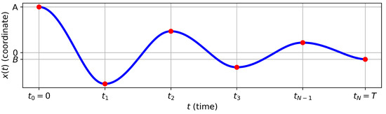
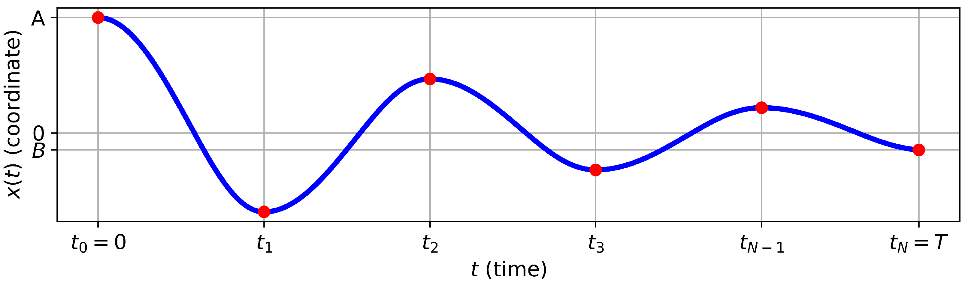
With any permissible control $\omega \left(t\right)$, it is observed that the trajectory $x\left(t\right)$ of the controlled system in (2) oscillates around the starting coordinate with successive intervals of monotonic increase and decrease (Figure 1). The amplitude and duration of each oscillation can vary, based on the chosen control function $\omega \left(t\right)$ (typically discontinuous). Indeed, if the conditions $\dot{x}\left(t_{*}\right)=0$ and $x\left(t_{*}\right)\ne 0$ are satisfied at some moment in time $t_{*}\in [0,T]$, it can be derived from the differential equation of problem (2) that $\ddot{x}\left(t\right)=-\mathsf{\mu }\dot{x}\left(t\right)-{\omega }^2\left(t\right)x\left(t\right)$. Given that the functions $x\left(t\right)$ and $\dot{x}\left(t\right)$ are continuous, the sign of the second derivative will match the sign of $x\left(t\right)$ in a small vicinity of point $t_{*}$, except, possibly, at a finite number of discontinuity points of the function $\omega \left(t\right)$. This implies that, for $x\left(t_{*}\right)>0$, the trajectory will have a point of local maximum, and, for $x\left(t_{*}\right)<0$, a point of local minimum.

Figure 1. An example of the trajectory of the controlled system (2) under the action of bang–bang control $\omega \left(t\right)$ for the case $\mathsf{\mu }=0.05$, ${\omega }_0=0.75$.

From the boundary conditions, it is understood that the speeds $\dot{x}\left(0\right)$ and $\dot{x}\left(T\right)$ at the initial and final moments of time equal zero, a situation that occurs only at the extreme points of the oscillatory process. These moments in time are denoted as $t_i$ (Figure 1), and the time intervals $t\in [t_i,t_{i+1}]$ are referred to as semi-oscillations. From this point, it is inferred that the optimal trajectory comprises a whole number of semi-oscillations N, being an even number when $B>0$, and an odd number when $B<0$ $(A>0)$.

To investigate the total optimal control problem, let us divide the trajectory into separate semi-oscillations and first solve the problem for one semi-oscillation $t\in [t_i,t_{i+1}]$. We will denote $A_i=x\left(t_i\right)$ ($A_0=A$, $A_N=B$). It leads to the following N subproblems for $i=0,\dots ,N-1$:

$$\left\{\begin{array}{c}\ddot{x}\left(t\right)+\mathsf{\mu }\dot{x}\left(t\right)+{\omega }^2\left(t\right)x\left(t\right)=0,t\in [t_i,t_{i+1}],\hfill \\ x\left(t_i\right)=A_i,\dot{x}\left(t_i\right)=0,\hfill \\ x\left(t_{i+1}\right)=A_{i+1},\dot{x}\left(t_{i+1}\right)=0,\hfill \\ t_{i+1}-t_i\to \underset{\omega \left(t\right)}{min}.\hfill \end{array}\right.$$

(3)

Utilizing the linearity and homogeneity of the differential equation allows for the normalization of the variable $x\left(t\right)$ by dividing it by its initial value $A_i$. It is also taken into account that the coefficient of friction $\mathsf{\mu }$ is independent of time t, meaning the initial moment in time can be considered as zero. This approach transforms all subproblems (3) for $i=0,\dots ,N-1$ into a unified auxiliary mini-problem of optimal control:

$$\left\{\begin{array}{c}{\ddot{x}}_i\left(t\right)+\mathsf{\mu }{\dot{x}}_i\left(t\right)+{\omega }_i^2\left(t\right)x_i\left(t\right)=0,t\in [0,T_i],\hfill \\ x_i\left(0\right)=1,{\dot{x}}_i\left(0\right)=0,\hfill \\ x_i\left(T_i\right)=A_{i+1}/A_i,{\dot{x}}_i\left(T_i\right)=0,\hfill \\ T_i\to \underset{{\omega }_i\left(t\right)}{min}.\hfill \end{array}\right.$$

(4)

Given probem (2) and knowing the numbers $t_i$ and $A_i$, the equation for optimal time in task (4) will be accurately represented by $T_i=t_{i+1}-t_i$, and the optimal trajectories and control in the auxiliary task (4) will coincide with the optimal trajectories and control in task (2) over the interval $[t_i,t_{i+1}]$ [1]. It will be demonstrated below that the optimal process is broken down into individual equal time intervals, calculated using analytical formulas.

Furthermore, for convenience in solving (4), instead of $x_i$ and ${\omega }_i$, the notations x and $\omega$ will be used.

4. Solution of the Optimal Control Problem for a Single Semi-Oscillation

In the previous section, it was demonstrated how to resolve the initial problem (2) by first solving an auxiliary problem:

$$\left\{\begin{array}{c}\ddot{x}\left(t\right)+\mathsf{\mu }\dot{x}\left(t\right)+{\omega }^2\left(t\right)x\left(t\right)=0,\hfill \\ x\left(0\right)=1,\dot{x}\left(0\right)=0,\hfill \\ x\left(T\right)=C<0,\dot{x}\left(T\right)=0,\hfill \\ \dot{x}\left(t\right)<0,t\in (0,T),\hfill \\ T\to \underset{\omega \left(t\right)}{min},\hfill \end{array}\right.$$

(5)

and find the dependency of the optimal time T on the terminal value C.

Here, the condition $\dot{x}\left(t\right)<0$ denotes the monotonicity of the trajectory $x\left(t\right)$, which corresponds to one semi-oscillation.

First, the question of controllability will be examined, and the range of values for C for which problem (5) has a solution will be defined.

The following notations will be introduced:

$${\beta }_1=\sqrt{1-\frac{{\mathsf{\mu }}^2}{4}},{\beta }_2=\sqrt{{\omega }_0^2-\frac{{\mathsf{\mu }}^2}{4}},$$

$${\phi }_1=arctan\left(\frac{2{\beta }_1}{\mathsf{\mu }}\right),{\phi }_2=arctan\left(\frac{2{\beta }_2}{\mathsf{\mu }}\right),$$

The largest value $x_{max}=\left|x\left(T\right)\right|$ can be attained with the control

$$\omega \left(t\right)=\left\{\begin{array}{c}1,x\left(t\right)>0,\hfill \\ {\omega }_0,x\left(t\right)\le 0,\hfill \end{array}\right.$$

(6)

because, with such control, acceleration is maximized when $x\left(t\right)\ge 0$ and deceleration is minimized when $x\left(t\right)<0$.

Similarly, the smallest value $x_{min}=\left|x\left(T\right)\right|$ can be reached analogously with the control

$$\omega \left(t\right)=\left\{\begin{array}{c}{\omega }_0,x\left(t\right)>0,\hfill \\ 1,x\left(t\right)\le 0.\hfill \end{array}\right.$$

(7)

Solving the differential equation with the boundary conditions from system (5) and with control (6) or (7), the following is obtained:

$$x_{min}\le \left|x\left(T\right)\right|\le x_{max},$$

(8)

where

$$x_{min}={\omega }_0{e}^{-\frac{\mathsf{\mu }}{2}\left(\frac{\pi -{\phi }_2}{{\beta }_2}+\frac{{\phi }_1}{{\beta }_1}\right)},x_{max}=\frac{1}{{\omega }_0}{e}^{-\frac{\mathsf{\mu }}{2}\left(\frac{\pi -{\phi }_1}{{\beta }_1}+\frac{{\phi }_2}{{\beta }_2}\right)}.$$

(9)

To apply PMP [1], we introduce the notation $\dot{x}\left(t\right)=v\left(t\right)$ and rewrite (5) in the form of a system of first-order differential equations:

$$\left\{\begin{array}{c}\dot{x}\left(t\right)=v\left(t\right),\hfill \\ \dot{v}\left(t\right)=-\mathsf{\mu }v\left(t\right)-{\omega }^2\left(t\right)x\left(t\right),\hfill \\ x\left(0\right)=1,v\left(0\right)=0,\hfill \\ x\left(T\right)=C<0,v\left(T\right)=0,\hfill \\ v\left(t\right)<0,t\in (0,T),\hfill \\ T\to \underset{\omega \left(t\right)}{min}.\hfill \end{array}\right.$$

(10)

Now, we let the terminal value C satisfy condition (8), which ensures the controllability of the system.

We write the Pontryagin function:

$$H({\psi }_1,{\psi }_2,x,v,\omega )={\psi }_{1}vs.-{\psi }_2(\mathsf{\mu }vs.+{\omega }^{2}x)$$

and denote its upper boundary:

$$M({\psi }_1,{\psi }_2,x,v)=\underset{\omega \in [{\omega }_0,1]}{sup}H({\psi }_1,{\psi }_2,x,v,\omega )$$

If $x\left(t\right)$, $v\left(t\right)$, and $\omega \left(t\right)$ constitute a solution to the optimal control problem (10), then the following three conditions are satisfied:

(I)

There exist continuous functions ${\psi }_1\left(t\right)$ and ${\psi }_2\left(t\right)$, which never simultaneously become zero and are solutions to the adjoint system:

$$\left\{\begin{array}{c}{\dot{\psi }}_1\left(t\right)=-\frac{\partial H}{\partial x}={\psi }_2\left(t\right){\omega }^2\left(t\right),\hfill \\ {\dot{\psi }}_2\left(t\right)=-\frac{\partial H}{\partial v}=-{\psi }_1\left(t\right)+\mathsf{\mu }{\psi }_2\left(t\right).\hfill \end{array}\right.$$

(11)

(II)

For any $t\in [0,T]$, the maximum condition is satisfied:

$$H({\psi }_1\left(t\right),{\psi }_2\left(t\right),x\left(t\right),v\left(t\right),\omega \left(t\right))=M({\psi }_1\left(t\right),{\psi }_2\left(t\right),x\left(t\right),v\left(t\right)).$$

(12)

(III)

For any $t\in [0,T]$, a specific inequality occurs:

$$M({\psi }_1\left(t\right),{\psi }_2\left(t\right),x\left(t\right),v\left(t\right))\ge 0.$$

From condition (12) for the maximum of the function H, the optimal control is obtained in the form

$$\omega \left(t\right)=\left\{\begin{array}{c}1,{\psi }_2\left(t\right)x\left(t\right)<0,\hfill \\ {\omega }_0,{\psi }_2\left(t\right)x\left(t\right)>0,\hfill \\ \mathrm{unknown}\mathrm{value},{\psi }_2\left(t\right)x\left(t\right)\equiv 0.\hfill \end{array}\right.$$

(13)

Let us show that the case of singular control in Formula (13), specifically when ${\psi }_2\left(t\right)x\left(t\right)\equiv 0$ over a non-zero length interval of time, is impossible, assuming the opposite. This means considering the existence of a time interval during which ${\psi }_2\left(t\right)x\left(t\right)\equiv 0$. In such an interval, determining the value of optimal control from the maximum condition would not be feasible.

Given the continuity of the functions ${\psi }_2\left(t\right)$ and $x\left(t\right)$, it is possible either for ${\psi }_2\left(t\right)\equiv 0$ over some interval or for $x\left(t\right)\equiv 0$ over a certain time period.

If ${\psi }_2\left(t\right)\equiv 0$, then ${\dot{\psi }}_2\left(t\right)\equiv 0$ must also be, identically, zero. However, this conclusion, derived from the second equation of the adjoint system (11), implies that ${\psi }_1\left(t\right)\equiv 0$, contradicting the maximum principle’s condition (I).

In the scenario where $x\left(t\right)\equiv 0$, it follows that $v\left(t\right)=\dot{x}\left(t\right)\equiv 0$. Such a case is deemed impossible, as the controlled system cannot stay in a zero state under any control value, given that the term of the system’s differential Equation (5), which includes the control, would also equate to zero.

This reasoning leads to the formulation of a statement:

Lemma 1. 

Optimal control $\omega \left(t\right)$ is limited to only two values, 1 and ${\omega }_0$, dictated by the sign of the product ${\psi }_2\left(t\right)x\left(t\right)$. Considering the case where this product equals zero as non-existent is justified by the fact that the control value at a single point or a finite number of points lacks any impact on the trajectory of the controlled system.

Now, we consider condition (III). It represents the greatest interest at values $t=0$ and $t=T$.

At $t=0$, the condition is expressed as

$$\begin{array}{c}\hfill M({\psi }_1\left(0\right),{\psi }_2\left(0\right),x\left(0\right),v\left(0\right))=H({\psi }_1\left(0\right),{\psi }_2\left(0\right),x\left(0\right),v\left(0\right),\omega \left(0\right))={\psi }_1\left(0\right)v\left(0\right)-{\psi }_2\left(0\right)(\mathsf{\mu }v\left(0\right)+{\omega }^2\left(0\right)x\left(0\right))\ge 0.\end{array}$$

(14)

At $t=T$, the condition becomes

$$\begin{array}{c}\hfill M({\psi }_1\left(T\right),{\psi }_2\left(T\right),x\left(T\right),v\left(T\right))=H({\psi }_1\left(T\right),{\psi }_2\left(T\right),x\left(T\right),v\left(T\right),\omega \left(T\right))={\psi }_1\left(T\right)v\left(T\right)-{\psi }_2\left(T\right)(\mathsf{\mu }v\left(T\right)+{\omega }^2\left(T\right)x\left(T\right))\ge 0.\end{array}$$

(15)

Given the boundary conditions that $v\left(0\right)=v\left(T\right)=0$, and considering that the control value $\omega \left(t\right)$ is always positive, with $x\left(0\right)>0$ and $x\left(T\right)<0$, the following additional conditions are derived from (14) and (15)

$${\psi }_2\left(0\right)\le 0,{\psi }_2\left(T\right)\ge 0.$$

(16)

Now, we explore the potential form of optimal control and the number of switches. It is already known that the value of optimal control is determined by the sign of the product ${\psi }_2\left(t\right)x\left(t\right)$.

The trajectory $x\left(t\right)$, due to its monotonic nature, crosses zero only once. This moment in time is denoted as $\tau$.

Thus, control $\omega \left(t\right)$ may only change its value at the point $\tau$ and at points where the sign of the adjoint variable ${\psi }_2\left(t\right)$ changes. If at point $\tau$, both $x\left(t\right)$ and ${\psi }_2\left(t\right)$ change their signs simultaneously, then the control value remains unchanged.

Firstly, consider an interval of time where control $\omega \left(t\right)\equiv 1$. Then, the general solution $x\left(t\right)$ of the differential equation from system (4) and ${\psi }_2\left(t\right)$ from the adjoint system (5) will take a specific form:

$$x\left(t\right)=e^{-\frac{\mathsf{\mu }}{2}t}{C}_{1}sin({\beta }_{1}t+C_2),{\psi }_2\left(t\right)=e^{\frac{\mathsf{\mu }}{2}t}{C}_{3}sin({\beta }_{1}t+C_4),$$

(17)

where constants $C_1$, $C_2$, $C_3$, and $C_4$ must be determined from the boundary conditions on the interval of constant control. The value of the adjoint variable ${\psi }_1\left(t\right)$ is not of interest, as it does not enter into Formula (13).

Now, we consider an interval of time during which control $\omega \left(t\right)\equiv {\omega }_0$. Similarly, it is obtained that

$$x\left(t\right)=e^{-\frac{\mathsf{\mu }}{2}t}{D}_{1}sin({\beta }_{2}t+D_2),{\psi }_2\left(t\right)=e^{\frac{\mathsf{\mu }}{2}t}{D}_{3}sin({\beta }_{2}t+D_4),$$

(18)

where constants $D_1$, $D_2$, $D_3$, and $D_4$ are also to be determined from the boundary conditions.

It is now proposed that the adjoint variable ${\psi }_2\left(t\right)$ turns to zero at most twice within the interval $[0,\tau ]$, or in $[\tau ,T]$. For instance, let ${\psi }_2\left({\xi }_1\right)={\psi }_2\left({\xi }_2\right)=0$, where $0\le {\xi }_1<{\xi }_2\le \tau$. Then, within the interval $[{\xi }_1,{\xi }_1]$, the control value does not change, and this leads to a contradiction with Formulas (17) and (18) because the distance between zeros of the function ${\psi }_2\left(t\right)$ (for example, $\frac{\pi }{{\beta }_1}$ for Formula (17)) exceeds the maximum length of an interval of constancy of sign and monotonicity of the function $x\left(t\right)$ (for example, $\frac{\pi -{\phi }_1}{{\beta }_1}$ or $\frac{{\phi }_1}{{\beta }_1}$).

Thus, it is proven that

Lemma 2. 

In problem 5, optimal control can have no more than one switch in each of the intervals $[0,\tau ]$ and $[\tau ,T].$

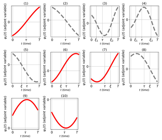
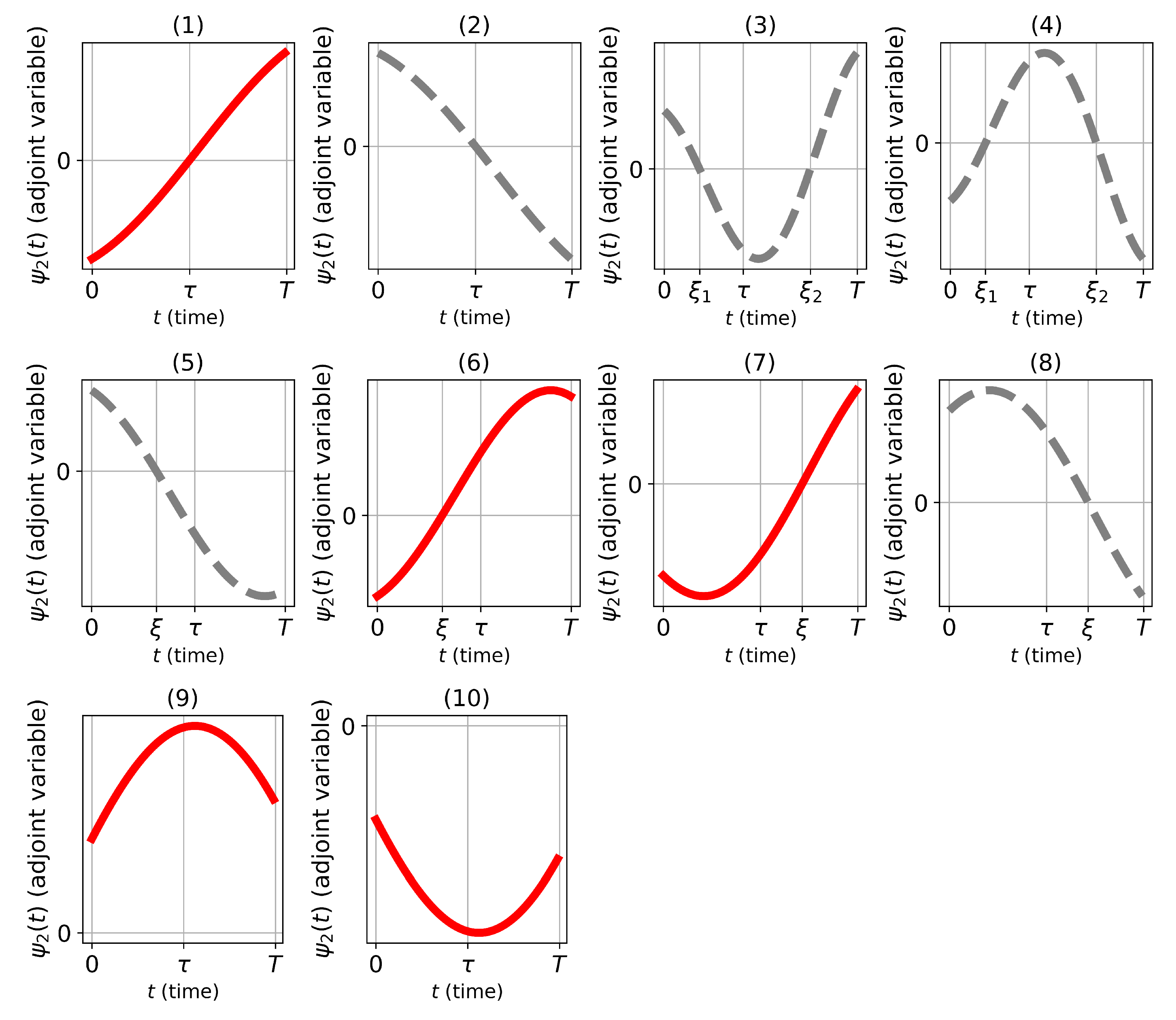
The function ${\psi }_2\left(t\right)$ has a continuous derivative (as the right-hand side of the second equation of the adjoint system (11) is continuous) and turns to zero no more than twice within the interval $[0,T]$. Moreover, these zeros cannot both lie within the same subinterval $[0,\tau ]$ or $[\tau ,T]$. This leads to 10 different cases (Figure 2) of sign changes for the function ${\psi }_2\left(t\right)$ over the interval $[0,T]$. Dashed gray lines on the graph indicate scenarios that contradict the PMP, while solid red lines indicate cases with no contradiction with PMP found. A detailed analysis of these cases is provided.

Figure 2. Cases (1)–(10) of sign changes in the function ${\psi }_2\left(t\right)$. The dashed gray line represents situations that do not satisfy the PMP. The solid red line represents cases that do not contradict the PMP.

If ${\psi }_2\left(\tau \right)=0$, then ${\psi }_2\left(t\right)\ne 0$ for $t\ne \tau$, leading to cases (1) and (2). In case (1), a constant control equal to 1 is maintained throughout the entire time interval. Case (2) is not possible, as ${\psi }_2\left(T\right)<0$ and does not satisfy condition (16).

If ${\psi }_2\left(t\right)$ turns to zero twice within the interval $(0,T)$, there exist ${\xi }_1\in (0,\tau )$ and ${\xi }_2\in (\tau ,T)$ such that ${\psi }_2\left({\xi }_1\right)=0$ and ${\psi }_2\left({\xi }_2\right)=0$, leading to cases (3) and (4). These cases contradict condition (16) since ${\psi }_2\left(0\right)$ and ${\psi }_2\left(T\right)$ have the same sign.

If ${\psi }_2\left(t\right)$ turns to zero once at a point $\xi \in (0,\tau )$ and does not equal zero within the interval $(\tau ,T)$, cases (5) and (6) are obtained. Case (5) is impossible because ${\psi }_2\left(0\right)>0$.

If ${\psi }_2\left(t\right)$ turns to zero once at a point $\xi \in (\tau ,T)$ and does not equal zero within the interval $(0,\tau )$, cases (7) and (8) emerge. Case (8) is not feasible, as ${\psi }_2\left(T\right)<0$.

Finally, if ${\psi }_2\left(t\right)$ does not turn to zero within the interval $(0,T)$, cases (9) and (10) are considered. Case (9) is possible if ${\psi }_2\left(0\right)=0$. Case (10) is possible if ${\psi }_2\left(T\right)=0$.

After analyzing cases (1–10), it is determined that the following statement holds:

Lemma 3. 

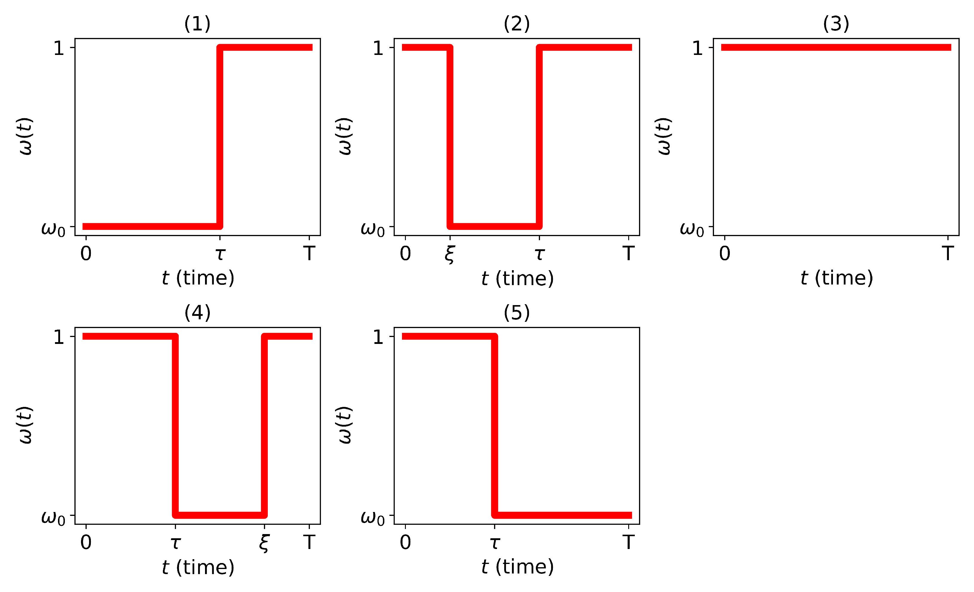
Optimal control (bang–bang) in the problem (5) can be one of the five types represented in Figure 3.

Figure 3. All possible variants of optimal control encountered in problem (10).

It is noted that all types of control satisfying the maximum principle (illustrated in Figure 3) differ in the length of the segment where the control value equals ${\omega }_0$, and its placement, respectively, to the point $\tau$.

Introducing the parameter $s=\xi -\tau$, the values of $\tau$ and T can be distinctly determined from the equation and three boundary conditions (excluding the condition $x\left(T\right)=C$) of problem (5) by substituting the corresponding control. This results in the determination of the end time $T\left(s\right)$ and the terminal value $C\left(s\right)=x\left(T\right(s\left)\right)$ as functions of the unknown parameter s.

For control type 3 (illustrated in Figure 3), $s=0$ corresponds, and for control type 1, the smallest value $s_{min}=-\frac{\pi -{\phi }_2}{{\beta }_2}<0$. For control type 5, the largest value $s_{max}=\frac{{\phi }_2}{{\beta }_2}$ is obtained as the longest possible duration of motion under constant control $\omega \left(t\right)\equiv {\omega }_0$, that is $s_{max}=T-\tau$, with the moments of time $\tau$ and T derived from Formula (18) and the conditions $x\left(\tau \right)=0$, $\dot{x}\left(T\right)=0$, $x\left(T\right)<0$, $T>\tau$, aiming to minimize $T-\tau$. Similarly, from Formula (18), the smallest value of $s_{\min }=-\tau$ is obtained. Controls of type 2 and 4 correspond to intermediate values of s within intervals $(s_{min},0)$ and $(0,s_{max})$.

Knowing the switching moment of control and having an analytical solution (Formulas (17) and (18)), the end time T and the terminal trajectory value $x\left(T\right)$ can be explicitly calculated as functions of the parameter s.

Let us consider $s\in \left[0,\frac{{\phi }_2}{{\beta }_2}\right]$; then, for $t\in [0,\tau )$, $\omega \left(t\right)\equiv 1$ and from Formula (17) and the initial condition $x\left(0\right)=1,\dot{x}\left(0\right)=0$, it is found that $C_1=\frac{1}{{\beta }_1}$, $C_2={\phi }_1$, leading to $x\left(t\right)=\frac{1}{{\beta }_1}{e}^{-\frac{\mathsf{\mu }}{2}t}sin({\beta }_{1}t+{\phi }_1)$ and $\tau =\frac{\pi -{\phi }_1}{{\beta }_1}$.

Subsequently, for $t\in [\tau ,\tau +s)$, $\omega \left(t\right)\equiv {\omega }_0$ and from Formula (18) and the continuity of $\dot{x}\left(t\right)$ at $t=\tau$, similarly, $x\left(t\right)=-\frac{1}{{\beta }_2}{e}^{-\frac{\mathsf{\mu }}{2}t}sin\left({\beta }_2(t-\tau )\right)$.

Finally, for $t\in [\tau +s,T]$, $\omega \left(t\right)\equiv 1$ and from Formula (17) and the continuity of $\dot{x}\left(t\right)$ at $t=\tau +s$, it is found that

$$x\left(t\right)=-\frac{e^{-\frac{\mathsf{\mu }}{2}t}sin\left({\beta }_{2}s\right)sin({\beta }_1(t-\tau -s)+{\phi }_3)}{{\beta }_{2}sin\left({\phi }_3\right)},$$

(19)

where ${\phi }_3=arctan\left(\frac{{\beta }_1}{{\beta }_2}tan\left({\beta }_{2}s\right)\right)$.

From Formula (19) and the condition $\dot{x}\left(T\right)=0$, the end moment of time is obtained as follows:

$$T\left(s\right)=\frac{1}{{\beta }_1}(\pi -{\phi }_3)+s.$$

(20)

Simplifying Expressions (19) and (20), ultimately, for $s\in [0,s_{max}]$, one obtains

$$\begin{array}{c}T\left(s\right)=\frac{1}{{\beta }_1}\left(\pi -arctan\left(\frac{{\beta }_1}{{\beta }_2}tan\left({\beta }_{2}s\right)\right)\right)+s,\hfill \\ \\ C\left(s\right)=x\left(T\left(s\right)\right)=-\frac{1}{{\beta }_2}{e}^{-\frac{\mathsf{\mu }}{2}T\left(s\right)}\sqrt{{\beta }_2^2{cos}^2\left({\beta }_{2}s\right)+{\beta }_1^2{sin}^2\left({\beta }_{2}s\right)}.\hfill \end{array}$$

(21)

Conducting analogous calculations for the case $s\in \left[s_{min},0\right)$, one obtains

$$\begin{array}{c}T\left(s\right)=\frac{1}{{\beta }_1}\left(\frac{\pi }{2}-arctan\left(\frac{{\beta }_2}{{\beta }_1}cot\left({\beta }_{2}s\right)\right)\right)-s,\hfill \\ \\ C\left(s\right)=\frac{-{\beta }_2{e}^{-\frac{\mathsf{\mu }}{2}T\left(s\right)}}{\sqrt{{\beta }_2^2{cos}^2\left({\beta }_{2}s\right)+{\beta }_1^2{sin}^2\left({\beta }_{2}s\right)}}.\hfill \end{array}$$

(22)

We note that Formulas (21) and (22) parametrically define a certain curve $T\left(C\right)$ depicting the dependency of the end time on the terminal value C when utilizing controls that satisfy the maximum principle. The parametric formulation of the function allows for the calculation of the first two derivatives of $T\left(C\right)$ as functions of the variable C. Thus, the following properties of the function $T\left(C\right)$ are established

Lemma 4. 

Formulas (21) and (22):

1.

Uniquely determine the function $T\left(C\right)$, defined for $C\in [-x_{max},-x_{min}]$.

2.

The function $T\left(C\right)$ is continuous for $C\in [-x_{max},-x_{min}]$.

3.

The function $T\left(C\right)$ is differentiable for $C\in (-x_{max},-x_{min})$. At the endpoints of the interval, the derivative equals infinity, while at the point corresponding to the parameter $s=0$, the derivative equals zero. Let $x_{*}=-C\left(0\right)$ be denoted.

4.

The function $T\left(C\right)$ decreases on the interval $C\in [-x_{max},-x_{*}]$ and increases on the interval $C\in [-x_{*},-x_{min}]$.

5.

The second derivative of the function $T\left(C\right)$ is negative on the intervals $C\in (-x_{max},-x_{*})\cup (-x_{*},-x_{min})$. This condition signifies that the function $T\left(C\right)$ is concave down for $C\in [-x_{max},-x_{min}]$.

Remark 1. 

It is important to note that the constancy of the sign of the second derivative was established by calculations via symbolic mathematics by Wolfram.

Investigating the properties of the function $T\left(C\right)$, it was found that each permissible terminal value C corresponds to a unique control that satisfies the PMP. Therefore, the statement follows

Lemma 5. 

The function $T\left(C\right)$, defined by formulas (21) and (22), determines the optimal time in problem (5).

Example 1

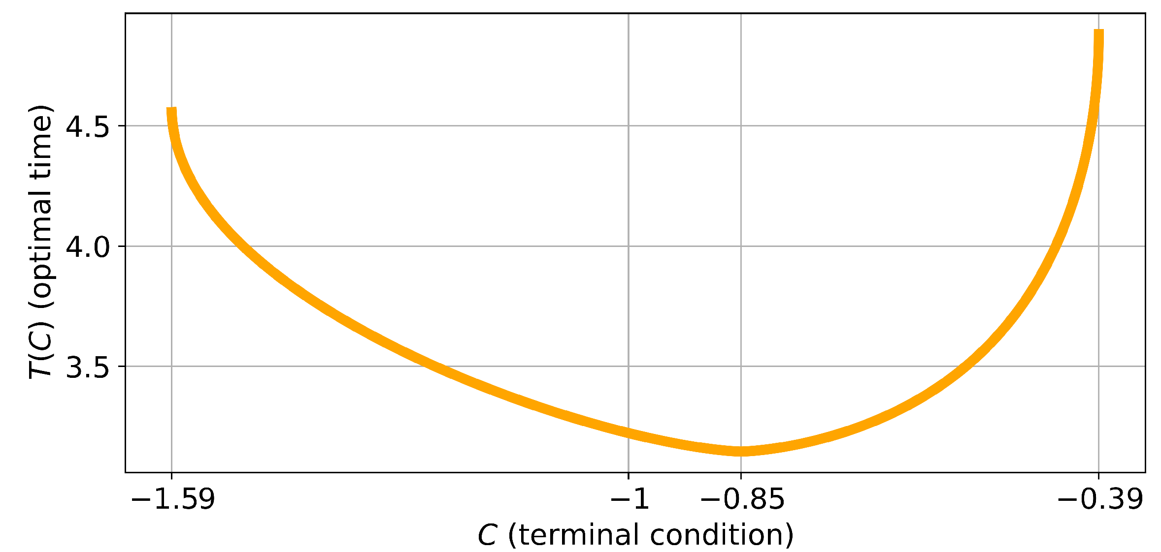
Considering an example with given parameters $\mathsf{\mu }=0.1$, ${\omega }_0=0.5$, it is calculated that $x_{min}\approx 0.39$, and $x_{max}\approx 1.59$. From (21), it is found that $x_{*}=C\left(0\right)\approx 0.85$. Figure 4 illustrates the graph of the function $T\left(C\right)$, demonstrating how the optimal time varies with different terminal values C within the specified range.

Figure 4. Optimal time curve $T\left(C\right)$ in problem (5) for the case of $\mathsf{\mu }=0.1$, ${\omega }_0=0.5$.

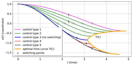
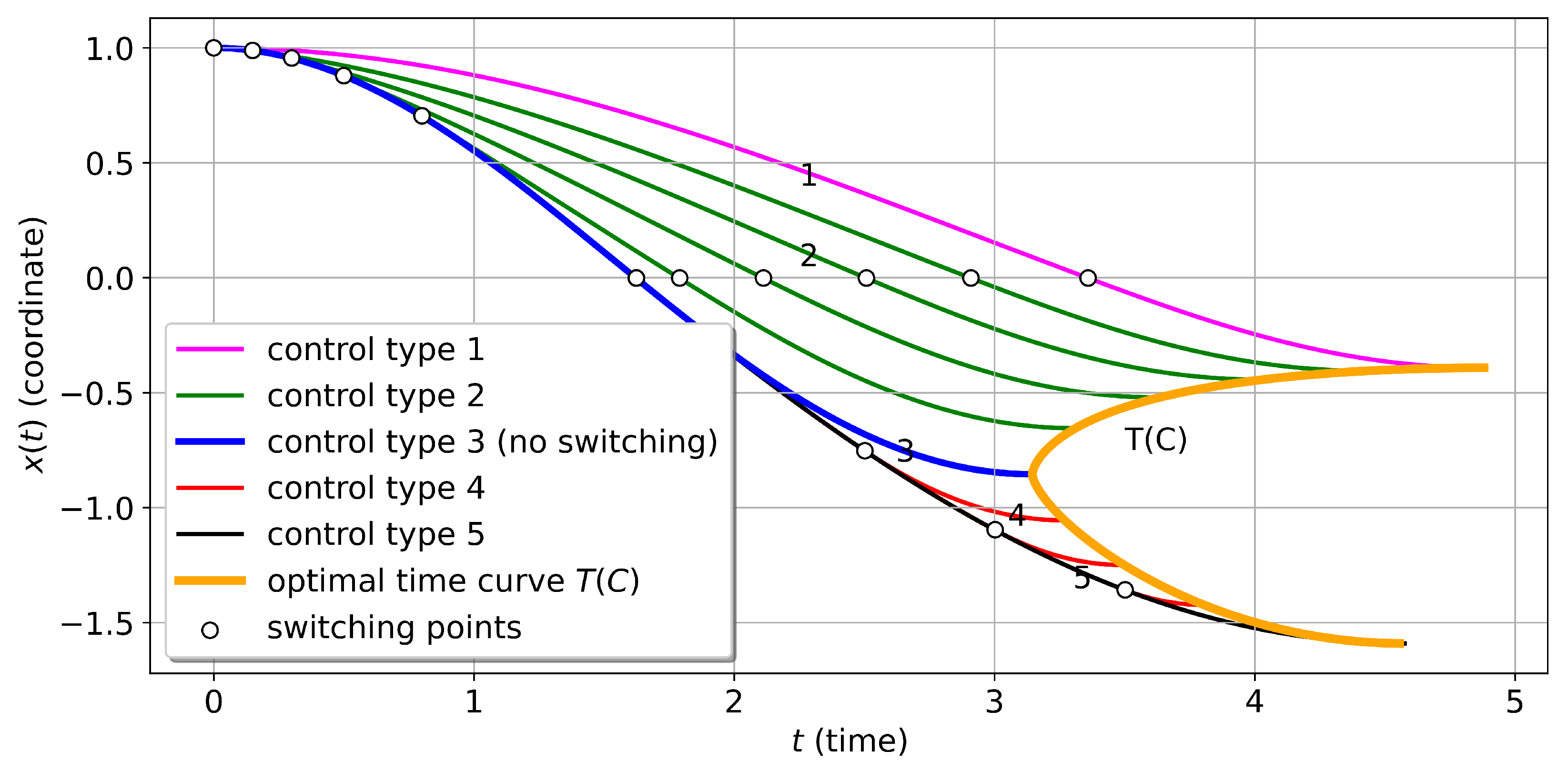
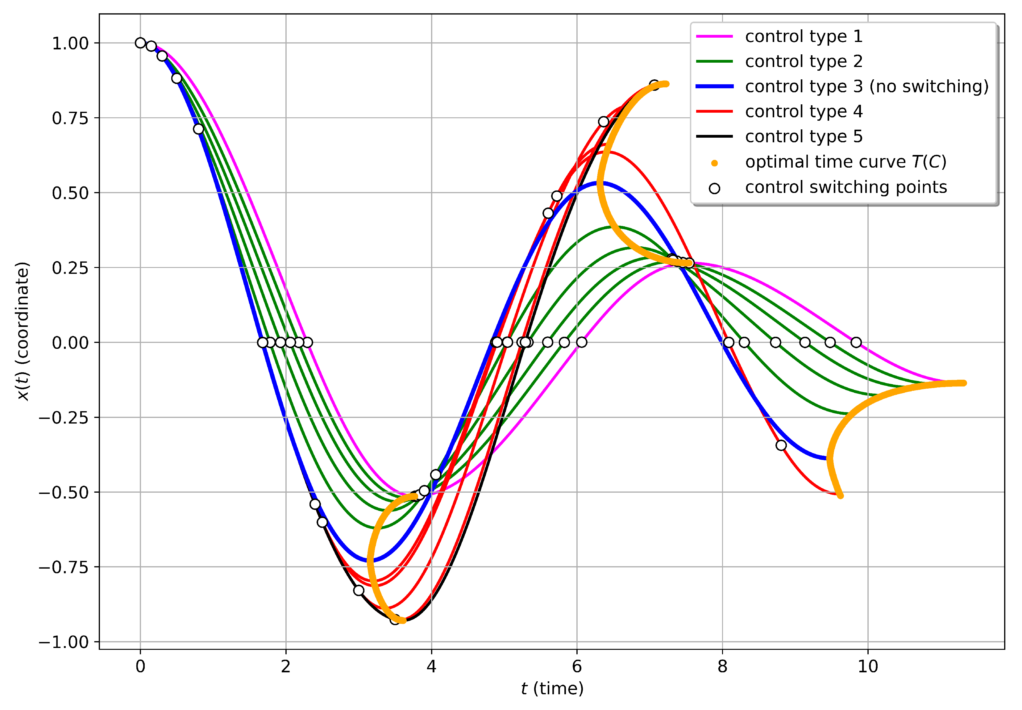
It has been demonstrated that each value of s unequivocally corresponds to a specific optimal control and an optimal trajectory, leading to a particular terminal point $C\left(s\right)$. Different optimal trajectories, corresponding to various types of controls, are presented in Figure 5. Controls of types 1 and 5 correspond to trajectories reaching the extreme points of the reachability set. Control of type 2 corresponds to the upper branch of the $T\left(C\right)$ curve (left branch on Figure 4). Control of type 3, which has no switches, corresponds to the trajectory with the minimum possible time. Control of type 4 corresponds to the lower branch of the $T\left(C\right)$ curve (right branch on Figure 4).

Figure 5. The reachability set of optimal trajectories and control switching points for various values of C in the case of a single oscillation. $\mathsf{\mu }=0.1$, ${\omega }_0=0.5$.

Trajectories are constructed for the given parameter values on Figure 4, but the general character of the drawing does not change with different parameter values.

5. Solution to the General Timing Optimal Problem

We apply the results of the previous section to solve the original problem (2). Let us first explore the question of controllability and determine under what boundary conditions A and B the system is controllable.

Using the estimate (8), we obtain an estimate for $x\left(T\right)$ depending on the number of semi-oscillations N:

$$A{x}_{min}^N\le \left|x\left(T\right)\right|\le A{x}_{max}^N.$$

(23)

Thus, the lemma is the following:

Lemma 6. 

The system is controllable if and only if there exists an even natural number N (for $B>0$) or an odd natural number N (for $B<0$), such that

$$\left|\frac{B}{A}\right|\in [x_{min}^N,x_{max}^N].$$

(24)

Since ${\phi }_2\in (0,\pi /2)$ and ${\omega }_0<1$, it follows that $x_{min}<1$ and $x_{min}^N\to 0$ as $N\to +\infty$.

Therefore, the system will be controllable for any non-zero values of A and B provided that

$$x_{max}>1.$$

Utilizing Formula (9), this inequality can be expressed as follows:

$$-\frac{\pi -arctan\left(\frac{\sqrt{4-{\mathsf{\mu }}^2}}{\mathsf{\mu }}\right)}{\frac{\sqrt{4-{\mathsf{\mu }}^2}}{\mathsf{\mu }}}+\frac{arctan\left(\frac{\sqrt{4{\omega }_0^2-{\mathsf{\mu }}^2}}{\mathsf{\mu }}\right)}{\frac{\sqrt{4{\omega }_0^2-{\mathsf{\mu }}^2}}{\mathsf{\mu }}}>ln{\omega }_0.$$

(25)

Having resolved the question of controllability, we now return to the original problem of optimal control (2). Given $x\left(t\right)$, the solution of the optimal control problem (2), let us consider two consecutive semi-oscillations $t\in [t_{i-1},t_{i+1}]$. This segment of the optimal trajectory satisfies the boundary conditions of the original problem and must itself be optimal. Using the results of the previous section and normalizing variable $x\left(t\right)$, the time for this segment can be expressed by the formula

$$t_{i+1}-t_{i-1}=T\left(\frac{x\left(t_{i+1}\right)}{x\left(t_i\right)}\right)+T\left(\frac{x\left(t_i\right)}{x\left(t_{i-1}\right)}\right)=T\left(\frac{A_{i+1}}{A_i}\right)+T\left(\frac{A_i}{A_{i-1}}\right).$$

We fix $A_{i+1}$ and $A_{i-1}$ (noting that they have the same sign) and find the minimum of the last expression by the variable $A_i$. Denoting $D=\frac{A_{i+1}}{A_{i-1}}$ and introducing a new variable $q=\frac{A_i}{A_{i-1}}$, the time $t_{i+1}-t_{i-1}$ can be expressed by the function

$$g\left(q\right)=t_{i+1}-t_{i-1}=T\left(q\right)+T\left(\frac{D}{q}\right),$$

where $T\left(C\right)$ is parametrically defined using Formulas (21) and (22). Let q and $\frac{D}{q}$ belong to the domain of definition of the function $T\left(C\right)$. We find the first derivative of the function $g\left(q\right)$:

$$g^{\prime }\left(q\right)=T^{\prime }\left(q\right)-T^{\prime }\left(\frac{D}{q}\right)\frac{D}{q^2}.$$

It is easy to notice that this derivative becomes zero at the point $q_{*}=-\sqrt{D}$. Let us compute the second derivative at the point $q_{*}$:

$$\begin{array}{c}\hfill g^{″}\left(q_{*}\right)=T^{″}\left(q_{*}\right)+T^{″}\left(\frac{D}{q_{*}}\right)\frac{D^2}{q_{*}^4}+T^{\prime }\left(\frac{D}{q_{*}}\right)\frac{2D}{q_{*}^3}=2T^{″}(-\sqrt{D})-T^{\prime }\left(-\sqrt{D}\right)\frac{2}{\sqrt{D}}.\end{array}$$

(26)

Given that $-\sqrt{D}\in (-x_{max},-x_0]$, the function $T\left(C\right)$ decreases and is concave downwards. Therefore, all terms in the above expression are positive, and the found point is a point of minimum. At the boundary points of the domain of definition, the function $T\left(C\right)$ is not differentiable, but, in this case, there exists a unique control (either Equations (6) or (7)), leading the controlled system to its extreme position. For the remaining values of $-\sqrt{D}$, the positivity of the above expression (26) follows from complex algebraic manipulations using the parametric setting of the function $T\left(C\right)$ with the help of Formulas (21) and (22).

We have shown that the numbers $A_{i-1}$, $A_i$, and $A_{i+1}$ form a geometric progression. Applying this reasoning to the entire trajectory, we obtain the following statement:

Lemma 7. 

The numbers $A_i$ for the optimal process satisfy the condition

$$A_i=A{\left(-\sqrt[N]{\frac{\left|B\right|}{A}}\right)}^i,i=0,\dots ,N,$$

where the number of semi-oscillations is determined as the smallest N satisfying Lemma 6.

Since the ratio $\frac{A_{i+1}}{A_i}$ is constant for the optimal trajectory, the optimal control on each segment $[t_i,t_{i+1}]$ will be the same. Hence, if the number of semi-oscillations required to reach the end point is more than one, then the optimal control is a periodic function, where the period is one semi-oscillation.

6. Main Result

Thus, necessary and sufficient conditions are determined for the optimal control problem to have a solution. The controlled process is oscillatory in nature and a formula has been obtained to determine the number of semi-oscillations. It has been proven that the amplitudes of semi-oscillations form a geometric progression. We will combine all the statements proven above (Lemmas 1–7) into a step-by-step algorithm for solving the original problem (2).

• Determine if the problem has a solution and find the number of semi-oscillations N from the condition (24). Note that the problem will have a solution for any $A>0$ and $B\ne 0$ if condition (25) is satisfied.
• Calculate the denominator of the geometric progression $C_{*}=\frac{A_{i+1}}{A_i}$ using formula

  $$C_{*}=-\sqrt[N]{\frac{\left|B\right|}{A}}.$$

  (27)
  This value determines how much the amplitude changes over one semi-oscillation.
• Using the parametric setting (21) and (22) of the function $T\left(C\right)$ and the value $C_{*}$ found in the previous step, calculate the value of the parameter $s_{*}$ as the solution of the equation $C\left(s_{*}\right)=C_{*}$ and the duration of one semi-oscillation $T_{*}=T\left(C_{*}\right)$.
  The optimal time for rapid action in problem (2) is then

  $$T=N{T}_{*}.$$
• The value $s_{*}=\xi -\tau$ uniquely determines the type of optimal control for one semi-oscillation (Figure 3) and allows determining the number and position of switching points for one semi-oscillation.
  In the case of $s_{*}>0$ we have optimal control of the type 4 or 5. In this case, within one semi-oscillation, we calculate the moment of the first switching $\tau =\frac{\pi -{\phi }_1}{{\beta }_1}$. Then, if $s_{*}<s_{max}$, the second switching moment is calculated using formula $\xi =\tau +s_{*}$.
  In the case of $s_{*}=0$, there is no switching moment (it is optimal control of type 3).
  In the case of $s_{*}<0$, the optimal control of the type 1 or 2 is considered. Here, first, the second switching moment $\tau =T_{*}-\frac{{\phi }_1}{{\beta }_1}$ is calculated, then the first switching moment $\xi =\tau +s_{*}$ is found.
  Subsequently, control values for each semi-oscillation periodically repeat. Thus, we find the optimal control and optimal trajectory over the entire segment $t\in [0,T]$.

6.1. Example 2

Applying the obtained algorithm, we find the optimal control and trajectory for the parameter values $A=1$, $B=-\frac{1}{4}$, $\mathsf{\mu }=0.1$, and ${\omega }_0=0.5$.

From Equation (9), it follows that $x_{min}\approx 0.39$ and $x_{max}\approx 1.59$. From (21), $x_{*}=C\left(0\right)\approx 0.85$. It is also noted that, since $x_{max}>1$, the problem will have a solution for any boundary conditions given the specific values of $\mathsf{\mu }$ and ${\omega }_0$.

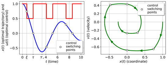
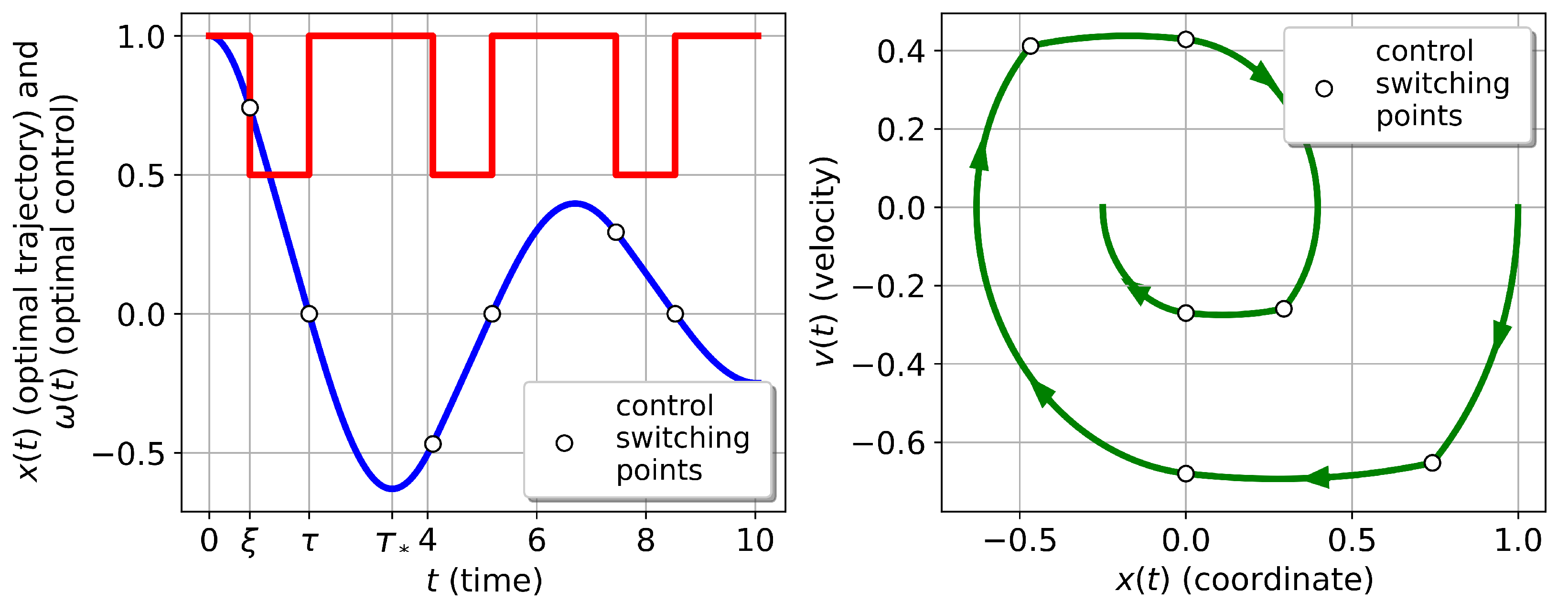
From (24), it is determined that the end point is reachable within $N=3$ semi-oscillations. Further, according to the Formula (27), the value is $C_{*}=-\sqrt[3]{\frac{1}{4}}\approx -0.63$. This value of $C_{*}$ corresponds to Formula (22) and optimal control of type 2, from which we find $s_{*}\approx -1.09$, $T_{*}\approx 3.35$, and $T=T_{*}·3\approx 10.05$. The second switching moment is $\tau \approx 1.83$ and the first switching moment is $\xi \approx 0.74$. The optimal trajectory and phase portrait are shown on Figure 6.

Figure 6. Optimal trajectory $x\left(t\right)$ (blue), control $\omega \left(t\right)$ (red), and phase portrait (green) for $\mathsf{\mu }=0.1$, ${\omega }_0=0.5$.

6.2. Example 3

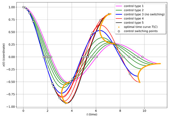
Using the obtained result about the periodicity of optimal control, we can construct the reachability set and optimal trajectories for the case when the endpoint is reachable within no more than three semi-oscillations for $\mathsf{\mu }=0.2$, ${\omega }_0=0.75$ (Figure 7). Since the optimal control is a periodic function, the optimal trajectories are first constructed for several selected values of the parameter s on one semi-oscillation using given above algorithm. Then, the optimal control on one semi-oscillation is repeated on the next two semi-oscillations. For this example, three semi-oscillations are considered, but the process could easily be extended to any number of semi-oscillations.

Figure 7. The reachability set of optimal trajectories and control switching points for various values of C in the case of no more than 3 semi-oscillations. $\mathsf{\mu }=0.2$, and ${\omega }_0=0.75$.

It is important to note the discontinuity in the curve of optimal time $T\left(C\right)$ in the case of more than one semi-oscillation. That is, a small change in the boundary conditions can lead to a significant change in the optimal time by increasing the number of semi-oscillations at the optimal trajectory. We also note that for these parameter values, condition (25) is not satisfied, and the optimal control problem is not solvable for any boundary conditions. Figure 7 shows that all optimal trajectories are damped oscillations and, although the optimal control is a periodic function, this period differs for different trajectories.

7. Conclusions

In conclusion, this study presents an insightful examination of a bilinear optimal control problem, with a particular emphasis on the coefficient modulation. Through rigorous analysis, it has been established that optimal control is non-singular, the optimal process exhibits periodic characteristics with oscillatory behavior, and the amplitudes form a geometric progression. Furthermore, it was determined that while the optimal process itself is indeed periodic, the control function does not retain symmetry within a single period.

The implications of these findings extend to the broader realm of control theory and its applications in engineering and physics, offering a new perspective on the nature of bilinear control systems. The periodicity of the optimal process suggests potential for efficient energy usage and system stabilization in various applications, from mechanical systems to electrical circuits.

However, the lack of symmetry in the control function within the period underscores the complexity of bilinear control systems and indicates that intuition alone may not be sufficient to predict the system behavior. Future research may explore the nuances of this asymmetry and its impact on system performance.

As far as zero speed boundary conditions are concerned, our study is focused on mechanisms that perform full oscillations. Therefore, we can always use such boundary conditions for the fastest damping.

The analytical solution obtained in the paper allows for the precise determination of the switching moments, as well as the amplitudes and the total optimal time of the process.This paper contributes to the ongoing discourse in control theory, providing a foundation for subsequent studies to build upon. The results underscore the necessity for a nuanced approach to control strategy development, especially in systems where time-optimality is a paramount consideration. The methodologies and findings herein have practical implications for designing more efficient and robust control systems in the future.

References

- Pontryagin, L.S.; Boltyanskii, V.G.; Gamkrelidze, R.V.; Mishchenko, E.F. The Mathematical Theory of Optimal Processes; Interscience Publishers (division of John Wiley and Sons, Inc.): New York, NY, USA, 1962; 360p. [Google Scholar]
- Lewis, F.L.; Vrabie, D.; Syrmos, V.L. Optimal Control; John Wiley and Sons, Inc.: Hoboken, NJ, USA, 2012; 540p. [Google Scholar]
- Kirk, D.E. Optimal Control Theory: An Introduction; Dover Publications, Inc.: New York, NY, USA, 2004; 464p. [Google Scholar]
- Bryson, A.E.; Ho, Y.C. Applied Optimal Control: Optimization, Estimation, and Control; Taylor & Francis Group: New York, NY, USA, 1975; 496p. [Google Scholar]
- Geradin, M.; Rixen, D. Mechanical Vibrations: Theory and Application to Structural Dynamics; John Wiley & Sons, Ltd: Chichester, UK, 2015; 598p. [Google Scholar]
- Lavrovskii, E.K.; Formal’skii, A.M. Optimal control of the pumping and damping of a swing. J. Appl. Math. Mech. 1993, 57, 311–320. [Google Scholar] [CrossRef] [Scilit]
- Golubev, Y.F. Brachistochrone with dry and arbitrary viscous friction. J. Comput. Syst. Sci. Int. 2012, 51, 22–37. [Google Scholar] [CrossRef] [Scilit]
- Dupont, P.; Kasturi, P.; Stokes, A. Semi-active control of friction dampers. J. Sound Vib. 1997, 202, 203–218. [Google Scholar] [CrossRef] [Scilit]
- Berger, E. Friction modeling for dynamic system simulation. ASME Appl. Mech. Rev. 2002, 55, 535–577. [Google Scholar] [CrossRef] [Scilit]
- Zoccolini, L.; Bruschi, E.; Cattaneo, S.; Quaglini, V. Current Trends in Fluid Viscous Dampers with Semi-Active and Adaptive Behavior. Appl. Sci. 2023, 13, 10358. [Google Scholar] [CrossRef] [Scilit]
- Cetin, H.; Aydin, E.; Ozturk, B. Optimal Design and Distribution of Viscous Dampers for Shear Building Structures Under Seismic Excitatio. Front. Built Environ. 2019, 5, 90. [Google Scholar] [CrossRef] [Scilit]
- Scaramozzino, S.; Listmann, K.D.; Gebhardt, J. Time-optimal control of harmonic oscillators at resonance. In Proceedings of the European Control Conference (ECC), Linz, Austria, 15–17 July 2015; pp. 1955–1961. [Google Scholar] [CrossRef] [Scilit]
- Hatvani, L. On the parametrically excited pendulum equation with a step function coefficient. Int. J. Non Linear Mech. 2015, 77, 172–182. [Google Scholar] [CrossRef] [Scilit]
- Maccari, A. Vibration Control for Parametrically Excited Coupled Nonlinear Oscillators. J. Comput. Nonlinear Dynam. 2008, 3, 031010. [Google Scholar] [CrossRef] [Scilit]
- Belyakov, A.O.; Seyranian, A.P.; Luongo, A. Dynamics of the pendulum with periodically varying length. Phys. D Nonlinear Phenom. 2009, 238, 1589–1597. [Google Scholar] [CrossRef] [Scilit]
- Yu, Y.; Ma, J.; Shi, X.; Wu, J.; Cai, S.; Li, Z.; Wang, W.; Wei, H.; Wei, R. Study on the variable length simple pendulum oscillation based on the relative mode transfer method. PLoS ONE 2024, 19, e0299399. [Google Scholar] [CrossRef] [Scilit]
- Wright, J.A.; Bartuccelli, M.; Gentile, G. Comparisons between the pendulum with varying length and the pendulum with oscillating support. J. Math. Anal. Appl. 2017, 449, 1684–1707. [Google Scholar] [CrossRef] [Scilit]
- Anderle, M.; Čelikovský, S.; Vyhlídal, T. Lyapunov Based Adaptive Control for Varying Length Pendulum with Unknown Viscous Friction. In Proceedings of the 2021 23rd International Conference on Process Control (PC), Strbske Pleso, Slovakia, 1–4 June 2021; pp. 1–6. [Google Scholar] [CrossRef] [Scilit]
- Yang, T.; Fang, B.; Li, S.; Huang, W. Explicit analytical solution of a pendulum with periodically varying length. Eur. J. Phys. 2010, 31, 1089–1096. [Google Scholar] [CrossRef] [Scilit]
- Matveev, A.S. The Instability of Optimal Control Problems to Time Delay. SIAM J. Control Optim. 2005, 43, 1757–1786. [Google Scholar] [CrossRef] [Scilit]
- Hao, L.; Pagani, R.; Beschi, M.; Legnani, G. Dynamic and Friction Parameters of an Industrial Robot: Identification, Comparison and Repetitiveness Analysis. Robotics 2021, 10, 49. [Google Scholar] [CrossRef] [Scilit]
Disclaimer/Publisher’s Note: The statements, opinions and data contained in all publications are solely those of the individual author(s) and contributor(s) and not of MDPI and/or the editor(s). MDPI and/or the editor(s) disclaim responsibility for any injury to people or property resulting from any ideas, methods, instructions or products referred to in the content. |
© 2024 by the authors. Licensee MDPI, Basel, Switzerland. This article is an open access article distributed under the terms and conditions of the Creative Commons Attribution (CC BY) license (https://creativecommons.org/licenses/by/4.0/).