
A New Variational Iteration Method for a Class of Fractional Convection-Diffusion Equations in Large Domains


Department of Mathematics, Science and Research Branch, Islamic Azad university, Tehran 14778, Iran
*
Author to whom correspondence should be addressed.
Mathematics 2017, 5(2), 26; https://doi.org/10.3390/math5020026
Submission received: 27 February 2017
/
Revised: 15 April 2017
/
Accepted: 27 April 2017
/
Published: 11 May 2017
Abstract
:In this paper, we introduced a new generalization method to solve fractional convection–diffusion equations based on the well-known variational iteration method (VIM) improved by an auxiliary parameter. The suggested method was highly effective in controlling the convergence region of the approximate solution. By solving some fractional convection–diffusion equations with a propounded method and comparing it with standard VIM, it was concluded that complete reliability, efficiency, and accuracy of this method are guaranteed. Additionally, we studied and investigated the convergence of the proposed method, namely the VIM with an auxiliary parameter. We also offered the optimal choice of the auxiliary parameter in the proposed method. It was noticed that the approach could be applied to other models of physics.
1. Introduction
Over the past few years, fractional calculus has emerged in physical phenomena. Fractional derivatives prepared an effective tool for the elucidation of memory and patrimonial confidants of disparate materials and processes [1,2]. Fractional differential equations (FDEs) have attracted the attention of many researchers owing to their varied applications in science and engineering such as acoustics, control, viscoelasticity, edge detection, and signal processing [3,4,5]. Recently, fractional diffusion equations have been considered using the Adomian decomposition method and series expansion method by authors of [6,7]. Fractional Maxwell fluid within a fractional Caputo–Fabrizio derivative operator using an analytical method was considered in [8]. Numerous excellent books and papers have explained the state-of-the-art extant in the literature to testify to the maturity of fractal order theory. There are prepared solution methods for differential equations of optional real order, and applications of the demonstrated methods in several fields which give a systematic presentation of the applications, methods, and ideas on fractional calculus. These works have played an significant role in the expansion of the theory of fractional order [2,9,10,11].
The main feature of using fractional calculus in most usages is its nonlocal attribute. It is well known that the integer order differential operators and the integer order integral operators are local, while the fractional order differential operators and the fractional order integral operators are nonlocal. This means that the next situation of a system depends upon not only its current situation, but also its historical situation [12,13]. Problems in fractional partial differential equations (PDEs) are not only important, but also quite challenging, involving hard mathematical solution methods in most cases. Riemann-Liouville and Caputo routines are two more methods used in fractional calculus. The order of evaluation is the distinction between the two definitions [14]. Since no exact solution exists for FDE, most efforts have supplied numerical and analytical methods to solve these equations. Indeed, many powerful methods have been recently developed, such as the Adomian decomposition method, homotopy analysis method, homotopy perturbation method, collocation method, finite difference method and Tau method [15,16,17,18,19,20,21,22,23,24,25,26,27,28,29,30].
In 1998 the variational iteration method (VIM) proffered by He [31] was recognized as a reliable and effective algorithm to solve various ordinary differential equations, delayed differential equations, boundary differential equations, partial differential equations, and nonlinear problems arising in engineering [32,33,34,35,36].
To improve the convergence speed and enlarge the interval of convergence for VIM series solutions, a number of modifications were propounded [37,38,39]. There are many modifications of VIM, exclusively appropriate for fractional differential equations. For example, Odibat and Momani [40] used the VIM for fractional differential equations in fluid mechanics. Wu [41] solved the time-fractional heat equation by using the Laplace transform in the determination of the Lagrange multiplier in VIM. Hristov [42] applied the VIM with a new multiplier to a fractional Bernoulli equation, during transient conduction with a nonlinear heat flux at the boundary. Other modified VIMs are the variational iteration-Pade method, variational iteration-Adomian method, VIM with an auxiliary parameter and optimal VIM [43,44,45,46,47], where the concept of optimal variational iteration method is proposed for the first time in [47].
This paper discussed an application of the VIM with an auxiliary parameter to solve fractional convection–diffusion equations in large domains to make comparisons with that procured by the VIM. In the proposed method, by using ’s functions (that we will explain later), we determine the appropriate value for the auxiliary parameter value. Indeed, some theorems have been proven on this topic. The proposed approach minimizes the norm of the ’s function in eachstep of VIM, which contains an unknown auxiliary parameter. It should be noted that some methods have been used to determine auxiliary parameters such as the h-curve and minimize the residual of the total error, see [45,48] for more details. The fractional differential equations to be solved form:
subject to the boundary conditions:
and the initial condition:
where that has been selected as a potential energy, is a nonlinear operator, c is a constant parameter and a constant describes the fractional derivative. This type of equations are obtained from the usual convection–diffusion equation; the difference is that the first-order time derivative term has become a fractional derivative of order . The convection–diffusion equation is widely used in science and engineering, as mathematical models are used to simulate computing. In [49], Momani developed a decomposition method for fractional convection–diffusion equation so that the VIM was applied to solve fractional convection–diffusion equations by Merden [50]. Furthermore, Abbasbandy et al. [51] proposed fractional-order Legendre functions to solve the time-fractional convection diffusion equation.
2. Fractional calculus
Here, we give some definitions of fractional calculus and their properties.
Definition 1.
A real function is said to be in space if a real number exists, such that where and it is said to be in the space if and only if .
Definition 2.
The Riemann–Liouville fractional integral operator of order of a function is defined as:
Definition 3.
The fractional derivative of in the Caputo sense is defined as:
for and .
Furthermore, two fundamental properties of Caputo’s fractional derivative are presented.
Lemma 1.
Here we consider the Caputo fractional derivative because by this definition we can use traditional initial and boundary conditions which are included in the formulation of the problem. Also, by this definition we can see that the singularity is removed [53]. It should be noted that some other methods for fractional calculus are introduced in [54,55] such as He’s fractional derivative and Xiao-Jun Yang’s definition. Here, the fractional convection–diffusion Equation (1) is considered, where the unknown function u is vanishing for , i.e., it is a causal function of time [49].
3. Variational Iteration Method with an Auxiliary Parameter
In this section, we describe the VIM with an auxiliary parameter. Consider the following nonlinear equation:
where L shows the highest order derivative that is supposed to be easily invertible, R demonstrated a linear differential operator of order less than L, illustrates the nonlinear terms, and g represents the source inhomogeneous term. Ji-Huan He proposed the VIM in which a correction functional for (7), can be written as:
In the mentioned equation is a Lagrange multiplier which is obtained by optimally via variational theory, is the nth approximate solution, and interprets a restricted variation, i.e., . For , the approximations of the solution will be readily procured upon using the determined Lagrangian multiplier and any chosen function , providing that . The correction functional (8) will give several approximations such as:
The following variational iteration algorithm for (7) is summarized as follows:
The proposed method can offer as follows:
where in an unknown auxiliary parameter is entered into the variational iteration Formula (10). The sequential approximate solutions contain the auxiliary parameter h. The auxiliary parameter functions in such a way that ensures the veracity of the method and that approximation converges to the exact solution. Of course, the parameter h of how to ensure convergence depends on selecting the appropriate value of h that will be explained at the end of the next section.
4. Convergence Analysis
In this section, at first we present the alternative approach of the VIM with an auxiliary parameter and after that the convergence of this method will be examined. This approach can be performed in a trustworthy and effective way and also can handle the fractional differential Equation (7). When the VIM with an auxiliary parameter is applied to solve the fractionel convection–diffusion equations, the linear operator L is defined as and the Lagrange multiplier is identified optimally via variational theory as:
Now, we define the operator A and the ingredients as follows:
and in general for
As a result, we have:
The initial approximation can be freely selected, while , and it satisfies the initial conditions of the problem. For the approximation purpose, we approximate the solution by the Nth-order truncated series
The approximate solution contains the auxiliary parameter h. It is the auxiliary parameter that ensures that the convergence can be satisfied by means of the minimize of norm 2 of the function. The sufficient conditions for convergence of the method and the error estimate will be presented below. The main results are proposed in the following theorems [56]:
Theorem 1.
Lemma 2.
Theorem 2.
If we want to summarize what was said above, we can define:
Now, if for then the series solution of problem (7) converges to an exact solution, Moreover, as stated in Theorem 3, the maximum absolute truncation error is estimated to be:
where
Note that the first finite terms do not affect the convergence of series solution. In fact, if the first finite ’s are not less than one and for then of course the series solution of problem (7), converges to an exact solution [59].
Now, we choose a proper value of h as follows. Given that if for then the series solution of problem (7) converges to an exact solution, and given that the first finite sentences of series solution do not have any effect on the convergence of series solution, we can use the for , and h will be determined in such a way that as the ’s are less than 1. When this h is selected, convergence of the series solution is guaranteed. In fact, the proposed method ensures convergence of the VIM with an auxiliary parameter, making the use of this method in large intervals possible with high precision. It should be noted that each of the that has obtained (11).
5. Numerical Examples
In this section, we have chosen three examples of fractional convection–diffusion equations to demonstrate the procedure of the resulting solutions of the VIM with an auxiliary parameter. According to the numerical results of the suggested method, the standard VIM is not suitable for a large interval. In fact, the comparison solutions of the VIM with an auxiliary parameter by standard VIM shows that large intervals have no effect on the accuracy of solutions of the proposed method.
Example 1.
Consider the following fractional convection–diffusion equation [51]:
where the exact solution for any is where is the Mittag–Leffler function which is defined by:
Take . According to the recursive Formula (11), we will have:
Beginning with the solution procedure is stopped at . It is noteworthy that by letting in (17) we have the solutions of standard VIM. For detecting a appropriate value of h , we define the following function:
where, as mentioned:
and:
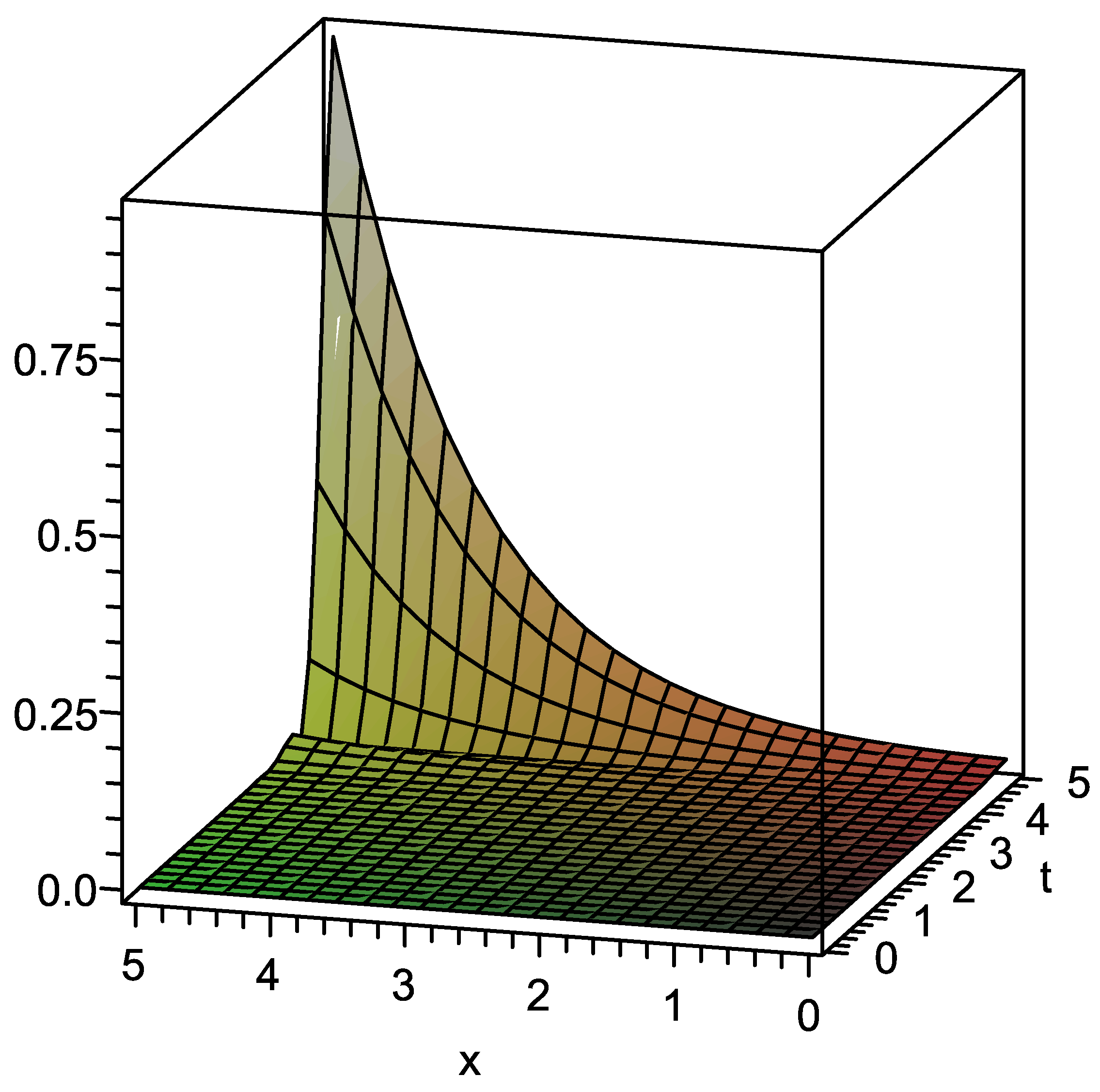
We apply a numerical integration to approximate . For obtaining an optimal value of h, we minimized by using Maple software (Waterloo Maple, Waterloo, ON, Canada). Figure 1 shows the two-dimensional variation of a seventh-order approximate solution with respect to and t for different values of . Figure 2, Figure 3 and Figure 4 describe absolute error for the 16th-order approximation by the present method for when , and . Table 1, Table 2 and Table 3 present the comparison between the absolute errors for 16th-order approximation by the present method and standard VIM for , and . The numerical results in Table 1, Table 2 and Table 3 show that the present method is effective in large domains, while the standard VIM is ineffective. Table 4 shows that in the proposed approach, the values of are close to zero compared to the standard VIM. Therefore, the present method has higher convergence speed than the exact solution to meet the standard VIM. Table 5 presents the maximum absolute error with some values of N and different values of . According to this table, increases in N decrease the arisen error of the approximation solution.
Example 2.
Consider the following fractional partial differential equation [60]:
where and the exact solution is
For obtaining an optimal value of auxiliary parameter h we define:
The value of h is obtained by minimizing where:
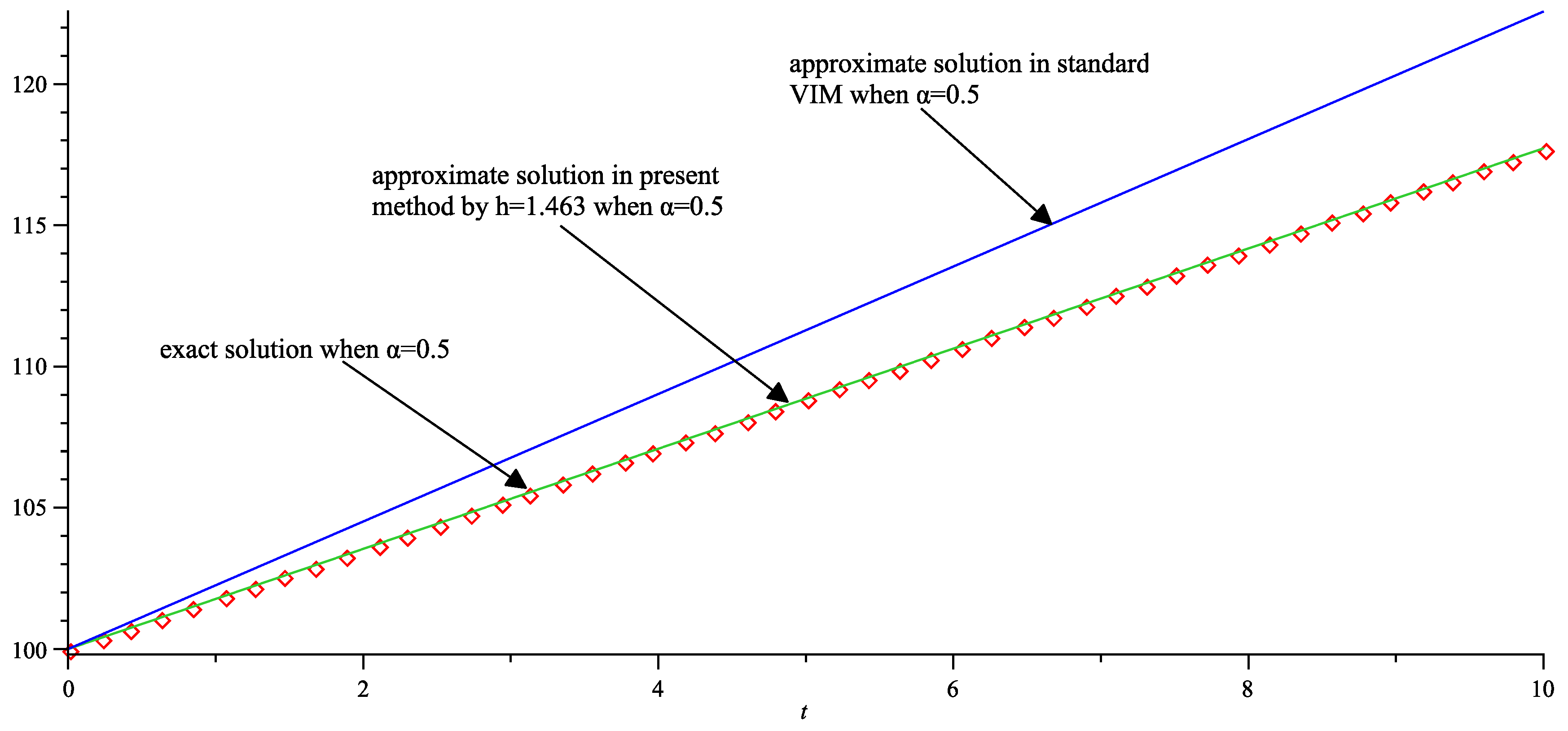
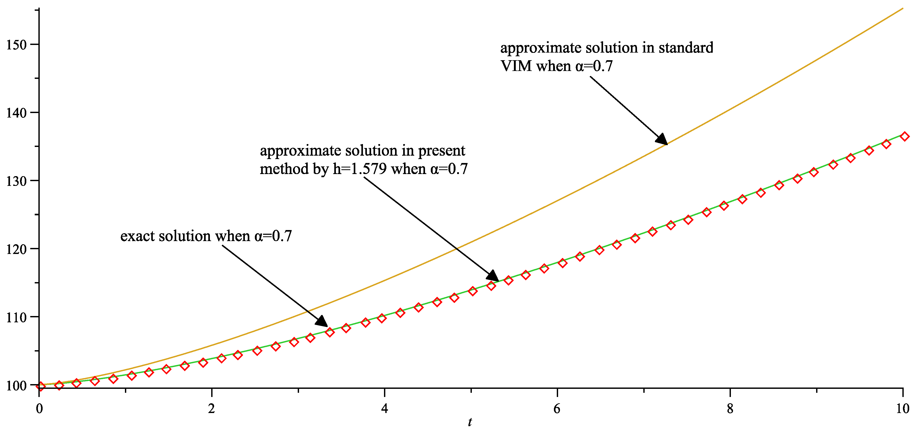
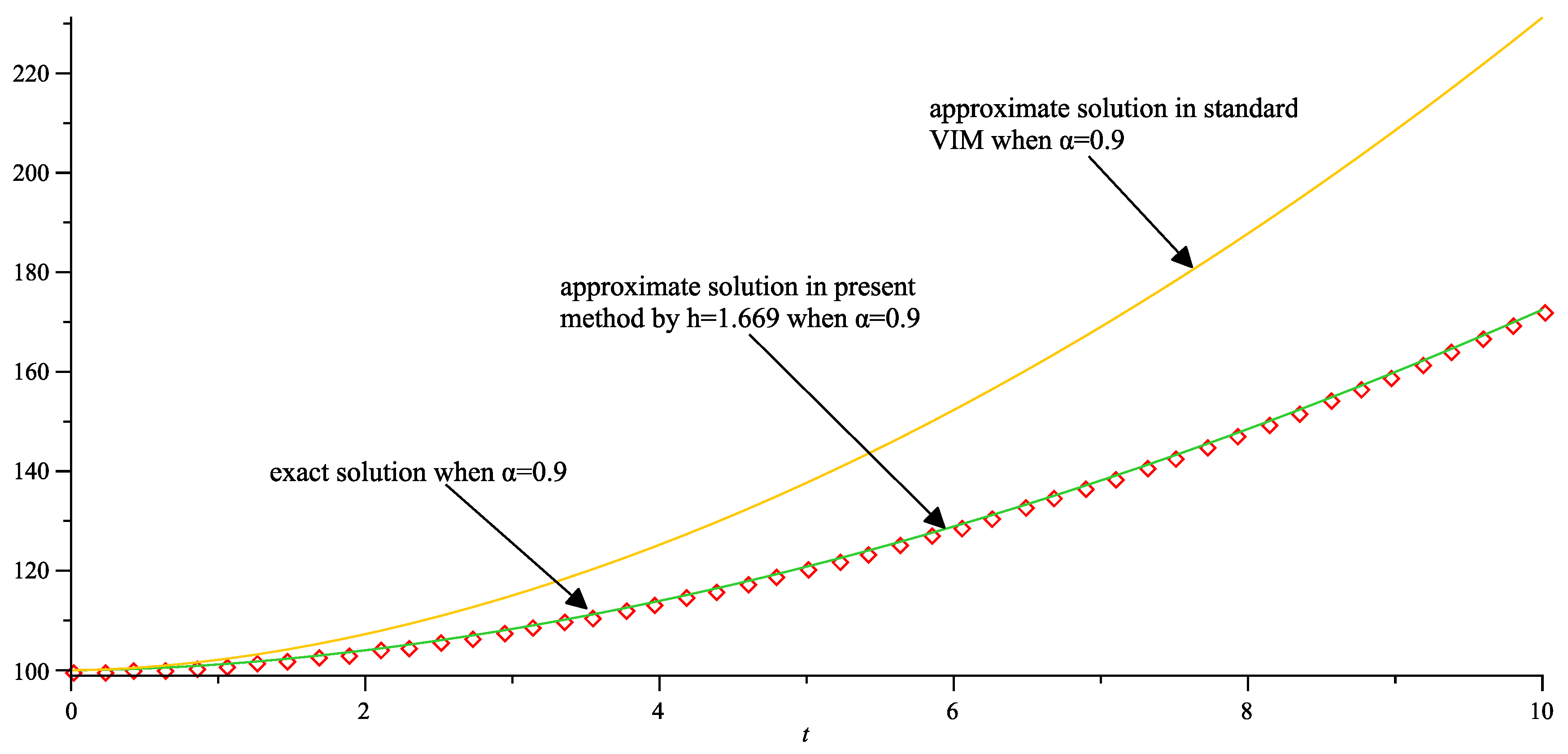
Figure 5, Figure 6 and Figure 7 show the plots of by standard VIM and VIM with an auxiliary parameter with different values of , indicating the effectiveness of the present method in large domains and ineffectiveness of standard VIM.
Example 3.
Consider the following inhomogeneous fractional convection–diffusion equation [51]:
where and the exact solution is .
We stop the solution procedure at . Here too, such as before, in order to find a suitable value of h, we define the following functions:
and:
Performing the method which is demonstrated in the above give the approximation solutions for and with :
The present method for this problem attains the exact solution for any , only by using three terms of VIM with an auxiliary parameter with
6. Conclusions
The VIM was successfully used to solve many application problems in which difficulties may arise in dealing with obtaining suitable accuracy in large domains. To overcome these difficulties, the modified VIM was proposed using VIM with an auxiliary parameter and applied to solve fractional convection–diffusion equations in this paper. Graphical figures and numerical results were presented to determine the higher accuracy and simplicity of the proposed method. In fact, our method is easy to implement, and capable of approximating solutions more accurately in longer intervals compared to the original VIM. Moreover, it should be mentioned that the propounded method can be easily generalized for more fractional problems in large domains.
Author Contributions
All of the authors provided equal contributions to the paper.
Conflicts of Interest
The authors declare no conflict of interest.
References
- Hilfer, R. (Ed.) Applications of Fractional Calculus in Physics; World Scientific: Singapore, 2000; Volume 128. [Google Scholar]
- Podlubny, I. Fractional Differential Equations: An Introduction to Fractional Derivatives, Fractional Differential Equations, to Methods of Their Solution and Some of Their Applications; Academic Press: Cambridge, MA, USA, 1998; Volume 198. [Google Scholar]
- Shawagfeh, N.T. Analytical approximate solutions for nonlinear fractional differential equations. Appl. Math. Comput. 2002, 131, 517–529. [Google Scholar] [CrossRef]
- Wazwaz, A.M. Blow-up for solutions of some linear wave equations with mixed nonlinear boundary conditions. Appl. Math. Comput. 2001, 123, 133–140. [Google Scholar] [CrossRef]
- Jafari, H.; Seifi, S. Homotopy analysis method for solving linear and nonlinear fractional diffusion-wave equation. Commun. Nonlinear Sci. Numer. Simul. 2009, 14, 2006–2012. [Google Scholar] [CrossRef]
- Wu, F.; Yang, X.J. Approximate solution of the non–linear diffusion equation of multiple orders. Therm. Sci. 2016, 20, 683–687. [Google Scholar] [CrossRef]
- Yan, S.P.; Zhong, W.P.; Yang, X.J. A novel series method for fractional diffusion equation within Caputo fractional derivative. Therm. Sci. 2016, 20, 695–699. [Google Scholar] [CrossRef]
- Gao, F.; Yang, X.J. Fractional Maxwell fluid with fractional derivative without singular kernel. Therm. Sci. 2016, 20, 871–877. [Google Scholar] [CrossRef]
- Oldham, K.; Spanier, J. The Fractional Calculus Theory and Applications of Differentiation and Integration to Arbitrary Order; Elsevier: Amsterdam, The Netherlands, 1974; Volume 111. [Google Scholar]
- Miller, K.S.; Ross, B. An Introduction to the Fractional Calculus and Fractional Differential Equations; Wiley: Hoboken, NJ, USA, 1993. [Google Scholar]
- Rossikhin, Y.A.; Shitikova, M.V. Applications of fractional calculus to dynamic problems of linear and nonlinear hereditary mechanics of solids. Appl. Mech. Rev. 1997, 50, 15–67. [Google Scholar] [CrossRef]
- Carpinteri, A.; Mainardi, F. (Eds.) Fractals and Fractional Calculus in Continuum Mechanics; Springer: Berlin, Germany, 2014; Volume 378. [Google Scholar]
- Zhang, S.; Zhang, H.Q. Fractional sub-equation method and its applications to nonlinear fractional PDEs. Phys. Lett. A 2011, 375, 1069–1073. [Google Scholar] [CrossRef]
- Caputo, M. Linear models of dissipation whose Q is almost frequency independent-II. Geophys. J. Int. 1967, 13, 529–539. [Google Scholar] [CrossRef]
- Huang, F.H.; Guo, B.L. General solutions to a class of time fractional partial differential equations. Appl. Math. Mech. 2010, 31, 815–826. [Google Scholar] [CrossRef]
- Liu, X.J.; Wang, J.Z.; Wang, X.M.; Zhou, Y.H. Exact solutions of multi-term fractional diffusion-wave equations with Robin type boundary conditions. Appl. Math. Mech. 2014, 35, 49–62. [Google Scholar] [CrossRef]
- Momani, S.; Shawagfeh, N. Decomposition method for solving fractional Riccati differential equations. Appl. Math. Comput. 2006, 182, 1083–1092. [Google Scholar] [CrossRef]
- Daftardar-Gejji, V.; Jafari, H. Solving a multi-order fractional differential equation using Adomian decomposition. Appl. Math. Comput. 2007, 189, 541–548. [Google Scholar] [CrossRef]
- Wang, Q. Numerical solutions for fractional KdV-Burgers equation by Adomian decomposition method. Appl. Math. Comput. 2006, 182, 1048–1055. [Google Scholar] [CrossRef]
- Hashim, I.; Abdulaziz, O.; Momani, S. Homotopy analysis method for fractional IVPs. Commun. Nonlinear Sci. Numer. Simul. 2009, 14, 674–684. [Google Scholar] [CrossRef]
- Zurigat, M.; Momani, S.; Alawneh, A. Analytical approximate solutions of systems of fractional algebraic-differential equations by homotopy analysis method. Comput. Math. Appl. 2010, 59, 1227–1235. [Google Scholar] [CrossRef]
- Ye, C.; Luo, X.N.; Wen, L.P. High-order numerical methods of fractional-order Stokes’ first problem for heated generalized second grade fluid. Appl. Math. Mech. 2012, 33, 65–80. [Google Scholar] [CrossRef]
- Saadatmandi, A.; Dehghan, M. A new operational matrix for solving fractional-order differential equations. Comput. Math. Appl. 2010, 59, 1326–1336. [Google Scholar] [CrossRef]
- Kumar, P.; Agrawal, O.P. An approximate method for numerical solution of fractional differential equations. Signal Process. 2006, 86, 2602–2610. [Google Scholar] [CrossRef]
- Yuste, S.B. Weighted average finite difference methods for fractional diffusion equations. J. Comput. Phys. 2006, 216, 264–274. [Google Scholar] [CrossRef]
- Wei, L.; Zhang, X.; He, Y. Analysis of a local discontinuous Galerkin method for time-fractional advection-diffusion equations. Int. J. Numer. Methods Heat Fluid Flow 2013, 23, 634–648. [Google Scholar] [CrossRef]
- Doha, E.H.; Bhrawy, A.H.; Ezz-Eldien, S.S. Efficient Chebyshev spectral methods for solving multi-term fractional orders differential equations. Appl. Math. Model. 2011, 35, 5662–5672. [Google Scholar] [CrossRef]
- Kazem, S. An integral operational matrix based on Jacobi polynomials for solving fractional-order differential equations. Appl. Math. Model. 2013, 37, 1126–1136. [Google Scholar] [CrossRef]
- Kazem, S.; Abbasbandy, S.; Kumar, S. Fractional-order Legendre functions for solving fractional-order differential equations. Appl. Math. Model. 2013, 37, 5498–5510. [Google Scholar] [CrossRef]
- Rad, J.A.; Kazem, S.; Shaban, M.; Parand, K.; Yildirim, A. Numerical solution of fractional differential equations with a Tau method based on Legendre and Bernstein polynomials. Math. Methods Appl. Sci. 2014, 37, 329–342. [Google Scholar] [CrossRef]
- He, J.H. Variational iteration method-a kind of non-linear analytical technique: some examples. Int. J. Non-Linear Mech. 1999, 34, 699–708. [Google Scholar] [CrossRef]
- Liu, H.; Xiao, A.; Su, L. Convergence of variational iteration method for second-order delay differential equations. J. Appl. Math. 2013, 2013, 634670. [Google Scholar] [CrossRef]
- Abbasbandy, S. A new application of He’s variational iteration method for quadratic Riccati differential equation by using Adomian’s polynomials. J. Comput. Appl. Math. 2007, 207, 59–63. [Google Scholar] [CrossRef]
- Salkuyeh, D.K.; Tavakoli, A. Interpolated variational iteration method for initial value problems. Appl. Math. Model. 2016, 40, 3979–3990. [Google Scholar] [CrossRef]
- Sweilam, N.H.; Khader, M.M. On the convergence of variational iteration method for nonlinear coupled system of partial differential equations. Int. J. Comput. Math. 2010, 87, 1120–1130. [Google Scholar] [CrossRef]
- Rezazadeh, G.; Madinei, H.; Shabani, R. Study of parametric oscillation of an electrostatically actuated microbeam using variational iteration method. Appl. Math. Model. 2012, 36, 430–443. [Google Scholar] [CrossRef]
- Abassy, T.A.; El-Tawil, M.A.; El Zoheiry, H. Solving nonlinear partial differential equations using the modified variational iteration Padé technique. J. Comput. Appl. Math. 2007, 207, 73–91. [Google Scholar] [CrossRef]
- Geng, F.; Lin, Y.; Cui, M. A piecewise variational iteration method for Riccati differential equations. Comput. Math. Appl. 2009, 58, 2518–2522. [Google Scholar] [CrossRef]
- Ghorbani, A.; Saberi-Nadjafi, J. An effective modification of He’s variational iteration method. Nonlinear Anal. Real World Appl. 2009, 10, 2828–2833. [Google Scholar] [CrossRef]
- Odibat, Z.; Momani, S. The variational iteration method: an efficient scheme for handling fractional partial differential equations in fluid mechanics. Comput. Math. Appl. 2009, 58, 2199–2208. [Google Scholar] [CrossRef]
- Wu, G.C. Laplace transform overcoming principle drawbacks in application of the variational iteration method to fractional heat equations. Therm. Sci. 2012, 16, 1257–1261. [Google Scholar] [CrossRef]
- Hristov, J. An exercise with the He’s variation iteration method to a fractional Bernoulli equation arising in a transient conduction with a non-linear boundary heat flux. Int. Rev. Chem. Eng. 2012, 4, 489–497. [Google Scholar]
- El-Wakil, S.A.; Abdou, M.A. New applications of variational iteration method using Adomian polynomials. Nonlinear Dyn. 2008, 52, 41–49. [Google Scholar] [CrossRef]
- Yilmaz, E.; Inc, M. Numerical simulation of the squeezing flow between two infinite plates by means of the modified variational iteration method with an auxiliary parameter. Nonlinear Sci. Lett. A 2010, 1, 297–306. [Google Scholar]
- Hosseini, M.M.; Mohyud-Din, S.T.; Ghaneai, H.; Usman, M. Auxiliary parameter in the variational iteration method and its optimal determination. Int. J. Nonlinear Sci. Numer. Simul. 2010, 11, 495–502. [Google Scholar] [CrossRef]
- Turkyilmazoglu, M. An optimal variational iteration method. Applied Mathematics Letters 2011, 24, 762–765. [Google Scholar] [CrossRef]
- Herisanu, N.; Marinca, V. A modified variational iteration method for strongly nonlinear problems. Nonlinear Sci. Lett. A 2010, 1, 183–192. [Google Scholar]
- Turkyilmazoglu, M. Convergent optimal variational iteration method and applications to heat and fluid flow problems. Int. J. Numer. Methods Heat Fluid Flow 2016, 26, 790–804. [Google Scholar] [CrossRef]
- Momani, S. An algorithm for solving the fractional convection-diffusion equation with nonlinear source term. Commun. Nonlinear Sci. Numer. Simul. 2007, 12, 1283–1290. [Google Scholar] [CrossRef]
- Merdan, M. Analytical approximate solutions of fractional convection-diffusion equation with modified Riemann-Liouville derivative by means of fractional variational iteration method. Iran. J. Sci. Technol. Sci. 2013, 37, 83–92. [Google Scholar]
- Abbasbandy, S.; Kazem, S.; Alhuthali, M.S.; Alsulami, H.H. Application of the operational matrix of fractional-order Legendre functions for solving the time-fractional convection-diffusion equation. Appl. Math. Comput. 2015, 266, 31–40. [Google Scholar] [CrossRef]
- Gorenflo, R.; Mainardi, F. Fractional Calculus; Springer: Vienna, Austria, 1997; pp. 223–276. [Google Scholar]
- Liu, Y. Studies on boundary value problems of singular fractional differential equations with impulse effects. Rostock. Math. Kolloqu. 2015, 70, 3–108. [Google Scholar]
- Wang, K.; Liu, S. A new solution procedure for nonlinear fractional porous media equation based on a new fractional derivative. Nonlinear Sci. Lett. A Math. Phys. Mech. 2017, 135. [Google Scholar]
- Wang, K.L.; Liu, S.Y. He’s fractional derivative for non-linear fractional heat transfer equation. Therm. Sci. 2016, 20, 793–796. [Google Scholar] [CrossRef]
- Odibat, Z.M. A study on the convergence of variational iteration method. Math. Comput. Model. 2010, 51, 1181–1192. [Google Scholar] [CrossRef]
- Ghaneai, H.; Hosseini, M.M. Variational iteration method with an auxiliary parameter for solving wave-like and heat-like equations in large domains. Comput. Math. Appl. 2015, 69, 363–373. [Google Scholar] [CrossRef]
- Ghaneai, H.; Hosseini, M.M. Solving differential-algebraic equations through variational iteration method with an auxiliary parameter. Appl. Math. Model. 2015, 40, 3991–4001. [Google Scholar] [CrossRef]
- Ghaneai, H.; Hosseini, M.M.; Tauseef Mohyud-Din, S. Modified variational iteration method for solving a neutral functional-differential equation with proportional delays. Int. J. Numer. Methods Heat Fluid Flow 2012, 22, 1086–1095. [Google Scholar] [CrossRef]
- Chen, Y.; Wu, Y.; Cui, Y.; Wang, Z.; Jin, D. Wavelet method for a class of fractional convection-diffusion equation with variable coefficients. J. Comput. Sci. 2010, 1, 146–149. [Google Scholar] [CrossRef]
Figure 1.
Plots of seventh-order approximation solutions by present method at for different values of in Example 1.
Figure 1.
Plots of seventh-order approximation solutions by present method at for different values of in Example 1.
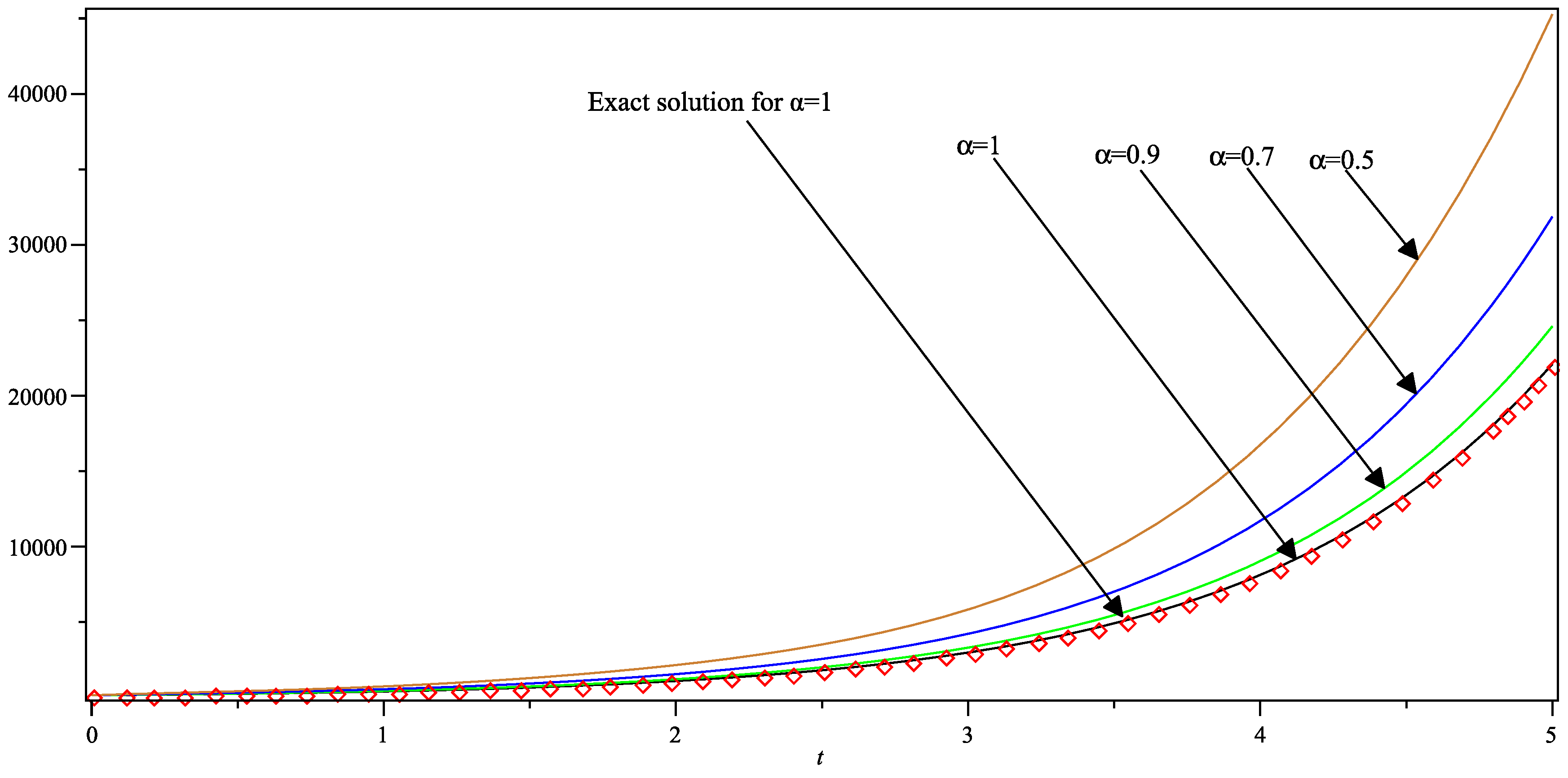
Figure 2.
Absolute error for the 16th-order approximation by present method for when and in Example 1.
Figure 2.
Absolute error for the 16th-order approximation by present method for when and in Example 1.

Figure 3.
Absolute error for the 16th-order approximation by present method for when and in Example 1.
Figure 3.
Absolute error for the 16th-order approximation by present method for when and in Example 1.
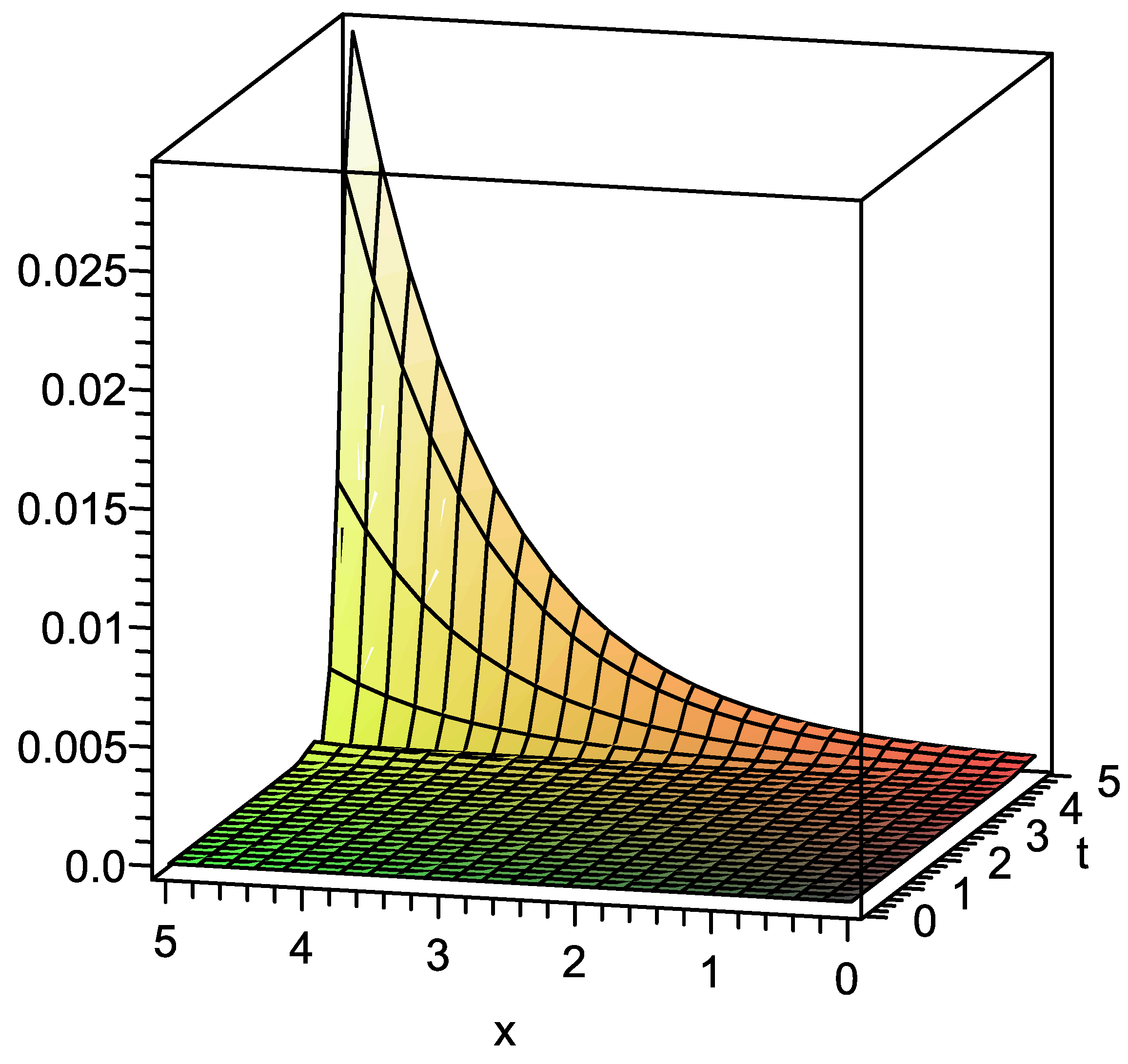
Figure 4.
Absolute error for the 16th-order approximation by present method for when and in Example 1.
Figure 4.
Absolute error for the 16th-order approximation by present method for when and in Example 1.
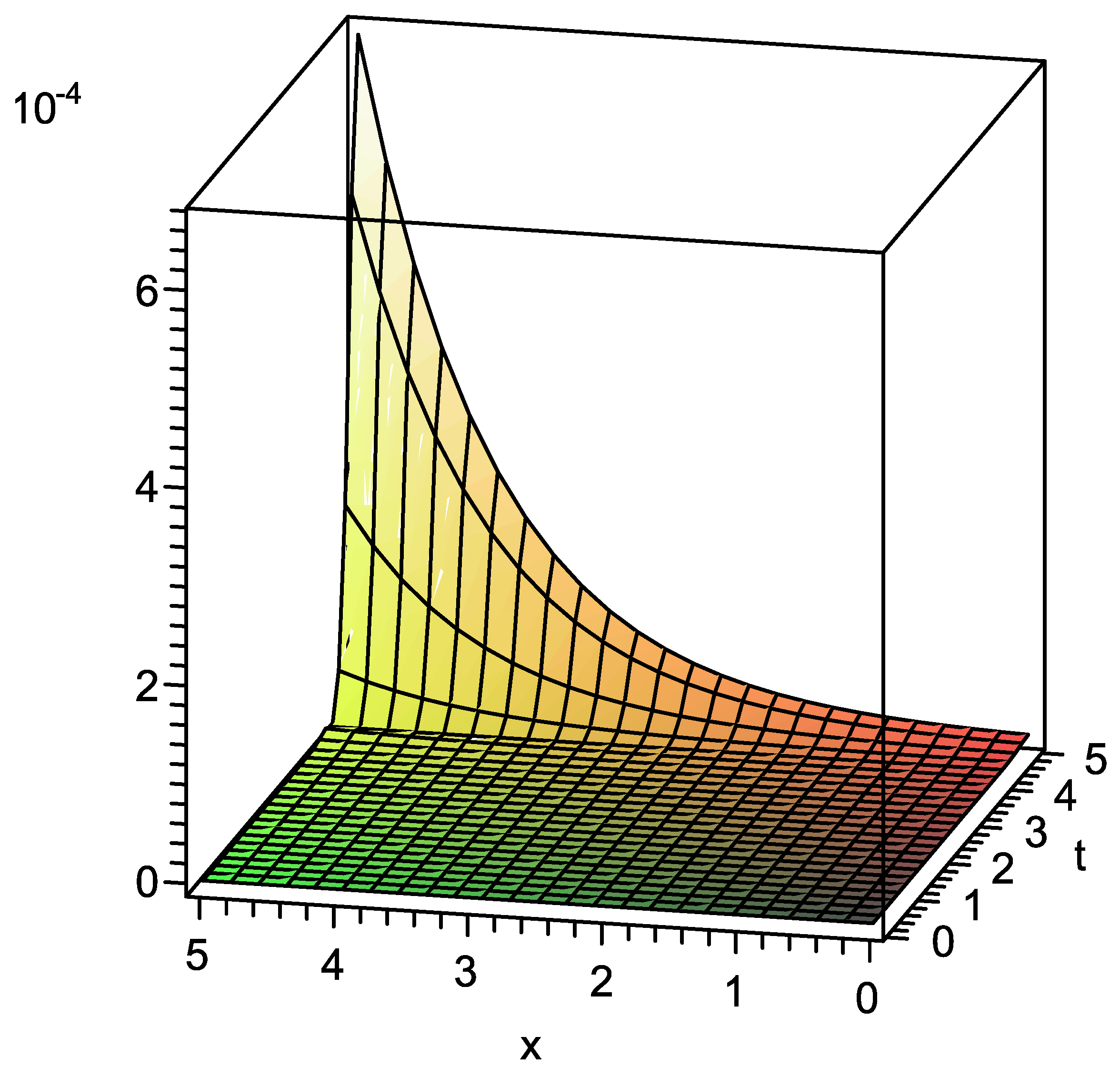
Figure 5.
Plots of third-order approximation solutions by present method and standard VIM at for in Example 2.
Figure 5.
Plots of third-order approximation solutions by present method and standard VIM at for in Example 2.

Figure 6.
Plots of third-order approximation solutions by present method and standard VIM at for in Example 2.
Figure 6.
Plots of third-order approximation solutions by present method and standard VIM at for in Example 2.

Figure 7.
Plots of third-order approximation solutions by present method and standard VIM at for in Example 2.
Figure 7.
Plots of third-order approximation solutions by present method and standard VIM at for in Example 2.


Table 1.
Comparison of absolute errors for 16th-order approximation by present method with and standard variational iteration method (VIM), when in Example 1.
Table 1.
Comparison of absolute errors for 16th-order approximation by present method with and standard variational iteration method (VIM), when in Example 1.
| x | t | Absolute Error in Present Method | Absolute Error in Standard VIM |
|---|---|---|---|
| 0.5 | 0.5 | ||
| 1 | 1 | ||
| 1.5 | 1.5 | ||
| 2 | 2 | ||
| 2.5 | 2.5 | ||
| 3 | 3 | ||
| 3.5 | 3.5 | ||
| 4 | 4 | ||
| 4.5 | 4.5 | ||
| 5 | 5 |
Table 2.
Comparison of absolute errors for 16th-order approximation by present method with and standard VIM, when in Example 1.
Table 2.
Comparison of absolute errors for 16th-order approximation by present method with and standard VIM, when in Example 1.
| x | t | Absolute Error in Present Method | Absolute Error in Standard VIM |
|---|---|---|---|
| 0.5 | 0.5 | ||
| 1 | 1 | ||
| 1.5 | 1.5 | ||
| 2 | 2 | ||
| 2.5 | 2.5 | ||
| 3 | 3 | ||
| 3.5 | 3.5 | ||
| 4 | 4 | ||
| 4.5 | 4.5 | ||
| 5 | 5 |
Table 3.
Comparison of absolute errors for 16th-order approximation by present method with and standard VIM, when in Example 1.
Table 3.
Comparison of absolute errors for 16th-order approximation by present method with and standard VIM, when in Example 1.
| x | t | Absolute Error in Present Method | Absolute Error in Standard VIM |
|---|---|---|---|
| 0.5 | 0.5 | ||
| 1 | 1 | ||
| 1.5 | 1.5 | ||
| 2 | 2 | ||
| 2.5 | 2.5 | ||
| 3 | 3 | ||
| 3.5 | 3.5 | ||
| 4 | 4 | ||
| 4.5 | 4.5 | ||
| 5 | 5 |
Table 4.
Values of defended in (16) for present method and standard VIM with in Example 1.
Table 4.
Values of defended in (16) for present method and standard VIM with in Example 1.
| Present | Standard | Present | Standard | Present | Standard | Present | Standard | |
|---|---|---|---|---|---|---|---|---|
| Method | VIM | Method | VIM | Method | VIM | Method | VIM | |
Table 5.
The maximum absolute error with some N and various values of by present method for Example 1.
Table 5.
The maximum absolute error with some N and various values of by present method for Example 1.
| N | ||||
|---|---|---|---|---|
| 14 | ||||
| 16 | ||||
| 18 | ||||
| 20 |
© 2017 by the authors. Licensee MDPI, Basel, Switzerland. This article is an open access article distributed under the terms and conditions of the Creative Commons Attribution (CC BY) license (http://creativecommons.org/licenses/by/4.0/).
Share and Cite
MDPI and ACS Style
Abolhasani, M.; Abbasbandy, S.; Allahviranloo, T. A New Variational Iteration Method for a Class of Fractional Convection-Diffusion Equations in Large Domains. Mathematics 2017, 5, 26. https://doi.org/10.3390/math5020026
AMA Style
Abolhasani M, Abbasbandy S, Allahviranloo T. A New Variational Iteration Method for a Class of Fractional Convection-Diffusion Equations in Large Domains. Mathematics. 2017; 5(2):26. https://doi.org/10.3390/math5020026
Chicago/Turabian StyleAbolhasani, Mohammad, Saeid Abbasbandy, and Tofigh Allahviranloo. 2017. "A New Variational Iteration Method for a Class of Fractional Convection-Diffusion Equations in Large Domains" Mathematics 5, no. 2: 26. https://doi.org/10.3390/math5020026
Note that from the first issue of 2016, this journal uses article numbers instead of page numbers. See further details here.