Fusion Estimation from Multisensor Observations with Multiplicative Noises and Correlated Random Delays in Transmission

Abstract

In this paper, the information fusion estimation problem is investigated for a class of multisensor linear systems affected by different kinds of stochastic uncertainties, using both the distributed and the centralized fusion methodologies. It is assumed that the measured outputs are perturbed by one-step autocorrelated and cross-correlated additive noises, and also stochastic uncertainties caused by multiplicative noises and randomly missing measurements in the sensor outputs are considered. At each sampling time, every sensor output is sent to a local processor and, due to some kind of transmission failures, one-step correlated random delays may occur. Using only covariance information, without requiring the evolution model of the signal process, a local least-squares (LS) filter based on the measurements received from each sensor is designed by an innovation approach. All these local filters are then fused to generate an optimal distributed fusion filter by a matrix-weighted linear combination, using the LS optimality criterion. Moreover, a recursive algorithm for the centralized fusion filter is also proposed and the accuracy of the proposed estimators, which is measured by the estimation error covariances, is analyzed by a simulation example.

1. Introduction

Over the past decades, the use of sensor networks has experienced a fast development encouraged by the wide range of potential applications in many areas, since they usually provide more information than traditional single-sensor communication systems. So, important advances have been achieved concerning the estimation problem in networked stochastic systems and the design of multisensor fusion techniques [1]. Many of the existing fusion estimation algorithms are related to conventional systems (see e.g., [2,3,4,5], and the references therein), where the sensor measured outputs are affected only by additive noises and each sensor transmits its outputs to the fusion center over perfect connections.

However, in a network context, usually the restrictions of the physical equipment or the uncertainties in the external environment, inevitably cause problems in both the sensor outputs and the transmission of such outputs, that can worsen dramatically the quality of the fusion estimators designed without considering these drawbacks [6]. Multiplicative noise uncertainties and missing measurements are some of the random phenomena that usually arise in the sensor measured outputs and motivate the design of new estimation algorithms (see e.g., [7,8,9,10,11], and references therein).

Furthermore, when the sensors send their measurements to the processing center via a communication network some additional network-induced phenomena, such as random delays or measurement losses, inevitably arise during this transmission process, which can spoil the fusion estimators performance and motivate the design of fusion estimation algorithms for systems with one (or even several) of the aforementioned uncertainties (see e.g., [12,13,14,15,16,17,18,19,20,21,22,23,24], and references therein). All the above cited papers on signal estimation with random transmission delays assume independent random delays at each sensor and mutually independent delays between the different sensors; in [25] this restriction was weakened and random delays featuring correlation at consecutive sampling times were considered, thus allowing to deal with some common practical situations (e.g., those in which two consecutive observations cannot be delayed).

It should be also noted that, in many real-world problems, the measurement noises are usually correlated; this occurs, for example, when all the sensors operate in the same noisy environment or when the sensor noises are state-dependent. For this reason, the fairly conservative assumption that the measurement noises are uncorrelated is commonly weakened in many of the aforementioned research papers on signal estimation. Namely, the optimal Kalman filtering fusion problem in systems with noise cross-correlation at consecutive sampling times is addressed, for example, in [19]; also, under different types of noise correlation, centralized and distributed fusion algorithms for systems with multiplicative noise are obtained in [11,20], and for systems where the measurements might have partial information about the signal in [7].

In this paper, covariance information is used to address the distributed and centralized fusion estimation problems for a class of linear networked stochastic systems with multiplicative noises and missing measurements in the sensor measured outputs, subject to transmission random one-step delays. It is assumed that the sensor measurement additive noises are one-step autocorrelated and cross-correlated, and the Bernoulli variables describing the measurement delays at the different sensors are correlated at the same and consecutive sampling times. As in [25], correlated random delays in the transmission are assumed to exist, with different delay rates at each sensor; however, the proposed observation model is more general than that considered in [25] since, besides the random delays in the transmission, multiplicative noises and missing phenomena in the measured outputs are considered; also cross-correlation between the different sensor additive noises is taken into account. Unlike [7,8,9,10,11] where multiplicative noise uncertainties and/or missing measurements are considered in the sensor measured outputs, in this paper random delays in the transmission are also assumed to exist. Hence, a unified framework is provided for dealing simultaneously with missing measurements and uncertainties caused by multiplicative noises, along with random delays in the transmission and, hence, the proposed fusion estimators have wide applicability. Recursive algorithms for the optimal linear distributed and centralized filters under the least-squares (LS) criterion are derived by an innovation approach. Firstly, local estimators based on the measurements received from each sensor are obtained and then the distributed fusion filter is generated as the LS matrix-weighted linear combination of the local estimators. Also, a recursive algorithm for the optimal linear centralized filter is proposed. Finally, it is important to note that, even though the state augmentation method has been largely used in the literature to deal with the measurement delays, such method leads to a significant rise of the computational burden, due to the increase of the state dimension. In contrast to such approach, the fusion estimators proposed in the current paper are obtained without needing the state augmentation; so, the dimension of the designed estimators is the same as that of the original state, thus reducing the computational cost compared with the existing algorithms based on the augmentation method.

The rest of the paper is organized as follows. The multisensor measured output model with multiplicative noises and missing measurements, along with the transmission random one-step delay model, are presented in Section 2. The distributed fusion estimation algorithm is derived in Section 3, and a recursive algorithm for the centralized LS linear filtering estimator is proposed in Section 4. The effectiveness of the proposed estimation algorithms is analyzed in Section 5 by a simulation example and some conclusions are drawn in Section 6.

Notation: The notation throughout the paper is standard. ${\mathbb{R}}^n$ and ${\mathbb{R}}^{m\times n}$ denote the n-dimensional Euclidean space and the set of all $m\times n$ real matrices, respectively. For a matrix A, the symbols $A^T$ and $A^{-1}$ denote its transpose and inverse, respectively; the notation $A\otimes B$ represents the Kronecker product of the matrices $A,B$. If the dimensions of vectors or matrices are not explicitly stated, they are assumed to be compatible with algebraic operations. In particular, I denotes the identity matrix of appropriate dimensions. The notation $a\wedge b$ indicates the minimum value of two real numbers $a,b$. For any function $G_{k,s}$, depending on the time instants k and s, we will write $G_k=G_{k,k}$ for simplicity; analogously, $F^{\left(i\right)}=F^{\left(ii\right)}$ will be written for any function $F^{\left(ij\right)}$, depending on the sensors i and j. Moreover, for an arbitrary random vector ${\alpha }_k^{\left(i\right)}$, we will use the notation ${\overline{\alpha }}_k^{\left(i\right)}\equiv E\left[{\alpha }_k^{\left(i\right)}\right]$, where $E[.]$ is the mathematical expectation operator. Finally, ${\delta }_{k,s}$ denotes the Kronecker delta function.

2. Problem Formulation and Model Description

This paper is concerned with the LS linear filtering estimation problem of discrete-time stochastic signals from randomly delayed observations coming from networked sensors using the distributed and centralized fusion methods. The signal measurements at the different sensors are affected by multiplicative and additive noises, and the additive sensor noises are assumed to be correlated and cross-correlated at the same and consecutive sampling times. Each sensor output is transmitted to a local processor over imperfect network connections and, due to network congestion or some other causes, random one-step delays may occur during this transmission process; in order to model different delay rates in the transmission from each sensor to the local processor, different sequences of correlated Bernoulli random variables with known probability distributions are used.

In the distributed fusion method, each local processor produces the LS linear filter based on the measurements received from the sensor itself; afterwards, these local estimators are transmitted to the fusion center over perfect connections, and the distributed fusion filter is generated by a matrix-weighted linear combination of the local LS linear filtering estimators using the mean squared error as optimality criterion. In the centralized fusion method, all measurement data of the local processors are transmitted to the fusion center, also over perfect connections, and the LS linear filter based on all the measurements received is obtained by a recursive algorithm.

Next, we present the observation model and the hypotheses on the signal and noise processes necessary to address the estimation problem.

2.1. Signal Process

The distributed and centralized fusion filtering estimators will be obtained under the assumption that the evolution model of the signal to be estimated is unknown and only information about its mean and covariance functions is available; specifically, the following hypothesis is required:

Hypothesis 1.

The $n_x$-dimensional signal process ${\left\{x_k\right\}}_{k\ge 1}$ has zero mean and its autocovariance function is expressed in a separable form, $E\left[x_k{x}_s^T\right]=A_k{B}_s^T,s\le k,$ where $A_k,B_s\in {\mathbb{R}}^{n_x\times n}$ are known matrices.

Note that, when the system matrix $\mathsf{\Phi }$ in the state-space model of a stationary signal is available, the signal autocovariance function is $E\left[x_k{x}_s^T\right]={\mathsf{\Phi }}^{k-s}E\left[x_s{x}_s^T\right],s\le k,$ and Hypothesis 1 is clearly satisfied taking, for example, $A_k={\mathsf{\Phi }}^k$ and $B_s=E\left[x_s{x}_s^T\right]{\left({\mathsf{\Phi }}^{-s}\right)}^T$. Similarly, if $x_k={\mathsf{\Phi }}_{k-1}{x}_{k-1}+w_{k-1}$, the covariance function can be expressed as $E\left[x_k{x}_s^T\right]={\mathsf{\Phi }}_{k,s}E\left[x_s{x}_s^T\right],s\le k,$ where ${\mathsf{\Phi }}_{k,s}={\mathsf{\Phi }}_{k-1}\cdots {\mathsf{\Phi }}_s$, and Hypothesis 1 is also satisfied taking $A_k={\mathsf{\Phi }}_{k,0}$ and $B_s=E\left[x_s{x}_s^T\right]{({\mathsf{\Phi }}_{s,0}^{-1})}^T$. Furthermore, Hypothesis 1 covers even situations where the system matrix in the state-space model is singular, although a different factorization must be used in those cases (see e.g., [21]). Hence, Hypothesis 1 on the signal autocovariance function covers both stationary and non-stationary signals, providing a unified context to deal with a large number of different situations and avoiding the derivation of specific algorithms for each of them.

2.2. Multisensor Measured Outputs

Consider m sensors, whose measurements obey the following equations:

$$z_k^{\left(i\right)}={\theta }_k^{\left(i\right)}\left(H_k^{\left(i\right)}+{\epsilon }_k^{\left(i\right)}{C}_k^{\left(i\right)}\right)x_k+v_k^{\left(i\right)},k\ge 1,i=1,\dots ,m$$

(1)

where $z_k^{\left(i\right)}\in {\mathbb{R}}^{n_z}$ is the measured output of the i-th sensor at time k, which is transmitted to a local processor by unreliable network connections, and $H_k^{\left(i\right)}$, $C_k^{\left(i\right)}$ are known time-varying matrices of suitable dimensions. For each sensor $i=1,\dots ,m,$${\{{\theta }_k^{\left(i\right)}\}}_{k\ge 1}$ is a Bernoulli process describing the missing phenomenon, ${\{{\epsilon }_k^{\left(i\right)}\}}_{k\ge 1}$ is a scalar multiplicative noise, and ${\{v_k^{\left(i\right)}\}}_{k\ge 1}$ is the measurement noise.

The following hypotheses on the observation model given by Equation (1) are required:

Hypothesis 2.

The processes ${\{{\theta }_k^{\left(i\right)}\}}_{k\ge 1}$, $i=1,\dots ,m$, are independent sequences of independent Bernoulli random variables with know probabilities $P({\theta }_k^{\left(i\right)}=1)={\overline{\theta }}_k^{\left(i\right)},k\ge 1$.

Hypothesis 3.

The multiplicative noises ${\{{\epsilon }_k^{\left(i\right)}\}}_{k\ge 1}$, $i=1,\dots ,m$, are independent sequences of independent scalar random variables with zero means and known second-order moments; we will denote ${\sigma }_k^{\left(i\right)}\equiv E\left[{({\epsilon }_k^{\left(i\right)})}^2\right],k\ge 1$.

Hypothesis 4.

The sensor measurement noises ${\{v_k^{\left(i\right)}\}}_{k\ge 1},i=1,\dots ,m$, are zero-mean sequences with known second-order moments defined by:

$$E[v_k^{\left(i\right)}{v}_s^{\left(j\right)T}]=R_k^{\left(ij\right)}{\delta }_{k,s}+R_{k,k-1}^{\left(ij\right)}{\delta }_{k-1,s},s\le k;i,j=1,\dots ,m$$

From Hypothesis 2, different sequences of independent Bernoulli random variables with known probabilities are used to model the phenomenon of missing measurements at each sensor; so, when ${\theta }_k^{\left(i\right)}=1$, which occurs with known probability ${\overline{\theta }}_k^{\left(i\right)}$, the state $x_k$ is present in the measurement $z_k^{\left(i\right)}$ coming from the i-th sensor at time k; otherwise, ${\theta }_k^{\left(i\right)}=0$ and the state is missing in the measured output from the i-th sensor at time k, which means that such observation only contains additive noise $v_k^{\left(i\right)}$ with probability $1-{\overline{\theta }}_k^{\left(i\right)}$. Although these variables are assumed to be independent from sensor to sensor, such condition is not necessary to deduce either the centralized estimators or the local estimators, but only to obtain the cross-covariance matrices of the local estimation errors, which are necessary to determine the matrix weights of the distributed fusion estimators. Concerning Hypothesis 3, it should be noted that the multiplicative noises involved in uncertain systems are usually gaussian noises. Finally, note that the conservative hypothesis of independence between different sensor measurement noises has been weakened in Hypothesis 4, since such independence assumption may be a limitation in many real-world problems; for example, when all the sensors operate in the same noisy environment, the noises are usually correlated, or even some sensors may have the same measurement noises.

2.3. Observation Model with Random One-Step Delays

For each $k\ge 1$, assume that the measured outputs of the different sensors, $z_k^{\left(i\right)}$, $i=1,\dots ,m$, are transmitted to the local processors through unreliable communication channels and, due to network congestion or some other causes, random one-step delays with different rates are supposed to exist in these transmissions. Assuming that the first measurement is always available and considering different sequences of Bernoulli random variables, ${\{{\gamma }_k^{\left(i\right)}\}}_{k\ge 2}$, $i=1,\dots ,m$, to model the random delays, the observations used in the estimation are described by:

$$y_k^{\left(i\right)}=(1-{\gamma }_k^{\left(i\right)})z_k^{\left(i\right)}+{\gamma }_k^{\left(i\right)}{z}_{k-1}^{\left(i\right)},k\ge 2;y_1^{\left(i\right)}=z_1^{\left(i\right)};i=1,\dots ,m$$

(2)

From Equation (2) it is clear that ${\gamma }_k^{\left(i\right)}=0$ means that $y_k^{\left(i\right)}=z_k^{\left(i\right)}$; that is, the local processor receives the data from the i-th sensor at the sampling time k. When ${\gamma }_k^{\left(i\right)}=1$, then $y_k^{\left(i\right)}=z_{k-1}^{\left(i\right)}$, meaning that the measured output at time k is delayed and the previous one $z_{k-1}^{\left(i\right)}$ is used for the estimation. These Bernoulli random variables modelling the delays are assumed to be one-step correlated, thus covering many practical situations; for example, those in which consecutive observations transmitted through the same channel cannot be delayed, or situations where there are some sort of links between the different communications channels. Specifically, the following hypothesis is assumed:

Hypothesis 5.

${\{{\gamma }_k^{\left(i\right)}\}}_{k\ge 2}$, $i=1,\dots ,m,$ are sequences of Bernoulli random variables with known means, ${\overline{\gamma }}_k^{\left(i\right)}\equiv E[{\gamma }_k^{\left(i\right)}],k\ge 2$. It is assumed that ${\gamma }_k^{\left(i\right)}$ and ${\gamma }_s^{\left(j\right)}$ are independent for $|k-s|\ge 2$, and the second-order moments, ${\overline{\gamma }}_{k,s}^{(i,j)}\equiv E[{\gamma }_k^{\left(i\right)}{\gamma }_s^{\left(j\right)}],s=k-1,k,$ and $i,j=1,\dots ,m,$ are also known.

Finally, the following independence hypothesis is also required:

Hypothesis 6.

For $i=1,\dots ,m$, the processes ${\left\{x_k\right\}}_{k\ge 1}$, ${\{{\theta }_k^{\left(i\right)}\}}_{k\ge 1}$, ${\{{\epsilon }_k^{\left(i\right)}\}}_{k\ge 1}$, ${\{v_k^{\left(i\right)}\}}_{k\ge 1}$ and ${\{{\gamma }_k^{\left(i\right)}\}}_{k\ge 2}$ are mutually independent.

In the following proposition, explicit expressions for the autocovariance functions of the transmitted and received measurements, that will be necessary for the distributed fusion estimation algorithm, are derived.

Proposition 1.

For $i,j=1,\dots ,m$, the autocovariance functions ${\mathsf{\Sigma }}_{k,s}^{z^{\left(ij\right)}}\equiv E[z_k^{\left(i\right)}{z}_s^{\left(j\right)T}]$ and ${\mathsf{\Sigma }}_{k,s}^{y^{\left(i\right)}}\equiv E[y_k^{\left(i\right)}{y}_s^{\left(i\right)T}]$ are given by:

$$\begin{array}{c}{\mathsf{\Sigma }}_k^{z^{\left(i\right)}}={\overline{\theta }}_k^{\left(i\right)}{H}_k^{\left(i\right)}{A}_k{B}_k^T{H}_k^{\left(i\right)T}+{\sigma }_k^{\left(i\right)}{C}_k^{\left(i\right)}{A}_k{B}_k^T{C}_k^{\left(i\right)T}+R_k^{\left(i\right)},k\ge 1\hfill \\ {\mathsf{\Sigma }}_{k,s}^{z^{\left(ij\right)}}={\overline{\theta }}_k^{\left(i\right)}{\overline{\theta }}_s^{\left(j\right)}{H}_k^{\left(i\right)}{A}_k{B}_s^T{H}_s^{\left(j\right)T}+R_{k,k-1}^{\left(ij\right)}{\delta }_{k-1,s}+R_k^{\left(ij\right)}{\delta }_{k,s},i\ne j,ors<k\hfill \\ {\mathsf{\Sigma }}_{k,s}^{y^{\left(ij\right)}}=(1-{\overline{\gamma }}_k^{\left(i\right)}-{\overline{\gamma }}_s^{\left(j\right)}+{\overline{\gamma }}_{k,s}^{(i,j)}){\mathsf{\Sigma }}_{k,s}^{z^{\left(ij\right)}}+({\overline{\gamma }}_s^{\left(j\right)}-{\overline{\gamma }}_{k,s}^{(i,j)}){\mathsf{\Sigma }}_{k,s-1}^{z^{\left(ij\right)}}\hfill \\ \phantom{{\mathsf{\Sigma }}_{k,s}^{y^{\left(ij\right)}}=}+({\overline{\gamma }}_k^{\left(i\right)}-{\overline{\gamma }}_{k,s}^{(i,j)}){\mathsf{\Sigma }}_{k-1,s}^{z^{\left(ij\right)}}+{\overline{\gamma }}_{k,s}^{(i,j)}{\mathsf{\Sigma }}_{k-1,s-1}^{z^{\left(ij\right)}},k,s\ge 2\hfill \\ {\mathsf{\Sigma }}_{2,1}^{y^{\left(ij\right)}}=(1-{\overline{\gamma }}_2^{\left(i\right)}){\mathsf{\Sigma }}_{2,1}^{z^{\left(ij\right)}}+{\overline{\gamma }}_2^{\left(i\right)}{\mathsf{\Sigma }}_1^{z^{\left(ij\right)}};{\mathsf{\Sigma }}_1^{y^{\left(ij\right)}}={\mathsf{\Sigma }}_1^{z^{\left(ij\right)}}\hfill \end{array}$$

(3)

Proof. 

From Equations (1) and (2), taking into account Hypotheses 1–6, the expressions given in Equation (3) are easily obtained. ☐

3. Distributed Fusion Linear Filter

In this section, we address the distributed fusion linear filtering problem of the signal from the randomly delayed observations defined by Equations (1) and (2), using the LS optimality criterion. In the distributed fusion method, each local processor provides the LS linear filter of the signal $x_k$ based on the measurements from the corresponding sensor, which will be denoted by ${\widehat{x}}_{k/k}^{\left(i\right)}$; afterwards, these local filters are transmitted to the fusion center where the distributed filter, ${\widehat{x}}_{k/k}^{\left(D\right)}$, is designed as a matrix-weighted linear combination of such local filters. First, in Section 3.1, for each $i=1,\dots ,m$, a recursive algorithm for the local LS linear filter, ${\widehat{x}}_{k/k}^{\left(i\right)}$, will be deduced. Then, in Section 3.2, the derivation of the cross-correlation matrices between any two local filters, ${\widehat{\mathsf{\Sigma }}}_{k/k}^{\left(ij\right)}=E[{\widehat{x}}_{k/k}^{\left(i\right)}{\widehat{x}}_{k/k}^{\left(j\right)T}]$, $i,j=1,\dots ,m$, will be detailed. Finally, in Section 3.3, the distributed fusion filter weighted by matrices, ${\widehat{x}}_{k/k}^{\left(D\right)}$, will be generated from the local filters by applying the LS optimality criterion.

3.1. Local LS Linear Filtering Recursive Algorithm

To obtain the signal LS linear filters based on the available observations from each sensor, we will use an innovation approach. For each sensor $i=1,\dots ,m$, the innovation at time k, which represents the new information provided by the k-th observation, is defined by ${\mu }_k^{\left(i\right)}=y_k^{\left(i\right)}-{\widehat{y}}_{k/k-1}^{\left(i\right)},k\ge 1$, where ${\widehat{y}}_{k/k-1}^{\left(i\right)}$ is the LS linear estimator of $y_k$ based on the previous observations, $y_s^{\left(i\right)},s\le k-1$, with ${\widehat{y}}_{1/0}^{\left(i\right)}=E[y_1^{\left(i\right)}]=0$.

As it is known (see e.g., [26]), the innovations, ${\{{\mu }_k^{\left(i\right)}\}}_{k\ge 1}$, constitute a zero-mean white process, and the LS linear estimator of any random vector ${\alpha }_k$ based on the observations $y_1^{\left(i\right)},\dots ,y_L^{\left(i\right)}$, denoted by ${\widehat{\alpha }}_{k/L}^{\left(i\right)}$, can be calculated as a linear combination of the corresponding innovations, ${\mu }_1^{\left(i\right)},\dots ,{\mu }_L^{\left(i\right)}$; namely

$${\widehat{\alpha }}_{k/L}^{\left(i\right)}=\sum _{h=1}^{L}E[{\alpha }_k{\mu }_h^{\left(i\right)T}]{\mathsf{\Pi }}_h^{\left(i\right)-1}{\mu }_h^{\left(i\right)}$$

(4)

where ${\mathsf{\Pi }}_h^{\left(i\right)}\equiv E[{\mu }_h^{\left(i\right)}{\mu }_h^{\left(i\right)T}]$ denotes the covariance matrix of ${\mu }_h^{\left(i\right)}$.

This general expression for the LS linear estimators along with the Orthogonal Projection Lemma (OPL), which guarantees that the estimation error is uncorrelated with all the observations or, equivalently, that it is uncorrelated with all the innovations, are the essential keys to derive the proposed recursive local filtering algorithm.

Taking into account Equation (4), the first step to obtain the signal estimators is to find an explicit formula for the innovation ${\mu }_h^{\left(i\right)}$ or, equivalently, for the observation predictor ${\widehat{y}}_{h/h-1}^{\left(i\right)}$.

Using the following alternative expression for the observations $y_k^{\left(i\right)}$ given by Equation (2),

$$\begin{array}{c}{y}_k^{\left(i\right)}=(1-{\overline{\gamma }}_k^{\left(i\right)}){\theta }_k^{\left(i\right)}(H_k^{\left(i\right)}+{\epsilon }_k^{\left(i\right)}{C}_k^{\left(i\right)})x_k+{\overline{\gamma }}_k^{\left(i\right)}{\overline{\theta }}_{k-1}^{\left(i\right)}{H}_{k-1}^{\left(i\right)}{x}_{k-1}+w_k^{\left(i\right)},k\ge 2\hfill \\ w_k^{\left(i\right)}={\overline{\gamma }}_k^{\left(i\right)}({\theta }_{k-1}^{\left(i\right)}-{\overline{\theta }}_{k-1}^{\left(i\right)})H_{k-1}^{\left(i\right)}{x}_{k-1}+{\overline{\gamma }}_k^{\left(i\right)}{\theta }_{k-1}^{\left(i\right)}{\epsilon }_{k-1}^{\left(i\right)}{C}_{k-1}^{\left(i\right)}{x}_{k-1}\hfill \\ +(1-{\overline{\gamma }}_k^{\left(i\right)})v_k^{\left(i\right)}+{\overline{\gamma }}_k^{\left(i\right)}{v}_{k-1}^{\left(i\right)}-({\gamma }_k^{\left(i\right)}-{\overline{\gamma }}_k^{\left(i\right)})(z_k^{\left(i\right)}-z_{k-1}^{\left(i\right)}),k\ge 2\hfill \end{array}$$

(5)

and taking into account the independence hypotheses on the model, it is easy to see that:

$${\widehat{y}}_{k/k-1}^{\left(i\right)}=(1-{\overline{\gamma }}_k^{\left(i\right)}){\overline{\theta }}_k^{\left(i\right)}{H}_k^{\left(i\right)}{\widehat{x}}_{k/k-1}^{\left(i\right)}+{\overline{\gamma }}_k^{\left(i\right)}{\overline{\theta }}_{k-1}^{\left(i\right)}{H}_{k-1}^{\left(i\right)}{\widehat{x}}_{k-1/k-1}^{\left(i\right)}+{\widehat{w}}_{k/k-1}^{\left(i\right)},k\ge 2$$

Now, taking into account that $w_h^{\left(i\right)}$ is uncorrelated with $y_s^{\left(i\right)}$ for $s\le h-2$, and using Equation (4) for ${\widehat{w}}_{k/k-1}^{\left(i\right)}$, we obtain that:

$$\begin{array}{c}{\widehat{y}}_{k/k-1}^{\left(i\right)}=(1-{\overline{\gamma }}_k^{\left(i\right)}){\overline{\theta }}_k^{\left(i\right)}{H}_k^{\left(i\right)}{\widehat{x}}_{k/k-1}^{\left(i\right)}+{\overline{\gamma }}_k^{\left(i\right)}{\overline{\theta }}_{k-1}^{\left(i\right)}{H}_{k-1}^{\left(i\right)}{\widehat{x}}_{k-1/k-1}^{\left(i\right)}\hfill \\ {\displaystyle +\sum _{h=1}^{(k-1)\wedge 2}{\mathcal{W}}_{k,k-h}^{\left(i\right)}{\mathsf{\Pi }}_{k-h}^{\left(i\right)-1}{\mu }_{k-h}^{\left(i\right)},k\ge 2}\hfill \end{array}$$

(6)

where ${\mathcal{W}}_{k,k-h}^{\left(i\right)}\equiv E[w_k^{\left(i\right)}{\mu }_{k-h}^{\left(i\right)T}],h=1,2.$

Equation (6) for the one-stage observation predictor is the starting point to derive the local recursive filtering algorithm presented in Theorem 1; this algorithm provide also the filtering error covariance matrices, $P_{k/k}^{\left(i\right)}\equiv E[(x_k-{\widehat{x}}_{k/k}^{\left(i\right)}){(x_k-{\widehat{x}}_{k/k}^{\left(i\right)})}^T]$, which measure the accuracy of the estimators ${\widehat{x}}_{k/k}^{\left(i\right)}$ when the LS optimality criterion is used.

Theorem 1.

Under Hypotheses 1–6, for each single sensor node $i=1,\dots ,m$, the local LS linear filter, ${\widehat{x}}_{k/k}^{\left(i\right)},$ and the corresponding error covariance matrix, $P_{k/k}^{\left(i\right)}$, are given by:

$$\begin{array}{c}{\widehat{x}}_{k/k}^{\left(i\right)}=A_k{O}_k^{\left(i\right)},k\ge 1\hfill \end{array}$$

(7)

and:

$$P_{k/k}^{\left(i\right)}=A_k{\left(B_k-A_k{r}_k^{\left(i\right)}\right)}^T,k\ge 1$$

(8)

where the vectors $O_k^{\left(i\right)}$ and the matrices $r_k^{\left(i\right)}=E[O_k^{\left(i\right)}{O}_k^{\left(i\right)T}]$ are recursively obtained from:

$$O_k^{\left(i\right)}=O_{k-1}^{\left(i\right)}+J_k^{\left(i\right)}{\mathsf{\Pi }}_k^{\left(i\right)-1}{\mu }_k^{\left(i\right)},k\ge 1;O_0^{\left(i\right)}=0$$

(9)

$$r_k^{\left(i\right)}=r_{k-1}^{\left(i\right)}+J_k^{\left(i\right)}{\mathsf{\Pi }}_k^{\left(i\right)-1}{J}_k^{\left(i\right)T},k\ge 1;r_0^{\left(i\right)}=0$$

(10)

and the matrices $J_k^{\left(i\right)}=E[O_k^{\left(i\right)}{\mu }_k^{\left(i\right)T}]$ satisfy:

$$J_k^{\left(i\right)}={\mathcal{H}}_{B_k}^{\left(i\right)T}-r_{k-1}^{\left(i\right)}{\mathcal{H}}_{A_k}^{\left(i\right)T}-\sum _{h=1}^{(k-1)\wedge 2}{J}_{k-h}^{\left(i\right)}{\mathsf{\Pi }}_{k-h}^{\left(i\right)-1}{\mathcal{W}}_{k,k-h}^{\left(i\right)T},k\ge 2;J_1^{\left(i\right)}={\mathcal{H}}_{B_1}^{\left(i\right)T}$$

(11)

The innovations ${\mu }_k^{\left(i\right)}$, and their covariance matrices, ${\mathsf{\Pi }}_k^{\left(i\right)}$, are given by:

$${\mu }_k^{\left(i\right)}=y_k^{\left(i\right)}-{\mathcal{H}}_{A_k}^{\left(i\right)}{O}_{k-1}^{\left(i\right)}-\sum _{h=1}^{(k-1)\wedge 2}{\mathcal{W}}_{k,k-h}^{\left(i\right)}{\mathsf{\Pi }}_{k-h}^{\left(i\right)-1}{\mu }_{k-h}^{\left(i\right)},k\ge 2;{\mu }_1^{\left(i\right)}=y_1^{\left(i\right)}$$

(12)

and:

$$\begin{array}{c}{\displaystyle {\mathsf{\Pi }}_k^{\left(i\right)}={\mathsf{\Sigma }}_k^{y^{\left(i\right)}}-{\mathcal{H}}_{A_k}^{\left(i\right)}({\mathcal{H}}_{B_k}^{\left(i\right)T}-J_k^{\left(i\right)})-\sum _{h=1}^{(k-1)\wedge 2}{\mathcal{W}}_{k,k-h}^{\left(i\right)}{\mathsf{\Pi }}_{k-h}^{\left(i\right)-1}{({\mathcal{H}}_{A_k}^{\left(i\right)}{J}_{k-h}^{\left(i\right)}+{\mathcal{W}}_{k,k-h}^{\left(i\right)})}^T,k\ge 2}\hfill \\ {\mathsf{\Pi }}_1^{\left(i\right)}={\mathsf{\Sigma }}_1^{y^{\left(i\right)}}\hfill \end{array}$$

(13)

The coefficients ${\mathcal{W}}_{k,k-h}^{\left(i\right)}=E[w_k^{\left(i\right)}{\mu }_{k-h}^{\left(i\right)T}]$, $h=1,2$, are calculated as:

$$\begin{array}{c}{\mathcal{W}}_{k,k-1}^{\left(i\right)}={\mathsf{\Sigma }}_{k,k-1}^{y^{\left(i\right)}}-{\mathcal{H}}_{A_k}^{\left(i\right)}{\mathcal{H}}_{B_{k-1}}^{\left(i\right)T}-{\mathcal{W}}_{k,k-2}^{\left(i\right)}{\mathsf{\Pi }}_{k-2}^{\left(i\right)-1}{({\mathcal{H}}_{A_{k-1}}^{\left(i\right)}{J}_{k-2}^{\left(i\right)}+{\mathcal{W}}_{k-1,k-2}^{\left(i\right)})}^T,k\ge 3\hfill \\ {\mathcal{W}}_{2,1}^{\left(i\right)}={\mathsf{\Sigma }}_{2,1}^{y^{\left(i\right)}}-{\mathcal{H}}_{A_2}^{\left(i\right)}{\mathcal{H}}_{B_1}^{\left(i\right)T}\hfill \\ {\mathcal{W}}_{k,k-2}^{\left(i\right)}={\overline{\gamma }}_k^{\left(i\right)}(1-{\overline{\gamma }}_{k-2}^{\left(i\right)})R_{k-1,k-2}^{\left(i\right)},k\ge 4;{\mathcal{W}}_{3,1}^{\left(i\right)}={\overline{\gamma }}_3^{\left(i\right)}{R}_{2,1}^{\left(i\right)}\hfill \end{array}$$

(14)

Finally, the matrices ${\mathsf{\Sigma }}_{k,s}^{y^{\left(i\right)}}$ are given in Equation (3) and ${\mathcal{H}}_{{\mathsf{\Psi }}_s}^{\left(i\right)},\mathsf{\Psi }=A,B,s=k-1,k$, are obtained by:

$${\mathcal{H}}_{{\mathsf{\Psi }}_s}^{\left(i\right)}=(1-{\overline{\gamma }}_s^{\left(i\right)}){\overline{\theta }}_s^{\left(i\right)}{H}_s^{\left(i\right)}{\mathsf{\Psi }}_s+{\overline{\gamma }}_s^{\left(i\right)}{\overline{\theta }}_{s-1}^{\left(i\right)}{H}_{s-1}^{\left(i\right)}{\mathsf{\Psi }}_{s-1},s\ge 2;{\mathcal{H}}_{{\mathsf{\Psi }}_1}^{\left(i\right)}={\overline{\theta }}_1^{\left(i\right)}{H}_1^{\left(i\right)}{\mathsf{\Psi }}_1$$

(15)

Proof. 

The local filter ${\widehat{x}}_{k/k}^{\left(i\right)}$ will be obtained from the general expression given in Equation (4), starting from the computation of the coefficients:

$${\mathcal{X}}_{k,h}^{\left(i\right)}=E[x_k{\mu }_h^{\left(i\right)T}]=E[x_k{y}_h^{\left(i\right)T}]-E[x_k{\widehat{y}}_{h/h-1}^{\left(i\right)T}],1\le h\le k$$

The independence hypotheses and the separable structure of the signal covariance assumed in Hypothesis 1 lead to $E[x_k{y}_h^{\left(i\right)T}]=A_k{\mathcal{H}}_{B_h}^{\left(i\right)T}$, with ${\mathcal{H}}_{B_h}^{\left(i\right)}$ given by Equation (15). From Equation (6) for ${\widehat{y}}_{h/h-1}^{\left(i\right)},h\ge 2,$ we have:

$$\begin{array}{c}E[x_k{\widehat{y}}_{h/h-1}^{\left(i\right)T}]=(1-{\overline{\gamma }}_h^{\left(i\right)}){\overline{\theta }}_h^{\left(i\right)}E[x_k{\widehat{x}}_{h/h-1}^{\left(i\right)T}]H_h^{\left(i\right)T}+{\overline{\gamma }}_h^{\left(i\right)}{\overline{\theta }}_{h-1}^{\left(i\right)}E[x_k{\widehat{x}}_{h-1/h-1}^{\left(i\right)T}]H_{h-1}^{\left(i\right)T}\hfill \\ {\displaystyle +\sum _{j=1}^{(h-1)\wedge 2}{\mathcal{X}}_{k,h-j}^{\left(i\right)}{\mathsf{\Pi }}_{h-j}^{\left(i\right)-1}{\mathcal{W}}_{h,h-j}^{\left(i\right)T}}\hfill \end{array}$$

Hence, using now Equation (4) for ${\widehat{x}}_{h/h-1}^{\left(i\right)}$ and ${\widehat{x}}_{h-1/h-1}^{\left(i\right)}$, the filter coefficients are expressed as:

$$\begin{array}{c}{\displaystyle {\mathcal{X}}_{k,h}^{\left(i\right)}=A_k{\mathcal{H}}_{B_h}^{\left(i\right)T}-\sum _{j=1}^{h-1}{\mathcal{X}}_{k,j}^{\left(i\right)}{\mathsf{\Pi }}_j^{\left(i\right)-1}\left((1-{\overline{\gamma }}_h^{\left(i\right)}){\overline{\theta }}_h^{\left(i\right)}{\mathcal{X}}_{h,j}^{\left(i\right)T}{H}_h^{\left(i\right)T}+{\overline{\gamma }}_h^{\left(i\right)}{\overline{\theta }}_{h-1}^{\left(i\right)}{\mathcal{X}}_{h-1,j}^{\left(i\right)T}{H}_{h-1}^{\left(i\right)T}\right)}\hfill \\ {\displaystyle \phantom{{\mathcal{X}}_{k,h}^{\left(i\right)}=}-\sum _{j=1}^{(h-1)\wedge 2}{\mathcal{X}}_{k,h-j}^{\left(i\right)}{\mathsf{\Pi }}_{h-j}^{\left(i\right)-1}{\mathcal{W}}_{h,h-j}^{\left(i\right)T},2\le h\le k}\hfill \\ {\mathcal{X}}_{k,1}^{\left(i\right)}=A_k{\mathcal{H}}_{B_1}^{\left(i\right)T}\hfill \end{array}$$

which guarantees that ${\mathcal{X}}_{k,h}^{\left(i\right)}=A_k{J}_h^{\left(i\right)},1\le h\le k$, with $J_h^{\left(i\right)}$ given by:

$$\begin{array}{c}{\displaystyle J_h^{\left(i\right)}={\overline{\mathcal{H}}}_{B_h}^{\left(i\right)T}-\sum _{j=1}^{h-1}{J}_j^{\left(i\right)}{\mathsf{\Pi }}_j^{\left(i\right)-1}{J}_j^{\left(i\right)T}{\overline{\mathcal{H}}}_{A_h}^{\left(i\right)T}-\sum _{j=1}^{(h-1)\wedge 2}{J}_{h-j}^{\left(i\right)}{\mathsf{\Pi }}_{h-j}^{\left(i\right)-1}{\mathcal{W}}_{h,h-j}^{\left(i\right)T},h\ge 2}\hfill \\ J_1^{\left(i\right)}={\overline{\mathcal{H}}}_{B_1}^{\left(i\right)T}\hfill \end{array}$$

(16)

Therefore, by defining ${\displaystyle O_k^{\left(i\right)}=\sum _{h=1}^k{J}_h^{\left(i\right)}{\mathsf{\Pi }}_h^{\left(i\right)-1}{\mu }_h^{\left(i\right)}}$ and $r_k^{\left(i\right)}=E[O_k^{\left(i\right)}{O}_k^{\left(i\right)T}]$, Equation (7) for the filter follows immediately from Equation (4), and Equation (8) is obtained by using the OPL to express $P_{k/k}^{\left(i\right)}=E\left[x_k{x}_k^T\right]-E[{\widehat{x}}_{k/k}^{\left(i\right)}{\widehat{x}}_{k/k}^{\left(i\right)T}]$, and applying Hypothesis 1 and Equation (7).

The recursive Equations (9) and (10) are directly obtained from the corresponding definitions, taking into account that ${\displaystyle r_k^{\left(i\right)}=\sum _{h=1}^k{J}_h^{\left(i\right)}{\mathsf{\Pi }}_h^{\left(i\right)-1}{J}_h^{\left(i\right)T}}$ which, in turn, from Equation (16), leads to Equation (11) for $J_k^{\left(i\right)}$.

From now on, using that ${\widehat{x}}_{k/k-1}^{\left(i\right)}=A_k{O}_{k-1}^{\left(i\right)},{\widehat{x}}_{k-1/k-1}^{\left(i\right)}=A_{k-1}{O}_{k-1}^{\left(i\right)}$ and Equation (15), the expression for the observation predictor given by Equation (6) will be rewritten as follows:

$${\displaystyle {\widehat{y}}_{k/k-1}^{\left(i\right)}={\mathcal{H}}_{A_k}^{\left(i\right)}{O}_{k-1}^{\left(i\right)}+\sum _{h=1}^{(k-1)\wedge 2}{\mathcal{W}}_{k,k-h}^{\left(i\right)}{\mathsf{\Pi }}_{k-h}^{\left(i\right)-1}{\mu }_{k-h}^{\left(i\right)},k\ge 2}$$

(17)

From Equation (17), Equation (12) for the innovation is directly obtained and, applying the OPL to express its covariance matrix as ${\mathsf{\Pi }}_k^{\left(i\right)}=E[y_k^{\left(i\right)}{y}_k^{\left(i\right)T}]-E[{\widehat{y}}_{k/k-1}^{\left(i\right)}{\widehat{y}}_{k/k-1}^{\left(i\right)T}]$, the following identity holds:

$$\begin{array}{c}{\mathsf{\Pi }}_k^{\left(i\right)}={\mathsf{\Sigma }}_k^{y^{\left(i\right)}}-{\mathcal{H}}_{A_k}^{\left(i\right)}E[O_{k-1}^{\left(i\right)}{\widehat{y}}_{k/k-1}^{\left(i\right)T}]-\sum _{h=1}^{(k-1)\wedge 2}{\mathcal{W}}_{k,k-h}^{\left(i\right)}{\mathsf{\Pi }}_{k-h}^{\left(i\right)-1}E[{\mu }_{k-h}^{\left(i\right)}{\widehat{y}}_{k/k-1}^{\left(i\right)T}],k\ge 2\hfill \\ {\mathsf{\Pi }}_1^{\left(i\right)}={\mathsf{\Sigma }}_1^{y^{\left(i\right)}}\hfill \end{array}$$

Now, using again Equation (17), and taking Equation (11) into account, it is deduced that $E[O_{k-1}^{\left(i\right)}{\widehat{y}}_{k/k-1}^{\left(i\right)T}]={\mathcal{H}}_{B_k}^{\left(i\right)T}-J_k^{\left(i\right)}$ and, since $E[{\widehat{y}}_{k/k-1}^{\left(i\right)}{\mu }_{k-h}^{\left(i\right)T}]={\mathcal{H}}_{A_k}^{\left(i\right)}E[O_{k-1}^{\left(i\right)}{\mu }_{k-h}^{\left(i\right)T}]+{\mathcal{W}}_{k,k-h}^{\left(i\right)}$ and $E[O_{k-1}^{\left(i\right)}{\mu }_{k-h}^{\left(i\right)T}]=J_{k-h}^{\left(i\right)},h=1,2$, Equation (13) for ${\mathsf{\Pi }}_k^{\left(i\right)}$ is obtained.

To complete the proof, the expressions for ${\mathcal{W}}_{k,k-h}^{\left(i\right)}=E[w_k^{\left(i\right)}{\mu }_{k-h}^{\left(i\right)T}],h=1,2$, with $w_k^{\left(i\right)}$ given in Equation (5), are derived using that $w_k^{\left(i\right)}$ is uncorrelated with $y_h^{\left(i\right)},h\le k-3$. Consequently, ${\mathcal{W}}_{k,k-2}^{\left(i\right)}=E[w_k^{\left(i\right)}{y}_{k-2}^{\left(i\right)T}]$, and Equation (14) for ${\mathcal{W}}_{k,k-2}^{\left(i\right)}$ is directly obtained from Equations (1), (2) and (5), using the hypotheses stated on the model.

Next, using Equation (4) for ${\widehat{y}}_{k-1/k-2}^{\left(i\right)}$ in ${\mathcal{W}}_{k,k-1}^{\left(i\right)}=E[w_k^{\left(i\right)}{y}_{k-1}^{\left(i\right)T}]-E[w_k^{\left(i\right)}{\widehat{y}}_{k-1/k-2}^{\left(i\right)T}]$, we have:

$${\mathcal{W}}_{k,k-1}^{\left(i\right)}=E[w_k^{\left(i\right)}{y}_{k-1}^{\left(i\right)T}]-{\mathcal{W}}_{k,k-2}^{\left(i\right)}{\mathsf{\Pi }}_{k-2}^{\left(i\right)-1}{\left(E[y_{k-1}^{\left(i\right)}{\mu }_{k-2}^{\left(i\right)T}]\right)}^T$$

(18)

To compute the first expectation involved in this formula, we write:

$$w_k^{\left(i\right)}=y_k^{\left(i\right)}-(1-{\overline{\gamma }}_k^{\left(i\right)}){\theta }_k^{\left(i\right)}(H_k^{\left(i\right)}+{\epsilon }_k^{\left(i\right)}{C}_k^{\left(i\right)})x_k-{\overline{\gamma }}_k^{\left(i\right)}{\overline{\theta }}_{k-1}^{\left(i\right)}{H}_{k-1}^{\left(i\right)}{x}_{k-1}$$

and we apply the OPL to rewrite $E[x_s{y}_{k-1}^{\left(i\right)T}]=E[{\widehat{x}}_{s/k-1}^{\left(i\right)}{y}_{k-1}^{\left(i\right)T}],s=k,k-1$, thus obtaining that $E[w_k^{\left(i\right)}{y}_{k-1}^{\left(i\right)T}]={\mathsf{\Sigma }}_{k,k-1}^{y^{\left(i\right)}}-{\mathcal{H}}_{A_k}^{\left(i\right)}E[O_{k-1}^{\left(i\right)}{y}_{k-1}^{\left(i\right)T}]$; then, by expressing $E[O_{k-1}^{\left(i\right)}{y}_{k-1}^{\left(i\right)T}]=E[O_{k-1}^{\left(i\right)}{\mu }_{k-1}^{\left(i\right)T}]+E[O_{k-1}^{\left(i\right)}{\widehat{y}}_{k/k-1}^{\left(i\right)T}]$ and using Equations (11) and (17), it follows that $E[w_k^{\left(i\right)}{y}_{k-1}^{\left(i\right)T}]={\mathsf{\Sigma }}_{k,k-1}^{y^{\left(i\right)}}-{\mathcal{H}}_{A_k}^{\left(i\right)}{\mathcal{H}}_{B_{k-1}}^{\left(i\right)T}.$

The second expectation in Equation (18) is easily computed taking into account that, from the OPL, it is equal to $E[{\widehat{y}}_{k-1/k-2}^{\left(i\right)}{\mu }_{k-2}^{\left(i\right)T}]$ and using Equation (17).

So the proof of Theorem 1 is completed. ☐

3.2. Cross-Correlation Matrices between Any Two Local Filters

To obtain the distributed filtering estimator, the cross-correlation matrices between any pair of local filters must be calculated; a recursive formula for such matrices is derived in the following theorem (the notation in this theorem is the same as that used in Theorem 1).

Theorem 2.

Under Hypotheses 1–6, the cross-correlation matrices between two local filters, ${\mathsf{\Sigma }}_{k/k}^{\left(ij\right)}=E[{\widehat{x}}_{k/k}^{\left(i\right)}{\widehat{x}}_{k/k}^{\left(j\right)T}]$, $i,j=1,\dots ,m$, are calculated by:

$${\widehat{\mathsf{\Sigma }}}_{k/k}^{\left(ij\right)}=A_k{r}_k^{\left(ij\right)}{A}_k^T,k\ge 1$$

(19)

with $r_k^{\left(ij\right)}=E[O_k^{\left(i\right)}{O}_k^{\left(j\right)T}]$ satisfying:

$$r_k^{\left(ij\right)}=r_{k-1}^{\left(ij\right)}+J_{k-1,k}^{\left(ij\right)}{\mathsf{\Pi }}_k^{\left(j\right)-1}{J}_k^{\left(j\right)T}+J_k^{\left(i\right)}{\mathsf{\Pi }}_k^{\left(i\right)-1}{J}_k^{\left(ji\right)T},k\ge 1;r_0^{\left(ij\right)}=0$$

(20)

where $J_{k-1,k}^{\left(ij\right)}=E[O_{k-1}^{\left(i\right)}{\mu }_k^{\left(j\right)T}]$ are given by:

$$\begin{array}{c}{\displaystyle J_{k-1,k}^{\left(ij\right)}=(r_{k-1}^{\left(i\right)}-r_{k-1}^{\left(ij\right)}){\mathcal{H}}_{A_k}^{\left(j\right)T}+\sum _{h=1}^{(k-1)\wedge 2}{J}_{k-h}^{\left(i\right)}{\mathsf{\Pi }}_{k-h}^{\left(i\right)-1}{\mathcal{W}}_{k,k-h}^{\left(ji\right)T}}\hfill \\ {\displaystyle -\sum _{h=1}^{(k-1)\wedge 2}{J}_{k-1,k-h}^{\left(ij\right)}{\mathsf{\Pi }}_{k-h}^{\left(j\right)-1}{\mathcal{W}}_{k,k-h}^{\left(j\right)T},k\ge 2}\hfill \\ J_{0,1}^{\left(ij\right)}=0\hfill \end{array}$$

(21)

and $J_{k,s}^{\left(ij\right)}=E[O_k^{\left(i\right)}{\mu }_s^{\left(j\right)T}],$ for $s=k-1,k$, satisfy:

$$J_{k,s}^{\left(ij\right)}=J_{k-1,s}^{\left(ij\right)}+J_k^{\left(i\right)}{\mathsf{\Pi }}_k^{\left(i\right)-1}{\mathsf{\Pi }}_{k,s}^{\left(ij\right)},k\ge 2;J_1^{\left(ij\right)}=J_1^{\left(i\right)}{\mathsf{\Pi }}_1^{\left(i\right)-1}{\mathsf{\Pi }}_1^{\left(ij\right)}$$

(22)

The innovation cross-covariance matrices ${\mathsf{\Pi }}_k^{\left(ij\right)}=E[{\mu }_k^{\left(i\right)}{\mu }_k^{\left(j\right)T}]$ are obtained as:

$$\begin{array}{c}{\displaystyle {\mathsf{\Pi }}_k^{\left(ij\right)}={\mathsf{\Sigma }}_k^{y^{\left(ij\right)}}-{\mathcal{H}}_{A_k}^{\left(i\right)}({\mathcal{H}}_{B_k}^{\left(j\right)T}-J_k^{\left(j\right)}-J_{k-1,k}^{\left(ij\right)})-\sum _{h=1}^{(k-1)\wedge 2}{\mathcal{W}}_{k,k-h}^{\left(i\right)}{\mathsf{\Pi }}_{k-h}^{\left(i\right)-1}{\mathsf{\Pi }}_{k-h,k}^{\left(ij\right)}}\hfill \\ {\displaystyle \phantom{{\mathsf{\Pi }}_k^{\left(ij\right)}=}-\sum _{h=1}^{(k-1)\wedge 2}{\mathcal{W}}_{k,k-h}^{\left(ij\right)}{\mathsf{\Pi }}_{k-h}^{\left(j\right)-1}{({\overline{\mathcal{H}}}_{A_k}^{\left(j\right)}{J}_{k-h}^{\left(j\right)}+{\mathcal{W}}_{k,k-h}^{\left(j\right)})}^T,k\ge 2}\hfill \\ {\mathsf{\Pi }}_1^{\left(ij\right)}={\mathsf{\Sigma }}_1^{y^{\left(ij\right)}}\hfill \end{array}$$

(23)

where ${\mathsf{\Pi }}_{k,s}^{\left(ij\right)}=E[{\mu }_k^{\left(i\right)}{\mu }_s^{\left(j\right)T}],s=k-2,k-1$, are given by:

$${\displaystyle {\mathsf{\Pi }}_{k,s}^{\left(ij\right)}={\mathcal{H}}_{A_k}^{\left(i\right)}(J_s^{\left(j\right)}-J_{k-1,s}^{\left(ij\right)})+{\mathcal{W}}_{k,s}^{\left(ij\right)}-\sum _{h=1}^{(k-1)\wedge 2}{\mathcal{W}}_{k,k-h}^{\left(i\right)}{\mathsf{\Pi }}_{k-h}^{\left(i\right)-1}{\mathsf{\Pi }}_{k-h,s}^{\left(ij\right)},k\ge 2}$$

(24)

The coefficients ${\mathcal{W}}_{k,k-h}^{\left(ij\right)}=E[w_k^{\left(i\right)}{\mu }_{k-h}^{\left(j\right)T}],h=1,2$, are computed by:

$$\begin{array}{c}{\mathcal{W}}_{k,k-1}^{\left(ij\right)}={\mathsf{\Sigma }}_{k,k-1}^{y^{\left(ij\right)}}-{\mathcal{H}}_{A_k}^{\left(i\right)}{\mathcal{H}}_{B_{k-1}}^{\left(j\right)T}-{\mathcal{W}}_{k,k-2}^{\left(ij\right)}{\mathsf{\Pi }}_{k-2}^{\left(j\right)-1}{({\mathcal{H}}_{A_{k-1}}^{\left(j\right)}{J}_{k-2}^{\left(j\right)}+{\mathcal{W}}_{k-1,k-2}^{\left(j\right)})}^T,k\ge 3\hfill \\ {\mathcal{W}}_{2,1}^{\left(ij\right)}={\mathsf{\Sigma }}_{2,1}^{y^{\left(ij\right)}}-{\mathcal{H}}_{A_2}^{\left(i\right)}{\mathcal{H}}_{B_1}^{\left(j\right)T}\hfill \\ {\mathcal{W}}_{k,k-2}^{\left(ij\right)}={\overline{\gamma }}_k^{\left(i\right)}(1-{\overline{\gamma }}_{k-2}^{\left(j\right)})R_{k-1,k-2}^{\left(ij\right)},k\ge 4;{\mathcal{W}}_{3,1}^{\left(ij\right)}={\overline{\gamma }}_3^{\left(i\right)}{R}_{2,1}^{\left(ij\right)}\hfill \end{array}$$

(25)

Finally, the matrices ${\mathsf{\Sigma }}_{k,s}^{y^{\left(ij\right)}}$, and ${\mathcal{H}}_{A_s}^{\left(l\right)},{\mathcal{H}}_{B_s}^{\left(l\right)},s=k-1,k,l=i,j$, are given in Equations (3) and (15), respectively.

Proof. 

Equation (19) for ${\widehat{\mathsf{\Sigma }}}_{k/k}^{\left(ij\right)}$ is directly obtained using Equation (7) for the local filters and defining $r_k^{\left(ij\right)}=E[O_k^{\left(i\right)}{O}_k^{\left(j\right)T}]$.

Next, we derive the recursive formulas to obtain the matrices $r_k^{\left(ij\right)}$, which clearly satisfy Equation (20) just by using Equation (9) and defining $J_{s,k}^{\left(ij\right)}=E[O_s^{\left(i\right)}{\mu }_k^{\left(j\right)T}],s=k-1,k$.

For later derivations, the following expression of the one-stage predictor of $y_k^{\left(j\right)}$ based on the observations of sensor i will be used; this expression is obtained from Equation (5), taking into account that ${\widehat{x}}_{k/s}^{\left(i\right)}=A_k{O}_s^{\left(i\right)},s=k-1,k$, and defining ${\mathcal{W}}_{k,k-h}^{\left(ji\right)}=E[w_k^{\left(j\right)}{\mu }_{k-h}^{\left(i\right)T}],h=1,2$:

$${\displaystyle {\widehat{y}}_{k/k-1}^{(j/i)}={\mathcal{H}}_{A_k}^{\left(j\right)}{O}_{k-1}^{\left(i\right)}+\sum _{h=1}^{(k-1)\wedge 2}{\mathcal{W}}_{k,k-h}^{\left(ji\right)}{\mathsf{\Pi }}_{k-h}^{\left(i\right)-1}{\mu }_{k-h}^{\left(i\right)},k\ge 2}$$

(26)

As Equation (17) is a particular case of Equation (26), for $i=j$, hereafter we will also refer to it for the local predictors ${\widehat{y}}_{k/k-1}^{\left(i\right)},k\ge 2$.

By applying the OPL, it is clear that $E[O_{k-1}^{\left(i\right)}{y}_k^{\left(j\right)T}]=E[O_{k-1}^{\left(i\right)}{\widehat{y}}_{k/k-1}^{(j/i)T}]$ and, consequently, we can rewrite $J_{k-1,k}^{\left(ij\right)}=E[O_{k-1}^{\left(i\right)}{({\widehat{y}}_{k/k-1}^{(j/i)}-{\widehat{y}}_{k/k-1}^{\left(j\right)})}^T]$; then, using Equation (26) for both predictors, Equation (21) is easily obtained. Also, Equation (22) for $J_{k,s}^{\left(ij\right)},s=k-1,k$, is immediately deduced from Equation (9), just defining ${\mathsf{\Pi }}_{k,s}^{\left(ij\right)}=E[{\mu }_k^{\left(i\right)}{\mu }_s^{\left(j\right)T}]$.

To obtain Equation (23), first we apply the OPL to express ${\mathsf{\Pi }}_k^{\left(ij\right)}={\mathsf{\Sigma }}_k^{y^{\left(ij\right)}}-E[{\widehat{y}}_{k/k-1}^{(i/j)}{\widehat{y}}_{k/k-1}^{\left(j\right)T}]$ $-E[{\widehat{y}}_{k/k-1}^{\left(i\right)}{\mu }_k^{\left(j\right)T}]$. Then, using Equation (26) for ${\widehat{y}}_{k/k-1}^{(i/j)}$ and ${\widehat{y}}_{k/k-1}^{\left(i\right)}$, and the definitions of $J_{k-1,k}^{\left(ij\right)}$ and ${\mathsf{\Pi }}_{k-h,k}^{\left(ij\right)}$, we have:

$$\begin{array}{c}{\displaystyle E[{\widehat{y}}_{k/k-1}^{(i/j)}{\widehat{y}}_{k/k-1}^{\left(j\right)T}]={\mathcal{H}}_{A_k}^{\left(i\right)}E[O_{k-1}^{\left(j\right)}{\widehat{y}}_{k/k-1}^{\left(j\right)T}]+\sum _{h=1}^{(k-1)\wedge 2}{\mathcal{W}}_{k,k-h}^{\left(ij\right)}{\mathsf{\Pi }}_{k-h}^{\left(j\right)-1}E[{\mu }_{k-h}^{\left(j\right)}{\widehat{y}}_{k/k-1}^{\left(j\right)T}]}\hfill \\ {\displaystyle E[{\widehat{y}}_{k/k-1}^{\left(i\right)}{\mu }_k^{\left(j\right)T}]={\overline{\mathcal{H}}}_{A_k}^{\left(i\right)}{J}_{k-1,k}^{\left(ij\right)}+\sum _{h=1}^{(k-1)\wedge 2}{\mathcal{W}}_{k,k-h}^{\left(i\right)}{\mathsf{\Pi }}_{k-h}^{\left(i\right)-1}{\mathsf{\Pi }}_{k-h,k}^{\left(ij\right)}}\hfill \end{array}$$

so Equation (23) is obtained taking into account that $E[O_{k-1}^{\left(j\right)}{\widehat{y}}_{k/k-1}^{\left(j\right)T}]={\mathcal{H}}_{B_k}^{\left(j\right)T}-J_k^{\left(j\right)}$ and $E[{\widehat{y}}_{k/k-1}^{\left(j\right)}{\mu }_{k-h}^{\left(j\right)T}]={\mathcal{H}}_{A_k}^{\left(j\right)}{J}_{k-h}^{\left(j\right)}+{\mathcal{W}}_{k,k-h}^{\left(j\right)},$ as it has been shown in the proof of Theorem 1.

Equation (24) for ${\mathsf{\Pi }}_{k,s}^{\left(ij\right)}=E[y_k^{\left(i\right)}{\mu }_s^{\left(j\right)T}]-E[{\widehat{y}}_{k/k-1}^{\left(i\right)}{\mu }_s^{\left(j\right)T}],$ with $s=k-2,k-1$, is obtained from $E[y_k^{\left(i\right)}{\mu }_s^{\left(j\right)T}]={\mathcal{H}}_{A_k}^{\left(i\right)}{J}_s^{\left(j\right)}+{\mathcal{W}}_{k,s}^{\left(ij\right)}$, and using Equation (26) in $E[{\widehat{y}}_{k/k-1}^{\left(i\right)}{\mu }_s^{\left(j\right)T}]$.

Finally, the reasoning to obtain Equation (25) for the coefficients ${\mathcal{W}}_{k,k-h}^{\left(ij\right)}=E[w_k^{\left(i\right)}{\mu }_{k-h}^{\left(j\right)T}],h=1,2,$ is also similar to that used to derive ${\mathcal{W}}_{k,k-h}^{\left(i\right)}$ in Theorem 1, so it is omitted and the proof of Theorem 2 is then completed. ☐

3.3. Derivation of the Distributed LS Fusion Linear Filter

As it has been mentioned previously, a matrix-weighted fusion linear filter is now generated from the local filters by applying the LS optimality criterion. The distributed fusion filter at any time k is hence designed as a product, ${\mathcal{F}}_k{\widehat{X}}_{k/k}$, where ${\widehat{X}}_{k/k}={\left({\widehat{x}}_{k/k}^{\left(1\right)T},\dots ,{\widehat{x}}_{k/k}^{\left(m\right)T}\right)}^T$ is the vector constituted by the local filters, and ${\mathcal{F}}_k\in {\mathbb{R}}^{n_x\times m{n}_x}$ is the matrix obtained by minimizing the mean squared error, $E[{(x_k-{\mathcal{F}}_k{\widehat{X}}_{k/k})}^T(x_k-{\mathcal{F}}_k{\widehat{X}}_{k/k})]$.

As it is known, the solution of this problem is given by ${\mathcal{F}}_k^{opt}=E[x_k{\widehat{X}}_{k/k}^T]{\left(E[{\widehat{X}}_{k/k}{\widehat{X}}_{k/k}^T]\right)}^{-1}$ and, consequently, the proposed distributed filter is expressed as:

$${\widehat{x}}_{k/k}^{\left(D\right)}=E[x_k{\widehat{X}}_{k/k}^T]{\widehat{\mathsf{\Sigma }}}_{k/k}^{-1}{\widehat{X}}_{k/k}$$

(27)

with ${\widehat{\mathsf{\Sigma }}}_{k/k}\equiv E[{\widehat{X}}_{k/k}{\widehat{X}}_{k/k}^T]={\left({\widehat{\mathsf{\Sigma }}}_{k/k}^{\left(ij\right)}\right)}_{i,j=1,\dots ,m}$, where ${\widehat{\mathsf{\Sigma }}}_{k/k}^{\left(ij\right)}$ are the cross-correlation matrices between any two local filters given in Theorem 2.

The distributed fusion linear filter weighted by matrices is presented in the following theorem.

Theorem 3.

Let ${\widehat{X}}_{k/k}={({\widehat{x}}_{k/k}^{\left(1\right)T},\dots ,{\widehat{x}}_{k/k}^{\left(m\right)T})}^T$ denote the vector constituted by the local LS filters given in Theorem 1, and ${\widehat{\mathsf{\Sigma }}}_{k/k}={\left({\widehat{\mathsf{\Sigma }}}_{k/k}^{\left(ij\right)}\right)}_{i,j=1,\dots ,m}$ , with ${\widehat{\mathsf{\Sigma }}}_{k/k}^{\left(ij\right)}=E[{\widehat{x}}_{k/k}^{\left(i\right)}{\widehat{x}}_{k/k}^{\left(j\right)T}]$ given in Theorem 2. Then, the distributed filtering estimator, ${\widehat{x}}_{k/k}^{\left(D\right)}$, and the error covariance matrix, $P_{k/k}^{\left(D\right)}$, are given by:

$${\widehat{x}}_{k/k}^{\left(D\right)}=\left({\widehat{\mathsf{\Sigma }}}_{k/k}^{\left(1\right)},\dots ,{\widehat{\mathsf{\Sigma }}}_{k/k}^{\left(m\right)}\right){\widehat{\mathsf{\Sigma }}}_{k/k}^{-1}{\widehat{X}}_{k/k},k\ge 1$$

(28)

and:

$$P_{k/k}^{\left(D\right)}=A_k{B}_k^T-\left({\widehat{\mathsf{\Sigma }}}_{k/k}^{\left(1\right)},\dots ,{\widehat{\mathsf{\Sigma }}}_{k/k}^{\left(m\right)}\right){\widehat{\mathsf{\Sigma }}}_{k/k}^{-1}{\left({\widehat{\mathsf{\Sigma }}}_{k/k}^{\left(1\right)},\dots ,{\widehat{\mathsf{\Sigma }}}_{k/k}^{\left(m\right)}\right)}^T,k\ge 1$$

(29)

Proof. 

As it has been discussed previously, Equation (28) is immediately derived from Equation (27), since the OPL guarantees that $E[x_k{\widehat{X}}_{k/k}^T]=\left(E[{\widehat{x}}_{k/k}^{\left(1\right)}{\widehat{x}}_{k/k}^{\left(1\right)T}],\dots ,E[{\widehat{x}}_{k/k}^{\left(m\right)}{\widehat{x}}_{k/k}^{\left(m\right)T}]\right)=\left({\widehat{\mathsf{\Sigma }}}_{k/k}^{\left(1\right)},\dots ,{\widehat{\mathsf{\Sigma }}}_{k/k}^{\left(m\right)}\right)$. Equation (29) is obtained from $P_{k/k}^{\left(D\right)}=E\left[x_k{x}_k^T\right]-E[{\widehat{x}}_{k/k}^{\left(D\right)}{\widehat{x}}_{k/k}^{\left(D\right)T}]$, using Hypothesis 1 and Equation (28). Then, Theorem 3 is proved. ☐

4. Centralized LS Fusion Linear Filter

In this section, using an innovation approach, a recursive algorithm is designed for the LS linear centralized fusion filter of the signal, $x_k$, which will be denoted by ${\widehat{x}}_{k/k}^{\left(C\right)}$.

4.1. Stacked Observation Model

In the centralized fusion filtering, the observations of the different sensors are jointly processed at each sampling time to yield the filter ${\widehat{x}}_{k/k}^{\left(C\right)}$. To carry out this process, at each sampling time $k\ge 1$ we will deal with the vector constituted by the observations from all sensors, $y_k={(y_k^{\left(1\right)T},\dots y_k^{\left(m\right)T})}^T$, which, from Equation (2), can be expressed as:

$$y_k=\left(I-{\mathsf{\Gamma }}_k\right)z_k+{\mathsf{\Gamma }}_k{z}_{k-1},k\ge 2;y_1=z_1$$

(30)

where $z_k={(z_k^{\left(1\right)T},\dots z_k^{\left(m\right)T})}^T$ is the vector constituted by the sensor measured outputs given in Equation (1), and ${\mathsf{\Gamma }}_k=Diag({\gamma }_k^{\left(1\right)},\dots ,{\gamma }_k^{\left(m\right)})\otimes I$.

Let us note that the stacked vector $z_k$ is affected by random matrices ${\mathsf{\Theta }}_k=Diag({\theta }_k^{\left(1\right)},\dots ,{\theta }_k^{\left(m\right)})\otimes I$ and ${\mathcal{E}}_k=Diag({\epsilon }_k^{\left(1\right)},\dots ,{\epsilon }_k^{\left(m\right)})\otimes I$, and by a measurement additive noise $v_k={(v_k^{\left(1\right)T},\dots v_k^{\left(m\right)T})}^T$; so, denoting $H_k={(H_k^{\left(1\right)T},\dots H_k^{\left(m\right)T})}^T$ and $C_k={(C_k^{\left(1\right)T},\dots C_k^{\left(m\right)T})}^T$, we have:

$$z_k={\mathsf{\Theta }}_k\left(H_k+{\mathcal{E}}_k{C}_k\right)x_k+v_k,k\ge 1$$

(31)

Hence, the problem is to obtain the LS linear estimator of the signal, $x_k$, based on the observations $y_1,\dots ,y_k$, and this problem requires the statistical properties of the processes involved in Equations (30) and (31), which are easily inferred from the model Hypotheses 1–6:

Property 1.

${\left\{{\mathsf{\Theta }}_k\right\}}_{k\ge 1}$ is a sequence of independent random parameter matrices whit known means ${\overline{\mathsf{\Theta }}}_k\equiv E\left[{\mathsf{\Theta }}_k\right]=Diag({\overline{\theta }}_k^{\left(1\right)},\dots ,{\overline{\theta }}_k^{\left(m\right)})\otimes I$.

Property 2.

${\left\{{\mathcal{E}}_k\right\}}_{k\ge 1}$ is a sequence of independent random parameter matrices whose entries have zero means and known second-order moments.

Property 3.

The noise ${\left\{v_k\right\}}_{k\ge 1}$ is a zero-mean sequence with known second-order moments defined by the matrices $R_{k,s}\equiv {(R_{k,s}^{\left(ij\right)})}_{i,j=1,\dots ,m}$.

Property 4.

The matrices ${\left\{{\mathsf{\Gamma }}_k\right\}}_{k\ge 2}$ have known means, ${\overline{\mathsf{\Gamma }}}_k\equiv E\left[{\mathsf{\Gamma }}_k\right]=Diag({\overline{\gamma }}_k^{\left(1\right)},\dots ,{\overline{\gamma }}_k^{\left(m\right)})\otimes I,k\ge 2$, and ${\mathsf{\Gamma }}_k$ and ${\mathsf{\Gamma }}_s$ are independent for $|k-s|\ge 2$.

Property 5.

The processes ${\left\{x_k\right\}}_{k\ge 1}$, ${\left\{{\mathsf{\Theta }}_k\right\}}_{k\ge 1}$, ${\left\{{\mathcal{E}}_k\right\}}_{k\ge 1}$, ${\left\{v_k\right\}}_{k\ge 1}$ and ${\left\{{\mathsf{\Gamma }}_k\right\}}_{k\ge 2}$ are mutually independent.

4.2. Recursive Filtering Algorithm

In view of Equations (30) and (31) and the above properties, the study of the LS linear filtering problem based on the stacked observations is completely similar to that of the local filtering problem carried out in Section 3. Therefore, the centralized filtering algorithm described in the following theorem is derived by an analogous reasoning to that used in Theorem 1 and its proof is omitted.

Theorem 4.

The centralized LS linear filter, ${\widehat{x}}_{k/k}^{\left(C\right)},$ is given by:

$$\begin{array}{c}{\widehat{x}}_{k/k}^{\left(C\right)}=A_k{O}_k,k\ge 1\hfill \end{array}$$

where the vectors $O_k$ and the matrices $r_k=E\left[O_k{O}_k^T\right]$ are recursively obtained from:

$$O_k=O_{k-1}+J_k{\mathsf{\Pi }}_k^{-1}{\mu }_k,k\ge 1;O_0=0$$

$$r_k=r_{k-1}+J_k{\mathsf{\Pi }}_k^{-1}{J}_k^T,k\ge 1;r_0=0$$

The matrices $J_k=E\left[O_k{\mu }_k^T\right]$ satisfy:

$${\displaystyle J_k={\mathcal{H}}_{B_k}^T-r_{k-1}{\mathcal{H}}_{A_k}^T-\sum _{h=1}^{(k-1)\wedge 2}{J}_{k-h}{\mathsf{\Pi }}_{k-h}^{-1}{\mathcal{W}}_{k,k-h}^T,k\ge 2;J_1={\mathcal{H}}_{B_1}^T.}$$

The innovations, ${\mu }_k$, and their covariance matrices, ${\mathsf{\Pi }}_k$, are given by:

$${\displaystyle {\mu }_k=y_k-{\mathcal{H}}_{A_k}{O}_{k-1}-\sum _{h=1}^{(k-1)\wedge 2}{\mathcal{W}}_{k,k-h}{\mathsf{\Pi }}_{k-h}^{-1}{\mu }_{k-h},k\ge 2;{\mu }_1=y_1,}$$

and:

$$\begin{array}{c}{\displaystyle {\mathsf{\Pi }}_k={\mathsf{\Sigma }}_k^y-{\mathcal{H}}_{A_k}({\mathcal{H}}_{B_k}^T-J_k)-\sum _{h=1}^{(k-1)\wedge 2}{\mathcal{W}}_{k,k-h}{\mathsf{\Pi }}_{k-h}^{-1}{\left({\mathcal{H}}_{A_k}{J}_{k-h}+{\mathcal{W}}_{k,k-h}\right)}^T,k\ge 2;{\mathsf{\Pi }}_1={\mathsf{\Sigma }}_1^y,}\hfill \end{array}$$

respectively, and the coefficients ${\mathcal{W}}_{k,k-h}=E\left[w_k{\mu }_{k-h}^T\right],$ $h=1,2$, satisfy:

$$\begin{array}{c}{\mathcal{W}}_{k,k-1}={\mathsf{\Sigma }}_{k,k-1}^y-{\mathcal{H}}_{A_k}{\mathcal{H}}_{B_{k-1}}^T-{\mathcal{W}}_{k,k-2}{\mathsf{\Pi }}_{k-2}^{-1}{\left({\mathcal{H}}_{A_{k-1}}{J}_{k-2}+{\mathcal{W}}_{k-1,k-2}\right)}^T,k\ge 3\hfill \\ {\mathcal{W}}_{2,1}={\mathsf{\Sigma }}_{2,1}^y-{\mathcal{H}}_{A_2}{\mathcal{H}}_{B_1}^T\hfill \\ {\mathcal{W}}_{k,k-2}={\overline{\mathsf{\Gamma }}}_k{R}_{k-1,k-2}(I-{\overline{\mathsf{\Gamma }}}_{k-2}),k\ge 4;{\mathcal{W}}_{3,1}={\overline{\mathsf{\Gamma }}}_3{R}_{2,1}.\hfill \end{array}$$

In the above formulas, the matrices ${\mathsf{\Sigma }}_k^y$ and ${\mathsf{\Sigma }}_{k,k-1}^y$ are computed by ${\mathsf{\Sigma }}_{k,s}^y={({\mathsf{\Sigma }}_{k,s}^{y^{\left(ij\right)}})}_{i,j=1,\dots ,m}$, $s=k,k-1$, with ${\mathsf{\Sigma }}_{k,s}^{y^{\left(ij\right)}}$ given in Equation (3), and ${\mathcal{H}}_{{\mathsf{\Psi }}_k}={({\mathcal{H}}_{{\mathsf{\Psi }}_k}^{\left(1\right)T},\dots ,{\mathcal{H}}_{{\mathsf{\Psi }}_k}^{\left(m\right)T})}^T$, with ${\mathcal{H}}_{{\mathsf{\Psi }}_k}^{\left(i\right)}$ defined in Equation (15).

The performance of the LS linear filters ${\widehat{x}}_{k/k}^{\left(C\right)},k\ge 1,$ is measured by the error covariance matrices $P_{k/k}^{\left(C\right)}=E\left[x_k{x}_k^T\right]-E\left[{\widehat{x}}_{k/k}^{\left(C\right)}{\widehat{x}}_{k/k}^{\left(C\right)T}\right]$, whose computation, not included in Theorem 3, is immediate from Hypothesis 1 and expression ${\widehat{x}}_{k/k}^{\left(C\right)}=A_k{O}_k$ of the filter:

$$P_{k/k}^{\left(C\right)}=A_k{\left(B_k-A_k{r}_k\right)}^T,k\ge 1$$

Note that these matrices only depend on the matrices $A_k$ and $B_k$, which are known, and the matrices $r_k$, which are recursively calculated and do not depend on the current set of observations. Hence, the filtering error covariance matrices provide a measure of the estimators performance even before we get any observed data.

5. Numerical Simulation Example

In this section, a numerical example is shown to examine the performance of the proposed distributed and centralized filtering algorithms and how the estimation accuracy is influenced by the missing and delay probabilities. Let us consider that the system signal to be estimated is a zero-mean scalar process, ${\left\{x_k\right\}}_{k\ge 1}$, with autocovariance function $E\left[x_k{x}_j\right]=1.025641\times 0.{95}^{k-j},j\le k,$ which is factorizable according to Hypothesis 1 just taking, for example, $A_k=1.025641\times 0.{95}^k$ and $B_k=0.{95}^{-k}.$

Sensor measured outputs. The measured outputs of this signal are assumed to be provided by three different sensors and described by Equation (1):

$$z_k^{\left(i\right)}={\theta }_k^{\left(i\right)}\left(H_k^{\left(i\right)}+{\epsilon }_k^{\left(i\right)}{C}_k^{\left(i\right)}\right)x_k+v_k^{\left(i\right)},k\ge 1,i=1,2,3,$$

where

• $H_k^{\left(1\right)}=H_k^{\left(2\right)}=1$, $H_k^{\left(3\right)}=0.75$ and $C_k^{\left(1\right)}=C_k^{\left(2\right)}=0$, $C_k^{\left(3\right)}=0.95.$
• The processes ${\{{\theta }_k^{\left(i\right)}\}}_{k\ge 1}$, $i=1,2,3$, are independent sequences of independent Bernoulli random variables with constant and identical probabilities for the three sensors $P({\theta }_k^{\left(i\right)}=1)=\overline{\theta }$.
• ${\{{\epsilon }_k^{\left(3\right)}\}}_{k\ge 1}$ is a zero-mean Gaussian white process with unit variance.
• The additive noises $\{v_k^{\left(i\right)}{\}}_{k\ge 1}$, $i=1,2,3,$ are defined as $v_k^{\left(i\right)}=c_i({\eta }_k+{\eta }_{k+1}),i=1,2,3$, where $c_1=0.75$, $c_2=1$, $c_3=0.5$, and ${\left\{{\eta }_k\right\}}_{k\ge 1}$ is a zero-mean Gaussian white process with unit variance.

Note that there are only missing measurements in sensors 1 and 2, and both missing measurements and multiplicative noise in sensor 3. Also, it is clear that the additive noises ${\{v_k^{\left(i\right)}\}}_{k\ge 1}$, $i=1,2,3,$ are only correlated at the same and consecutive sampling times, with $R_k^{\left(ij\right)}=2c_i{c}_j,R_{k,k-1}^{\left(ij\right)}=c_i{c}_j,i,j=1,2,3.$

Observations with transmission random one-step delays. Next, according to our theoretical observation model, it is supposed that, at any sampling time $k\ge 2$, the data transmissions are subject to random one-step delays with different rates and such delays are correlated at consecutive sampling times. More precisely, let us assume that the available measurements $y_k^{\left(i\right)}$ are given by:

$$y_k^{\left(i\right)}=(1-{\gamma }_k^{\left(i\right)})z_k^{\left(i\right)}+{\gamma }_k^{\left(i\right)}{z}_{k-1}^{\left(i\right)},k\ge 2,i=1,2,3$$

where the variables ${\{{\gamma }_k^{\left(i\right)}\}}_{k\ge 2}$ modeling this type of correlated random delays are defined using two independent sequences of independent Bernoulli random variables, ${\{{\lambda }_k^{\left(i\right)}\}}_{k\ge 1}$, $i=1,2$, with constant probabilities, $P[{\lambda }_k^{\left(i\right)}=1]={\overline{\lambda }}^{\left(i\right)}$, for all $k\ge 1$; specifically, we define ${\gamma }_k^{\left(i\right)}={\lambda }_{k+1}^{\left(i\right)}(1-{\lambda }_k^{\left(i\right)}),$ for $i=1,2$, and ${\gamma }_k^{\left(3\right)}={\lambda }_k^{\left(1\right)}(1-{\lambda }_{k+1}^{\left(1\right)}).$

It is clear that the sensor delay probabilities are time-invariant: ${\overline{\gamma }}^{\left(i\right)}={\overline{\lambda }}^{\left(i\right)}(1-{\overline{\lambda }}^{\left(i\right)})$, for $i=1,2$, and ${\overline{\gamma }}^{\left(3\right)}={\overline{\gamma }}^{\left(1\right)}$. Moreover, the independence of the sequences ${\{{\lambda }_k^{\left(i\right)}\}}_{k\ge 1}$, $i=1,2$, together with the independence of the variables within each sequence, guarantee that the random variables ${\gamma }_k^{\left(i\right)}$ and ${\gamma }_s^{\left(j\right)}$ are independent if $|k-s|\ge 2$, for any $i,j=1,2,3$. Also, it is clear that, at each sensor, the variables ${\{{\gamma }_k^{\left(i\right)}\}}_{k\ge 2}$ are correlated at consecutive sampling times and ${\overline{\gamma }}_{k,s}^{(i,i)}=0$, for $i=1,2,3$ and $|k-s|=1$. Finally, we have that ${\{{\gamma }_k^{\left(3\right)}\}}_{k\ge 2}$ is independent of ${\{{\gamma }_k^{\left(2\right)}\}}_{k\ge 2}$, but correlated with ${\{{\gamma }_k^{\left(1\right)}\}}_{k\ge 2}$ at consecutive sampling times, with ${\overline{\gamma }}_{k,k-1}^{(1,3)}={\overline{\gamma }}^{\left(1\right)}{\overline{\lambda }}^{\left(1\right)}$ and ${\overline{\gamma }}_{k,k-1}^{(3,1)}={\overline{\gamma }}^{\left(1\right)}(1-{\overline{\lambda }}^{\left(1\right)})$.

Let us observe that, for each sensor $i=1,2,3$, if ${\gamma }_k^{\left(i\right)}=1$, then ${\gamma }_{k+1}^{\left(i\right)}=0$; this fact guarantees that, when the measurement at time k is delayed, the available measurement at time $k+1$ is well-timed. Therefore, this correlation model covers those situations where the possibility of consecutive delayed observations at the same sensor is avoided.

To illustrate the feasibility and analyze the effectiveness of the proposed filtering estimators, the algorithms were implemented in MATLAB, and a hundred iterations were run. In order to measure the estimation accuracy, the error variances of both distributed and centralized fusion estimators were calculated for different values of the probability $\overline{\theta }$ of the Bernoulli random variables which model the missing measurements phenomena, and for several values of the delay probabilities, ${\overline{\gamma }}^{\left(i\right)}$, $i=1,2,3,$ obtained from several values of ${\overline{\lambda }}^{\left(i\right)}$. Let us observe that the delay probabilities, ${\overline{\gamma }}^{\left(i\right)}={\overline{\lambda }}^{\left(i\right)}(1-{\overline{\lambda }}^{\left(i\right)})$, for $i=1,2$, are the same if $1-{\overline{\lambda }}^{\left(i\right)}$ is used instead of ${\overline{\lambda }}^{\left(i\right)}$; for this reason, only the case ${\overline{\lambda }}^{\left(i\right)}\le 0.5$ was analyzed.

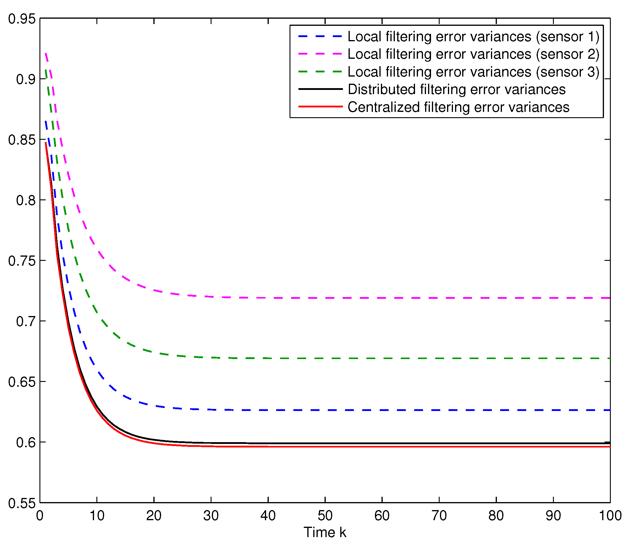
Performance of the local and fusion filtering algorithms. Let us assume that $\overline{\theta }=0.5$, and consider the same delay probabilities, ${\overline{\gamma }}^{\left(i\right)}=0.21$, for the three sensors obtained when ${\overline{\lambda }}^{\left(i\right)}=0.3$, $i=1,2$. In Figure 1, the error variances of the local, distributed and centralized filters are compared; this figure shows that the error variances of the distributed fusion filtering estimator are lower than those of every local estimator, but slightly greater than those of the centralized one. However, this slight difference is compensated by the fact that the distributed fusion structure reduces the computational cost and has better robustness and fault tolerance. Analogous results are obtained for other values of the probabilities $\overline{\theta }$ and ${\overline{\gamma }}^{\left(i\right)}$.

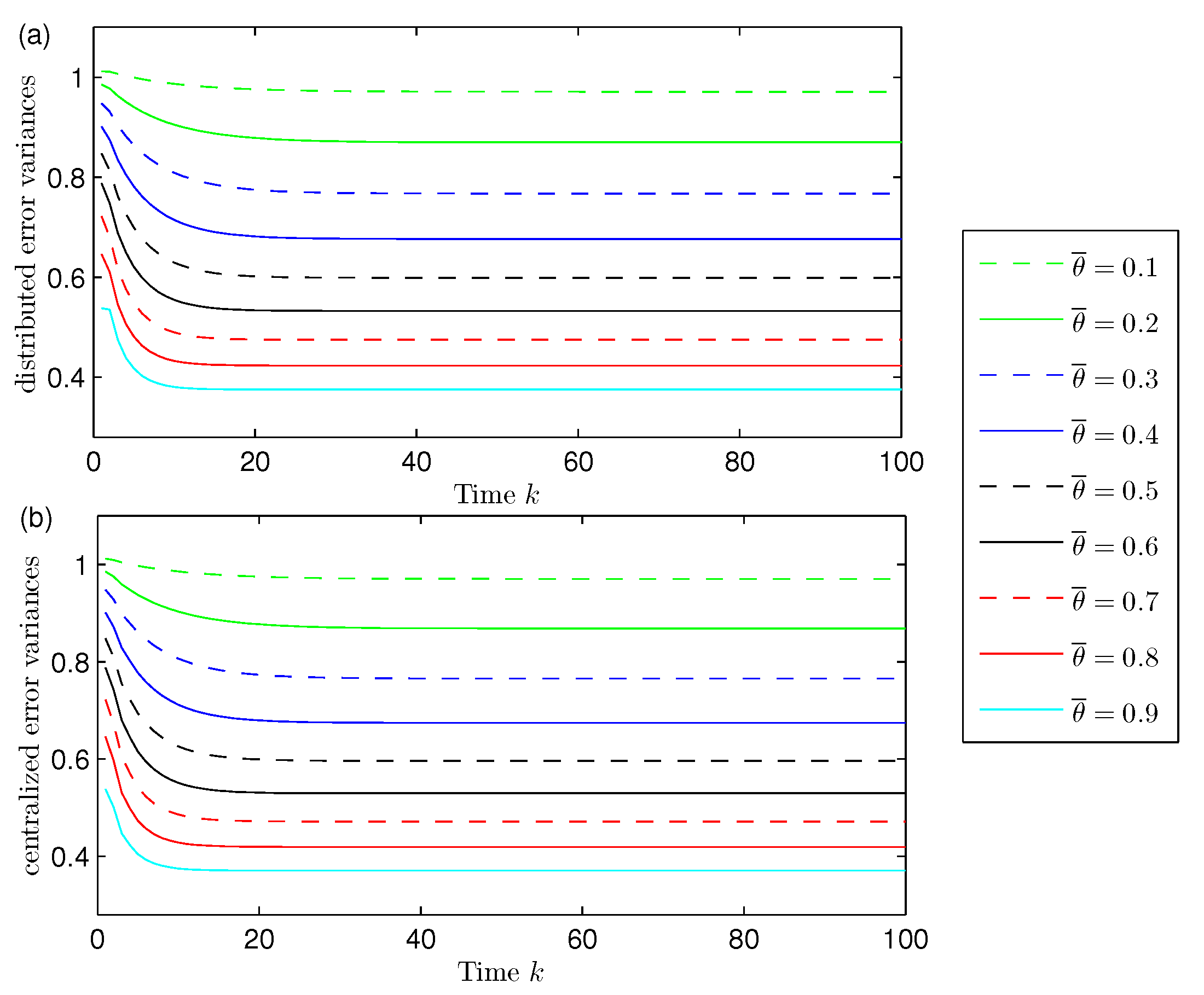
Influence of the missing measurements. Considering again ${\overline{\gamma }}^{\left(i\right)}=0.21$, $i=1,2,3$, in order to show the effect of the missing measurements phenomena, the distributed and centralized filtering error variances are displayed in Figure 2 for different values of the probability $\overline{\theta }$; specifically, when $\overline{\theta }$ is varied from 0.1 to 0.9. In this figure, both graphs (corresponding to the distributed and centralized fusion filters, respectively) show that the performance of the filters becomes poorer as $\overline{\theta }$ decrease, which means that, as expected, the performance of both filters improves as the probability of missing measurements, $1-\overline{\theta }$, decreases. This figure also confirms that both methods, distributed and centralized, have approximately the same accuracy for the different values of the missing probabilities, thus corroborating the previous comments.

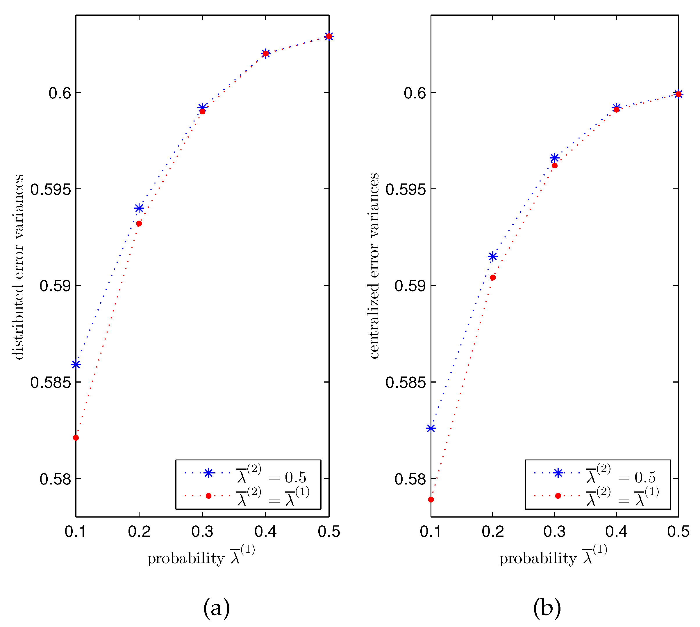
Influence of the transmission delays. For $\overline{\theta }=0.5$, different values for the probabilities ${\overline{\gamma }}^{\left(i\right)}$, $i=1,2,3$, of the Bernoulli variables modelling the one-step delay phenomenon in the transmissions from the sensors to the local processors have been considered to analyze its influence on the performance of the distributed and centralized fusion filters. Since the behavior of the error variances is analogous for all the iterations, only the results at a specific iteration ($k=100$) are displayed here. Specifically, Figure 3 shows a comparison of the filtering error variances at $k=100$ in the following cases:

(I)

Error variances versus ${\overline{\lambda }}^{\left(1\right)}$, when ${\overline{\lambda }}^{\left(2\right)}=0.5$. In this case, the values ${\overline{\lambda }}^{\left(1\right)}=0.1$, $0.2$, $0.3$, $0.4$ and $0.5$, lead to the values ${\overline{\gamma }}^{\left(1\right)}={\overline{\gamma }}^{\left(3\right)}=0.09,0.16,0.21,0.24$ and $0.25$, respectively, for the delay probabilities of sensors 1 and 3, whereas the delay probability of sensor 2 is constant and equal to $0.25$.

(II)

Error variances versus ${\overline{\lambda }}^{\left(1\right)}$, when ${\overline{\lambda }}^{\left(2\right)}={\overline{\lambda }}^{\left(1\right)}$. Now, as in Figure 2, the delay probabilities of the three sensors are equal, and they all take the aforementioned values.

Figure 3 shows that the performance of the distributed and centralized estimators is indeed influenced by the probability ${\overline{\lambda }}^{\left(i\right)}$ and, as expected, better estimations are obtained as ${\overline{\lambda }}^{\left(i\right)}$ becomes smaller, due to the fact that the delay probabilities, ${\overline{\gamma }}^{\left(i\right)}$, decrease with ${\overline{\lambda }}^{\left(i\right)}$. Moreover, this figure shows that the error variances in case (II) are less than those of case (I). This is due to the fact that, while the delay probabilities of the three sensors are varied in case (II), only two sensors vary their delay probabilities in case (I); since the constant delay probability of the other sensor is assumed to take its greatest possible value, this figure confirms that the estimation accuracy improves as the delay probabilities decrease.

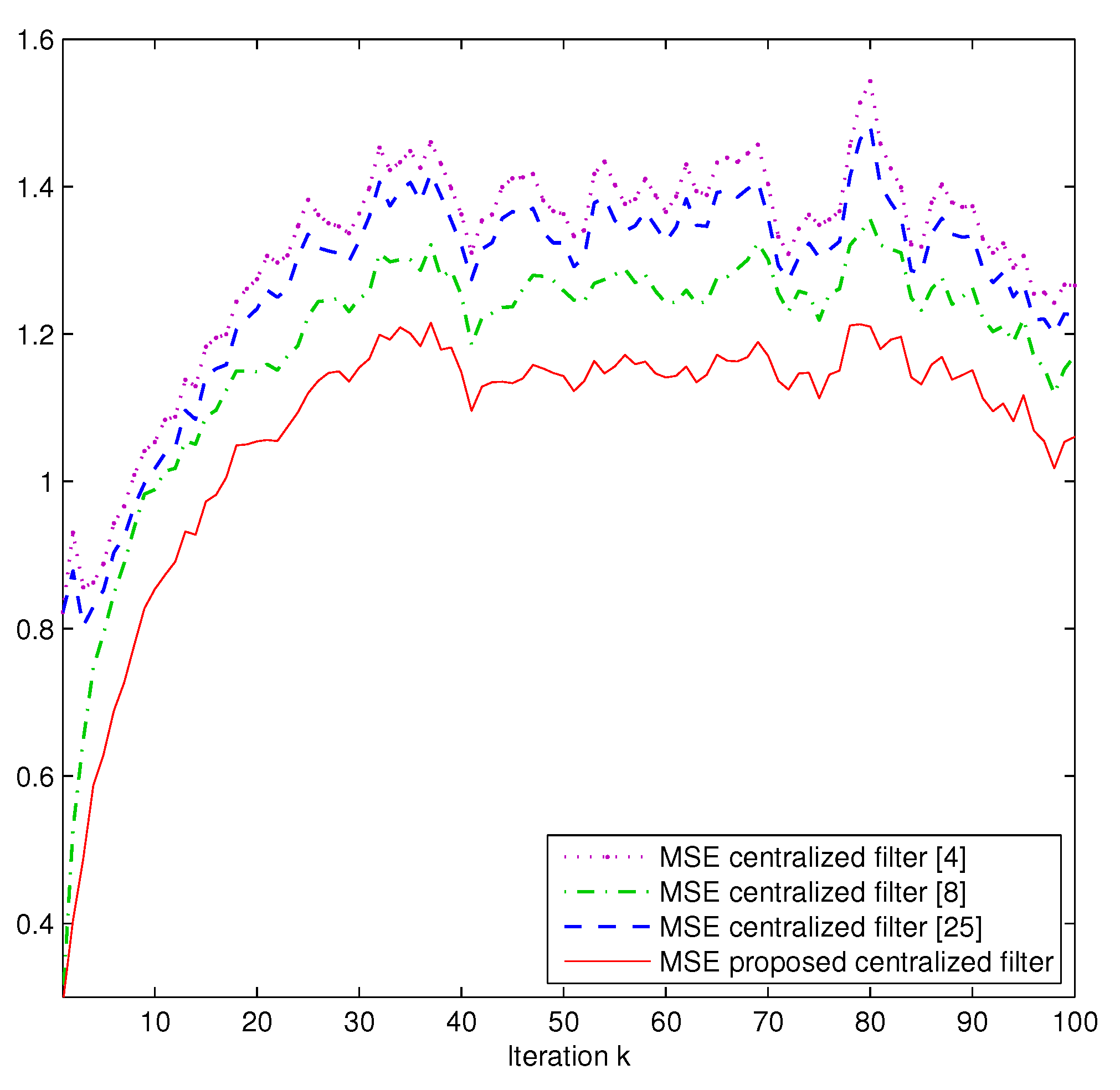
Comparison. Next, we present a comparative analysis of the proposed centralized filter and the following ones:

-

The centralized Kalman-type filter [4] for systems without uncertainties.

-

The centralized filter [8] for systems with missing measurements.

-

The centralized filter [25] for systems with correlated random delays.

Assuming the same probabilities $\overline{\theta }=0.5$ and ${\overline{\gamma }}^{\left(i\right)}=0.21$ as in Figure 1, and using one thousand independent simulations, the different centralized filtering estimates are compared using the mean square error (MSE) at each sampling time k, which is calculated as ${\displaystyle {\mathrm{MSE}}_k=\frac{1}{1000}\sum _{s=1}^{1000}{\left(x_k^{\left(s\right)}-{\widehat{x}}_{k/k}^{\left(s\right)}\right)}^2,}$ where $\left\{x_k^{\left(s\right)};1\le k\le 100\right\}$ denotes the s-th set of artificially simulated data and ${\widehat{x}}_{k/k}^{\left(s\right)}$ is the filter at the sampling time k in the s-th simulation run. The results are displayed in Figure 4, which shows that: (a) the proposed centralized filtering algorithm provides better estimations than the other filtering algorithms since the possibility of different simultaneous uncertainties in the different sensors is considered; (b) the centralized filter [8] outperforms the filter [25] since, even though the latter accommodates the effect of the delays during transmission, it does not take into account the missing measurement phenomenon in the sensors; (c) the filtering algorithm in [4] provides the worst estimations, a fact that was expected since neither the uncertainties in the measured outputs nor the delays during transmission are taken into account.

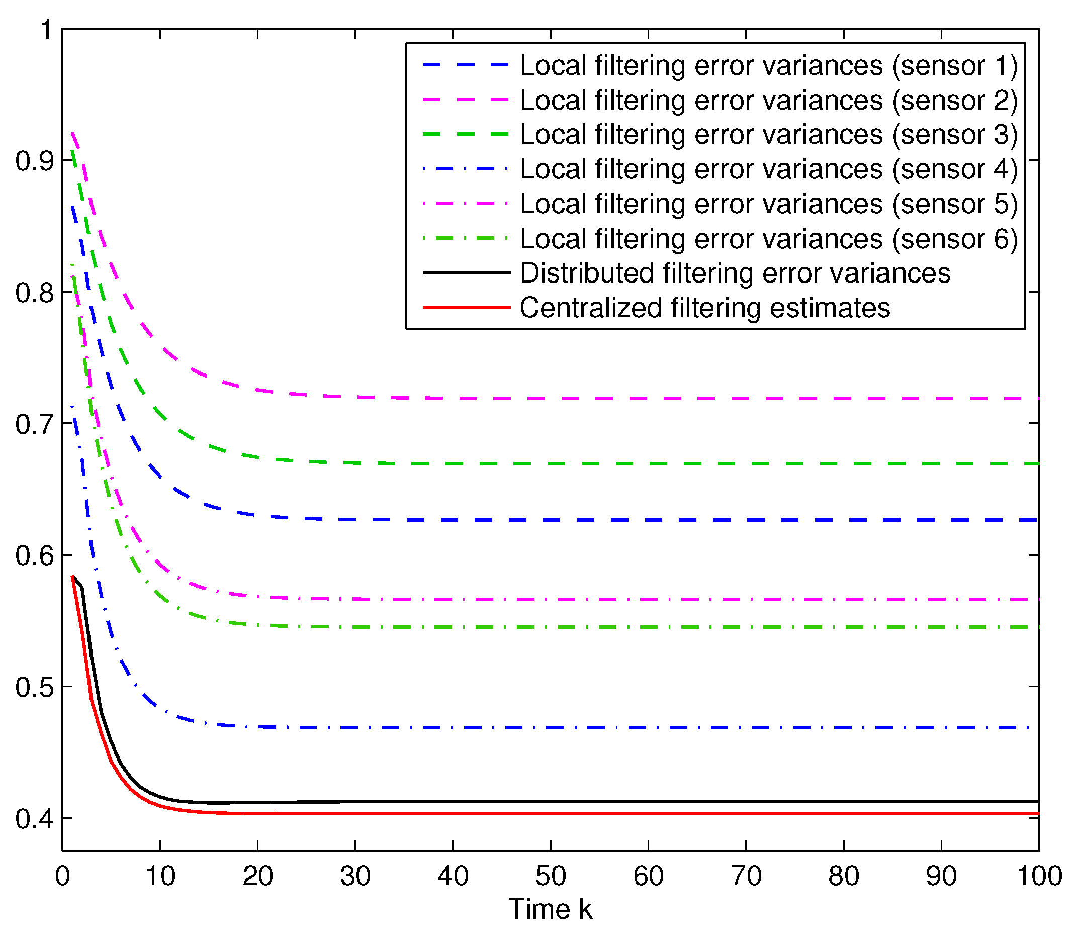
Six-sensor network. Finally, according to the anonymous reviewers suggestion, the feasibility of the proposed estimation algorithms is tested for a larger number of sensors. More specifically, three additional sensors are considered with the same characteristics as the previous ones, but a probability $\overline{{\theta }^{*}}=P({\theta }_k^{\left(i\right)}=1)=0.75$, $i=4,5,6$, for the Bernoulli random variables modelling the missing measurements phenomena. The results are shown in Figure 5, from which similar conclusions to those from Figure 1 are deduced.

6. Conclusions

In this paper, distributed and centralized fusion filtering algorithms have been designed in multi-sensor systems from measured outputs with both multiplicative and additive noises, assuming correlated random delays in transmissions. The main outcomes and results can be summarized as follows:

• Covariance information approach. The evolution model generating the signal process is not required to design the proposed distributed and centralized fusion filtering algorithms; nonetheless, they are also applicable to the conventional formulation using the state-space model.
• Measured outputs with multiplicative and additive noises. The sensor measured outputs are assumed to be affected by different stochastic uncertainties (namely, missing measurements and multiplicative noises), besides cross-correlation between the different sensor additive noises.
• Random one-step transmission delays. The fusion estimation problems are addressed assuming that random one-step delays may occur during the transmission of the sensor outputs through the network communication channels; the delays have different characteristics at the different sensors and they are assumed to be correlated and cross-correlated at consecutive sampling times. This correlation assumption covers many situations where the common assumption of independent delays is not realistic; for example, networked systems with stand-by sensors for the immediate replacement of a failed unit, thus avoiding the possibility of two successive delayed observations.
• Distributed and centralized fusion filtering algorithms. As a first step, a recursive algorithm for the local LS linear signal filter based on the measured output data coming from each sensor has been designed by an innovation approach; the computational procedure of the local algorithms is very simple and suitable for online applications. After that, the matrix-weighted sum that minimizes the mean-squared estimation error is proposed as distributed fusion estimator. Also, using covariance information, a recursive centralized LS linear filtering algorithm, with an analogous structure to that of the local algorithms, is proposed. The accuracy of the proposed fusion estimators, obtained under the LS optimality criterion, is measured by the error covariance matrices, which can be calculated offline as they do not depend on the current observed data set.