
The Catastrophe of Electric Vehicle Sales


Department of Mechanical Engineering, Stanford University, 496 Lomita Mall, Stanford, CA 94305, USA
Mathematics 2017, 5(3), 46; https://doi.org/10.3390/math5030046
Submission received: 9 August 2017
/
Revised: 30 August 2017
/
Accepted: 11 September 2017
/
Published: 17 September 2017
Abstract
:Electric vehicles have undergone a recent faddy trend in the United States and Europe, and several recent publications trumpet the continued rise of electric vehicles citing steadily-climbing monthly vehicle sales. The broad purpose of this study is to examine this optimism with some degree of mathematical rigor. Specifically, the methodology will use catastrophe theory to explore the possibility of a sudden, seemingly-unexplainable crash in vehicle sales. The study begins by defining optimal system equations that well-model the available sales data. Next, these optimal models are used to investigate the potential response to a slow dynamic acting on the relatively faster dynamic of the optimal system equations. Catastrophe theory indicates a potential sudden crash in sales when a slow dynamic is at-work. It is noteworthy that the prediction can be made even while sales are increasing.
1. Introduction
Worldwide electric car sales taken from U.S. Department of Energy data is to be investigated using Catastrophe Theory. Electric vehicle adoption is claimed to be gaining gradual momentum [1], but could this merely be hyped? An evaluation of electric vehicles’ market penetration scenarios [2] would seem to indicate the inevitability of ubiquitous use of electric vehicles. Nominal sales analysis methods [3] include period comparisons, break-even analysis, competitor sales analysis, year-over-year comparisons, and these methods normally use simple linear models. Since history has demonstrated that vehicle sales do not simply climb and fall linearly in accordance with low-order models, higher order assumptions must be evaluated. For a second-order or higher mathematical model, it is not guaranteed that the sales data will continue to climb. Instead, sales could suffer from catastrophe and plummet and go to a low or zero steady-state equilibrium value. Normally, Catastrophe Theory presumes the presence of fast and slow dynamics which can cause an otherwise stable system to experience discontinuous catastrophic “jumps”. The fast dynamic is modeled linearly with sufficient accuracy (often accuracy is increased with increasing model-order, as the higher order factors can account for the slow moving dynamic). The first step taken here is to use linear least squares to fit the data to an optimum linear mathematical model. The model is then extrapolated to visually see the steady-state behavior before formal stability analysis.
2. Catastrophe Theory
Catastrophe theory models the system using fast (dominant) linear dynamics plus slow dynamics whose combination result in real-world nonlinear affects that can often confound predication. The main point is that otherwise stable linear system models can be slowly changing such that they can rapidly become unstable (aka. “catastrophe”). The principle method of analysis is to differentiate the system equations and equate to zero to solve for equilibrium points. Next, each equilibrium point is evaluated as stable or unstable. Lastly, the system equation is slowly modified to see if any catastrophic “jump” occurs. If a jump occurs, the system can come to rest at a stable equilibrium point where sales have gone to zero (naturally, that is highly undesirable). Readers should be careful not to strongly claim that catastrophe will occur; however the results of such analysis should warn investors of the mathematical indications that catastrophe can occur, or perhaps more correctly catastrophe analysis indicates that sales crash will occur.
3. Results
We start by using least squares to find optimal system equations for increasingly higher order models (Figure 1). Sales data are compiled by Argonne’s Center for Transportation Research and reported to the U.S. Department of Energy’s Vehicle Technologies Office each month [4].
3.1. System Identification: Optimally Fitting Data to Assumed Models
Least squares
Figure 1 shows the least squares analysis based on cumulative vehicle sales.
3.2. Sales Rates from Differentiation of Assumed Models
Figure 2 displays the monthly sales raw data as points, and each subsequently higher-order model is displayed using a different type of line with each case displayed separately in Figure 3 for clarity. At initial glance, all the curves oscillate in a generally upward direction, so lacking further analysis, anticipating increasing sales (without a catastrophic jump) is a tempting conclusion.
3.3. Extrapolation by Forward Time Propagation
It is noteworthy to propagate the least squares system equations’ curves forward in time to see what nominal sales could be expected (Figure 4). The accuracy of optimal math models increased as the model order increased (i.e., the curves better fit the actual data). Data was available for 51 months (just over 4 years coinciding with the recent dramatic increase in gasoline prices), and models as high as sixth-order were investigated. It is noteworthy that recent data clearly reveals decreasing sales recently, coinciding with the dramatic reduction in gasoline prices accompanying the shale gas boom.
Extrapolation far beyond those 51 months (see Figure 4) revealed that all models except for the first order (linear) model experience catastrophic loss of sales (depicted) very quickly and did not recover for 20 years. The extrapolation was extended beyond 20 years (not depicted) revealing that sales would never recover. Thus, we see that all of the system equations of higher order (than the linear case) experience a dramatic steady fall in sales, while at least the 5th order case eventually rebounds dramatically after 221 months (in August 2029).
3.4. Equilibrium Point Analysis: Modeling Electric Car Sales with Catastrophe Theory: Fast and Slow Dynamics
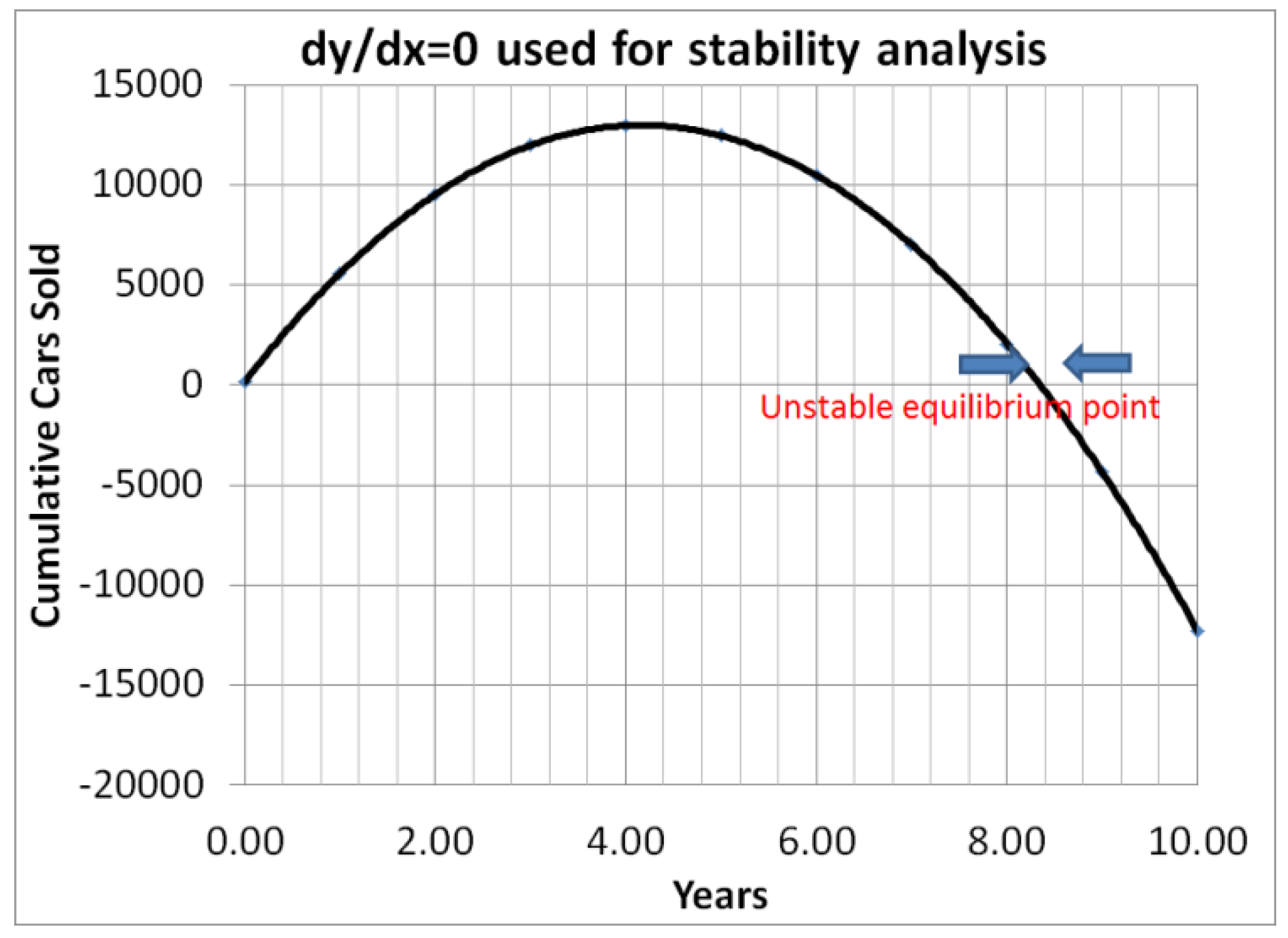
Continuing with our analysis, we investigate whether these system equations are susceptible to “jumps” associate with catastrophe theory. Differentiating the optimal system equations reveals potential equilibrium points in the system equation where the rate crosses zero (Figure 5). Furthermore we see that it is an unstable equilibrium point indicating potential catastrophe just shy of nine years in instances of slow dynamics.
3.5. Impulse Iteration: Analysis of System with Slow Moving Dynamic
Taking the third order case as an example (Equation (1)), we will differentiate, seeking equilibrium points for the general class of equations: where the final constant is chosen to fit the actual data at the initial time (i.e., x = 0). First, notice in the extrapolation of the system equations for both monthly and cumulative data seem to reveal sale will “crash” (Figure 6).
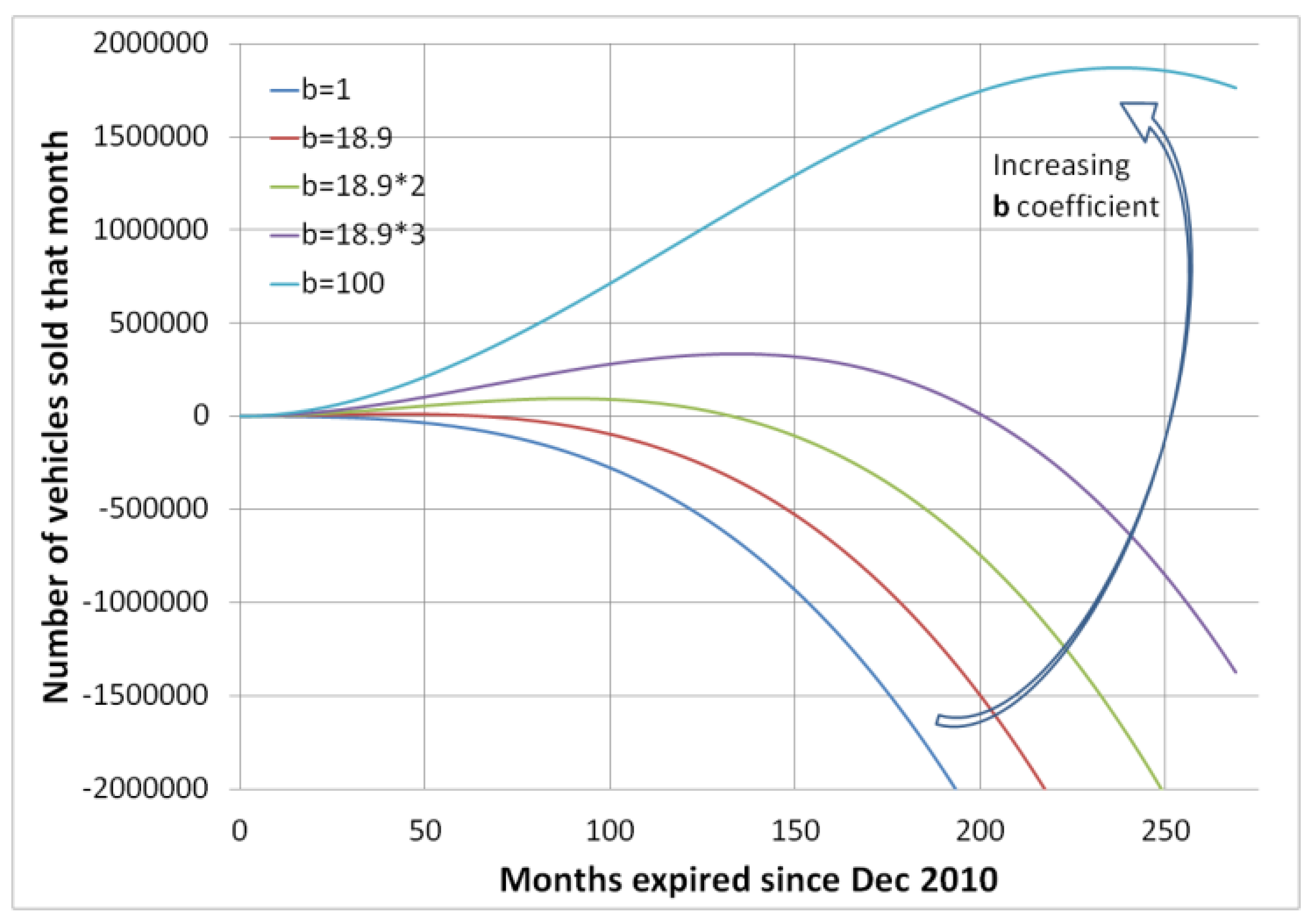
Iteration of coefficients reveals that modification between stable and unstable is best achieved by modifying the b coefficient on the squared-term. Before differentiating, the coefficients were chosen to match the least squares optimal system model, thus a = 0.2803, c = 73.886, and the final constant was set to 845.28 and b was iterated seeking improved performance. Control variables a, b, and c where investigated, and control variable b was found to have the most significant impact. Figure 7 depicts the least squares optimal system equation (b = 18.9) compared to higher and lower values of b. It is apparent that reducing b degrades sales and could be associated with higher gas prices. Lowering gas prices could be associated with increasing b which improves sales performance.
Next, y = −0.2803x3 + bx2 − 73.886x + 845.28 the least squares optimal system equation was differentiated seeking equilibrium points.
Equation (4) was plotted in Figure 8 for various choices of the b-coefficient revealing the impact of our choice on the potential for catastrophe in sales.
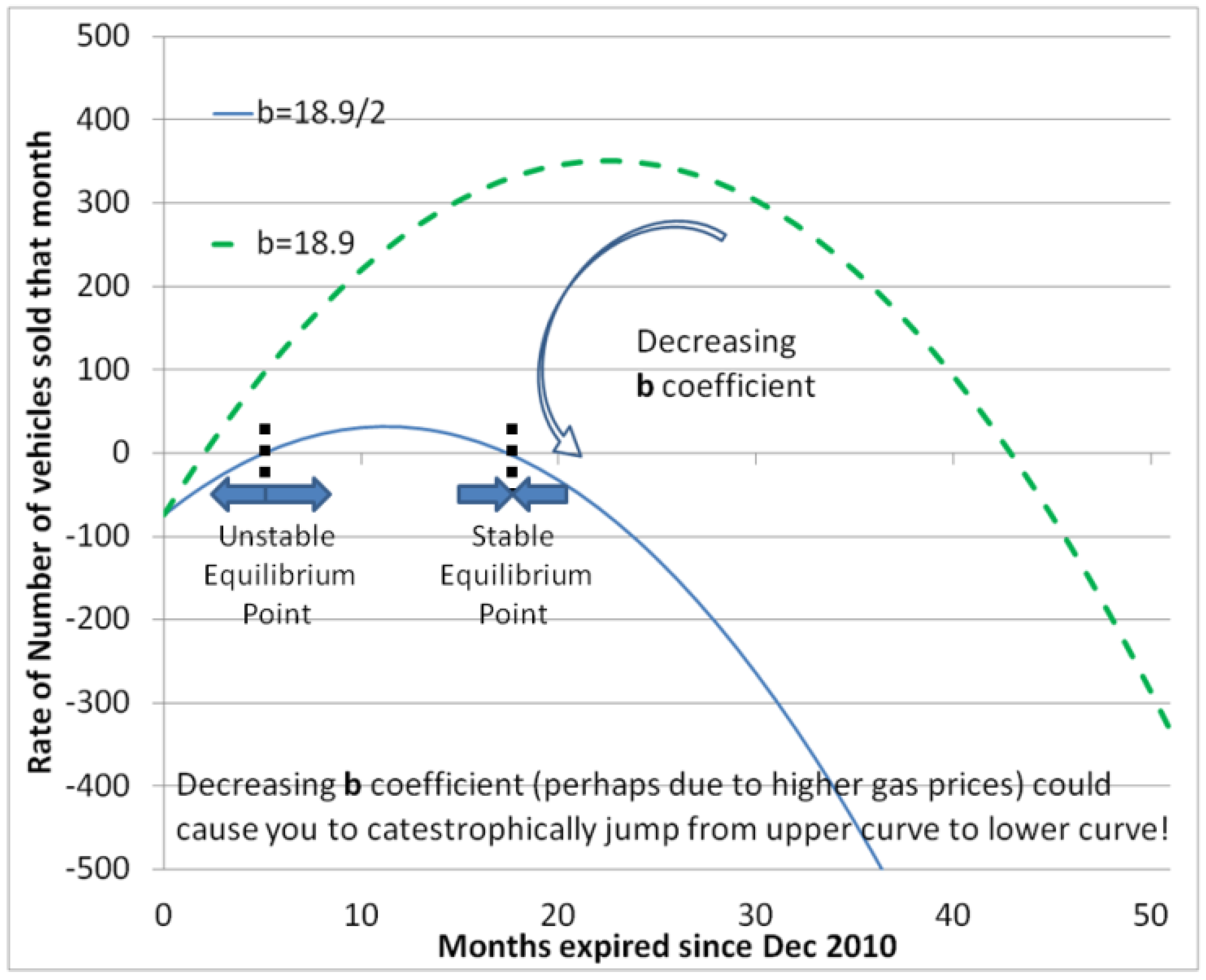
Using the iterated b values used earlier, the equilibrium points for each case occur when the derivative dy/dx = 0 (Figure 9). We see in all cases dy/dx > 0 at the start, but eventually go to zero and continue until dy/dx < 0. Next, consider what would happen if b decreases. Say, for instance you began on the nominal curve derived with least squares, but subsequently, the gas prices slowly, but steadily drop generating a decreasing b coefficient. When b was halved, you find yourself on the lower curve in Figure 9, and thus you would experience a catastrophic jump onto the lower curve which may have already passed through into the negative rate territory.
4. Discussion
The results show how catastrophe theory could provide prediction of a crash in electrical vehicle sales after experiencing the very beginning of a potential decline. In this study, seemingly good data that reflects a steady, oscillating climb in vehicle sales is used to predict a crash in monthly sales. Sometimes, slow moving dynamics applied to linear models is insufficient to indicate potential catastrophe, and in those cases subsequent analysis can include nonparametric regression methods such as kernel regression or smoothing splines in low-dimensional scenarios or for high-dimension data, additive models, multivariate adaptive regression splines, random forests, neural networks, and others might be used [5]. One particularly useful stochastic method for complex linear and nonlinear relationships simultaneously is called a “cusp catastrophe model”, where a high-order probability density function is used [6]. The cusp model has proven particularly effective for prediction in health behaviors. [7] These methods were not necessary to reveal the potential catastrophe in electric vehicle sales, but constitute interesting follow-on research for comparison with the results in this paper.
Conflicts of Interest
The authors declare no conflict of interest.
References
- E-Volution—Electric Vehicles in Europe: Gearing Up for a New Phase? Amsterdam Roundtables Foundation Report; McKinsey & Company: Amsterdam, The Netherlands, 2014.
- Nemry, F.; Brons, M. Plug-In Hybrid Scenarios of Electric Drive Vehicles; JRC Technical 222Notes; European Commission Joint Research Center Institute for Prospective Technological Studies: Luxembourg, 2010. [Google Scholar]
- Small Business Website. Hearst Newspapers, LLC. Available online: http://smallbusiness.chron.com/define-sales-analysis-5258.html (accessed on 30 August 2017).
- Argonne National Laboratory, Energy Systems. Light Duty Electric Drive Vehicle Monthly Sales Updates. Available online: https://www.anl.gov/energy-systems/project/light-duty-electric-drive-vehicles-monthly-sales-updates (accessed on 9 August 2017).
- Faraway, J.J. Extending the Linear Model with R: Generalized Linear Mixed-Effects and Nonparametric Regressionmodels; Chapman and Hall/CRC: Boca Raton, FL, USA, 2006. [Google Scholar]
- Zeeman, E.C. Catastrophe theory. Sci. Am. 1976, 234, 65–83. [Google Scholar] [CrossRef]
- Chen, D.G.; Lin, F.; Chen, X.J.; Tang, W.; Kitzman, H. Cusp Catastrophe Model: A Nonlinear Model for Health Outcomes in Nursing Research. Nurs. Res. 2014, 63, 211–220. [Google Scholar] [CrossRef] [PubMed]
Figure 1.
Least squares curves fitting cumulative sales data.
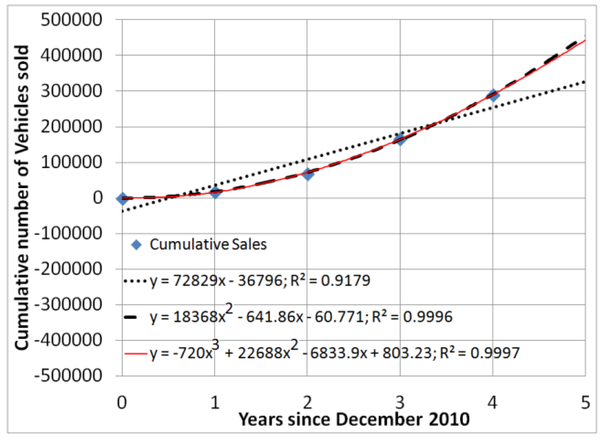
Figure 2.
Least squares curves (lines) fitting sales data (points).
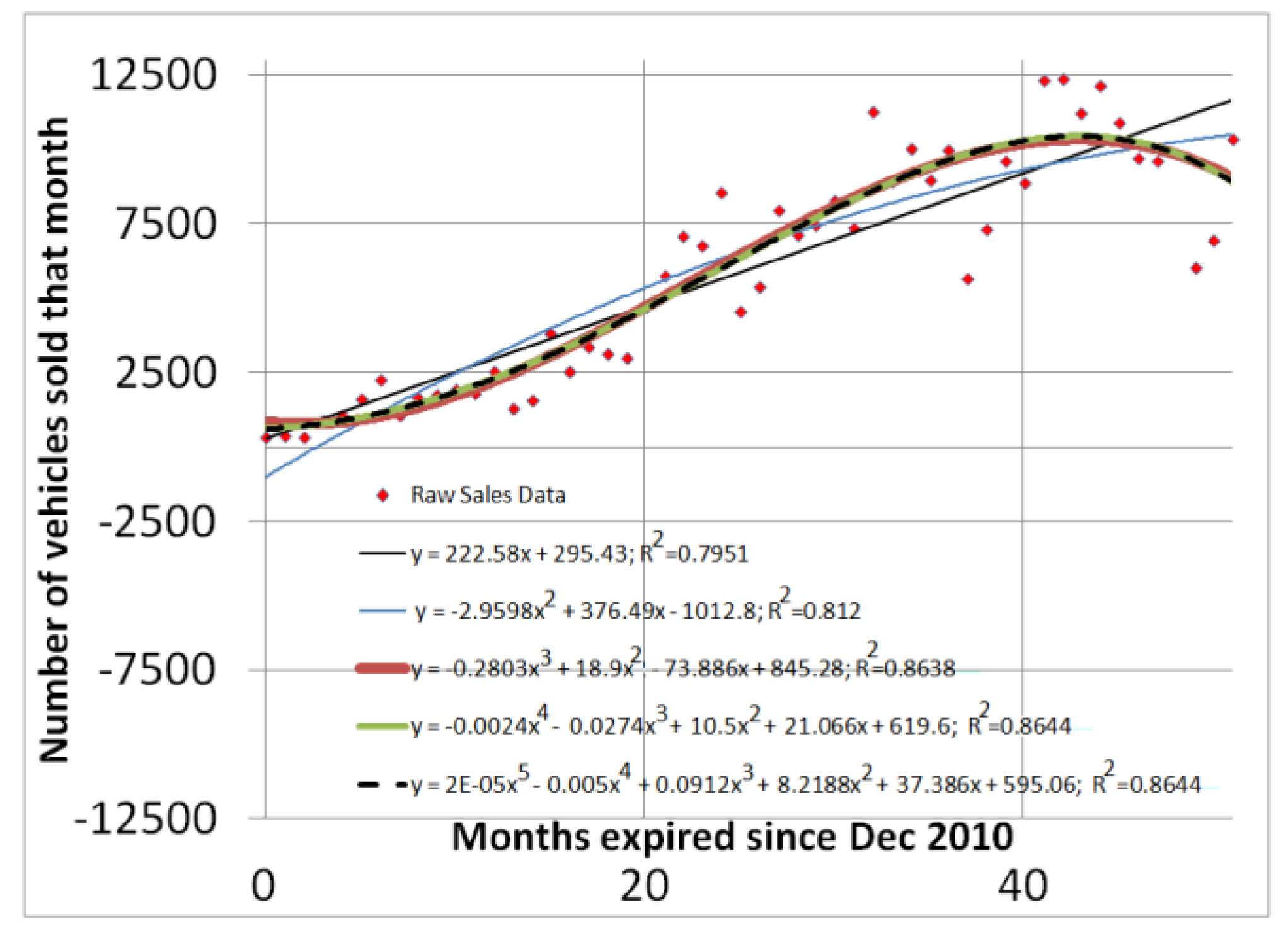
Figure 3.
Least squares curves (lines) fitting total monthly sales data (points): (a) first-order; (b) second-order; (c) third-order; (d) fourth-order; (e) fifth-order; (f) sixth-order model assumption.
Figure 3.
Least squares curves (lines) fitting total monthly sales data (points): (a) first-order; (b) second-order; (c) third-order; (d) fourth-order; (e) fifth-order; (f) sixth-order model assumption.

Figure 4.
Least Squares curves extrapolated to future-time.
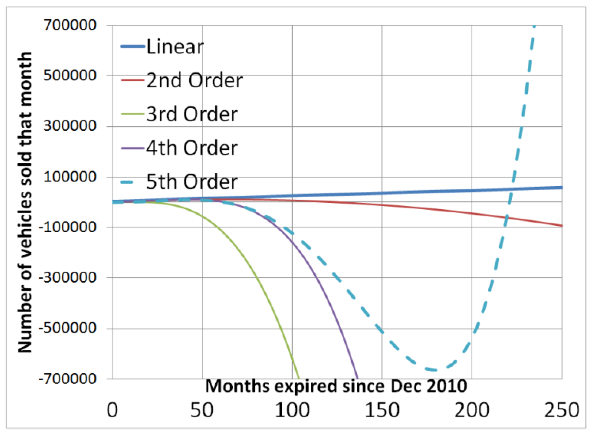
Figure 5.
Seek equilibrium points using dy/dx = 0.

Figure 6.
Extrapolation of system equations (sales and rate).
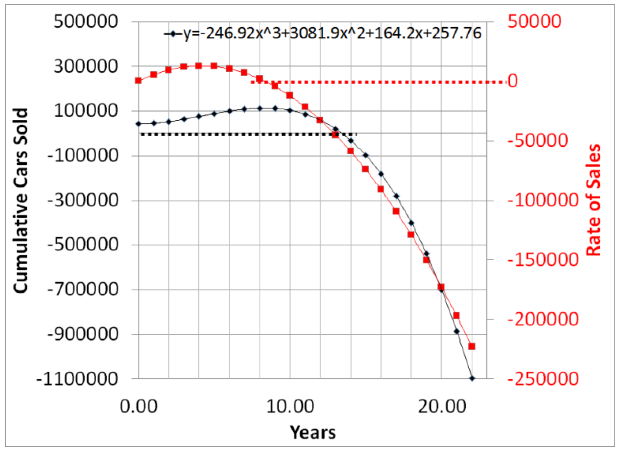
Figure 7.
Increasing b coefficient to increase sales.

Figure 8.
Increasing b coefficient to avoid stable equilibria.
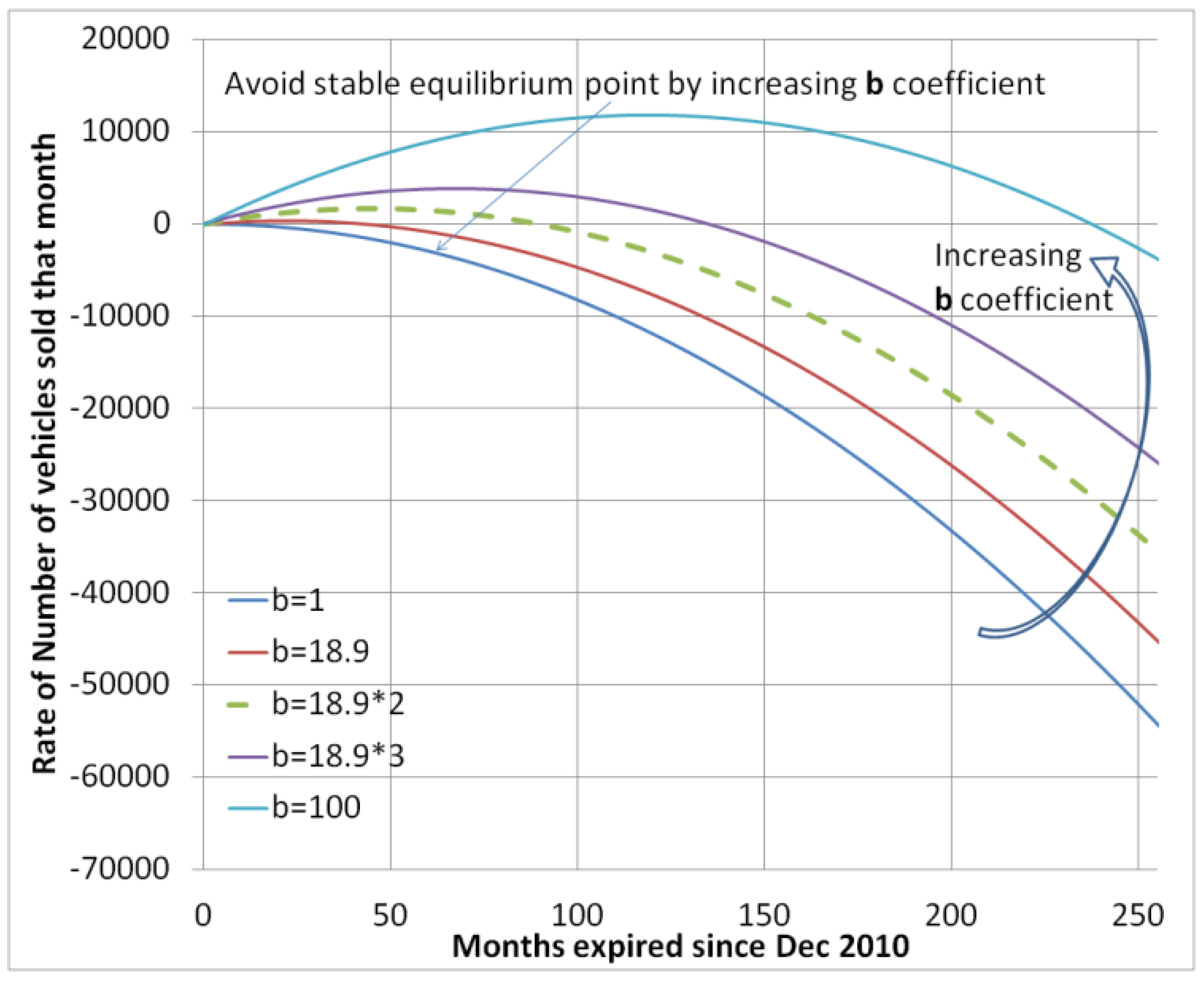
Figure 9.
Decreasing b coefficient could generate a “jump”.

© 2017 by the author. Licensee MDPI, Basel, Switzerland. This article is an open access article distributed under the terms and conditions of the Creative Commons Attribution (CC BY) license (http://creativecommons.org/licenses/by/4.0/).
Share and Cite
MDPI and ACS Style
Sands, T. The Catastrophe of Electric Vehicle Sales. Mathematics 2017, 5, 46. https://doi.org/10.3390/math5030046
AMA Style
Sands T. The Catastrophe of Electric Vehicle Sales. Mathematics. 2017; 5(3):46. https://doi.org/10.3390/math5030046
Chicago/Turabian StyleSands, Timothy. 2017. "The Catastrophe of Electric Vehicle Sales" Mathematics 5, no. 3: 46. https://doi.org/10.3390/math5030046
Note that from the first issue of 2016, this journal uses article numbers instead of page numbers. See further details here.