On the Achievable Stabilization Delay Margin for Linear Plants with Time-Varying Delays

College of Automation Engineering, Nanjing University of Aeronautics and Astronautics, 211106 Nanjing, China
Mathematics 2017, 5(4), 55; https://doi.org/10.3390/math5040055
Submission received: 24 September 2017
/
Revised: 19 October 2017
/
Accepted: 20 October 2017
/
Published: 25 October 2017
Abstract
:The paper contributes to stabilization problems of linear systems subject to time-varying delays. Drawing upon small gain criteria and robust analysis techniques, upper and lower bounds on the largest allowable time-varying delay are developed by using bilinear transformation and rational approximates. The results achieved are not only computationally efficient but also conceptually appealing. Furthermore, analytical expressions of the upper and lower bounds are derived for specific situations that demonstrate the dependence of those bounds on the unstable poles and nonminumum phase zeros of systems.
1. Introduction
Stability of time-delay systems has been long and well-studied for recent decades; nevertheless, the stabilization of time-delay systems proves a problem fundamentally more difficult, for which a satisfactory answer is yet to be available. Classic stabilization techniques include the time-domain approaches, involving with the solvability of algebraic riccati equations (AREs) or the feasibility of linear matrix inequalities) (LMIs) [1,2], the Smith predictor [3], the finite spectrum assignment [4], and the like. On the other hand, a robust stabilization problem draws more and more attention nowadays, allowing us to consider various classes of perturbations, such as time-varying type, with the aid of robust tools. There are two major approaches for robust stabilization. One is the time-domain approach, concerning the quadratic Lyapunov functions [5,6,7,8,9]. The other is the frequency-domain approach, employing the optimization tools (see [5,10,11,12,13,14], and the references therein). The existing results, however, have been largely focused on the synthesis issues. On the other hand, the results for fundamental robustness analysis are few. Moreover, the analysis on stabilizability is generally investigated case by case, without generalized solution.
In this paper, we are concerned with linear systems with an input time-varying delay
Let the time-varying delay be specified as
and
The purpose of this paper is to find a general method to determine the largest delay range such that there exists an LTI feedback controller that can stabilize the system (1) through the output feedback
for all time-varying delays that satisfy Label (2). The feedback configuration is shown in Figure 1, where represents the linear operator
The problem on stabilization delay margin has been under investigation for some time. In [2] (p. 154), the delay margin was examined for the first-order system with a constant delay stabilized by static feedback, while in [15], the stabilization was achieved by using PID controllers for first-order systems. Furthermore, for single-input single-output (SISO) systems with constant delays, the upper bound was determined in [16,17] for general LTI systems with an arbitrary number of unstable poles. These bounds consequently provide a limit beyond which no single LTI output feedback controller may exist to robustly stabilize a delay plant family within the delay margin. On the other hand, lower bounds on the delay margin were developed by the authors in [18], which provide instead, an interval of the delay range ensuring that the delayed plant can be robustly stabilized for SISO systems with constant delays and the possibility that the lower bounds can be extended to LTI systems with time-varying delays.
In this paper, we seek to explore both the upper and lower bounds on the delay margin for LTI systems with time-varying delays and investigate the optimal controller synthesis problem in this paper. This development is nontrivial. It appears that, in all cases, our results not only are computationally attractive, but shed significant conceptual insights; furthermore, our developments generate analytical expressions for specific plants, such as systems with one unstable pole or one nonminimum phase zero, revealing how fundamentally unstable poles and nonminimum phase zeros may limit the range of delays over which a plant may or may not be stabilized. In addition, the optimal feedback controller can be obtained by solving the control problem. The results can be applied directly to SISO systems subject to time-varying delays and extended to multiple-input multiple-output (MIMO) systems with time-varying delays.
We end this section with a brief description on the notation. Let be the space of real numbers, the space of n-dimensional real vectors, and the n-dimensional space of positive real numbers. Let , , and be the open left and the open right-half of the complex plane, and the closed right-half of the complex plane, respectively. denotes the conjugate of a complex number z, and denotes the conjugate transpose of a complex vector x, while denotes the conjugate transpose of a complex matrix A. We denote the largest real eigenvalue of a matrix A by , and for a Hermitian matrix A, its largest eigenvalue is denoted by . or means that A is nonnegative definite or positive definite. For any stable transfer function matrix , define its norm by
where denotes the largest singular value. For an n-tuple of scalars, vectors and matrices with compatible dimensions, we denote
2. Problem Formulation
Before dealing with the robust stabilization analysis for LTI systems with time-varying delays, we focus on the stabilization delay margin problem under the constant delay situation firstly. Consider the feedback system depicted in Figure 2, where denotes a family of plants with an unknown constant delay , and denotes the delay-free plant
Suppose that can be robustly stabilized by some finite-dimensional LTI controller . Hence, the same controller can thus stabilize for sufficiently small by continuity. The delay margin problem concerns the fundamental limit on robust stabilization of systems with time delays, i.e., what is the largest delay such that there exists a certain LTI controller that can stabilize all the plants within that range? In other words, the delay margin problem seeks to determine the largest delay range within which can be stabilized by a finite-dimensional LTI controller , or equivalently, the endpoint of delay range where the delay plan cannot be robustly stabilized by a single, fixed controller. Therefore, the problem amounts to computing
or, alternatively,
For to stabilize the delayed plant (4), it is both necessary and sufficient that
Since can be stabilized by , the above condition is equivalent to
where is the system’s complementary sensitivity function. Thus, the delay margin problem is equivalent to find
Since the exact delay margin is difficult to achieve, an alternative way is to estimate the upper bound and lower bound of the delay margin. Evidently, . Based on a small gain theorem, there exists some stabilizing for all if
Hence, a sufficient condition is obtained that provides a computing method on the lower bound of the delay margin. Similarly, there exists no controller to stabilize if for any such that
In other words, the upper bound of the delay margin can be calculated according to the following condition. The plant can not be stabilized by any controller if with
3. Main Results
3.1. Upper Bounds on the Delay Margin
Consider the time-varying delay system (1). It is easy to see that the upper bound for the constant delay case is also an upper bound on h, i.e., . Consequently, the main point is to compute by conditions (8) and (9). However, it is still difficult compute since the all-pass function is irrational. Thus, it is useful to use another all-pass and rational function to estimate . In this paper, we use bilinear transformation to estimate the upper bound.
Define an all-pass function Note that . Then, for any , let
Since we have
Define Then, the following conditions are satisfied
where p is the unstable pole of the delay-free plant . Note that condition (12) holds due to the interpolation . By continuity, we have
Referring to condtion (9), it can be concluded that the nominal plant is stabilizable for all . Hence, we are led to the following lemma.
Lemma 1.
Suppose that has only one unstable pole , and no nonminimum phase zero. Then, there exists no controller that can stabilize the system (4) for all with
Moreover, if has multiple unstable poles , , and no mominimum phase zero. Then,
Additionaly, suppose also that has one unstable pole , and one nominimum phase zero . If , then there exists no controller that can stabilize the system (4) for all with
Proof.
By bilinear transformation, is equal to as long as . Let , condition (13) turns to be
Upon Label (9), the upper bound can be obtained as Label (14) only has one unstable pole. The upper bound (15) can be derived in the similar manner. On the other hand, under the circumstance that has one unstable pole and one nominimum phase zero, the bilinear transformation function is chosen to be
by noting that For any , let
which gives rise to
Define Analogously, the upper bound (16) can be easily obtained. ☐
In what follows, we shall extend our results on upper bounds of delay margin to LTI systems with time-varying delays. The following theorem is an easy consequence of Lemma 1. Evidently, if no controller may exist to robustly stabilize a plant with a constant delay beyond the range of delay margin, then no controller may achieve the same for plants subject to time-varying delays.
Theorem 1.
Let be a real unstable pole of . Then, there exists no controller that can stabilize the system (1) subject to (2) if
Note that the upper bound of the delay margin only involves with the delay bound h, which implies the time-varying delay may vary arbitrarily fast, as long as it is bounded by some certain value.
3.2. Lower Bounds on the Delay Margin
In the following part, we work to find an LTI controller such that the delay system (1) is stabilized by way of the output feedback within a region defined by ().
By model transformation, it is possible to employ the approximations of the time-varying operator
i.e.,
where I is the identity operator. Then, the original system (1) can be regarded as Figure 3. In view of the small gain theorem [19], system (1) subject to Labels (2) and (3) is stable if
with and being the certain and uncertain part, respectively.
It is worth noting that the original system (1) with the controller in Figure 1 is stable whenever the system depicted in Figure 3 is stable [1]. Let be the transfer function of the delay-free plant. It is then useful to estimate the induced norm of the uncertainty . One such estimate can be obtained by employing the Littlewood’s Second Principle. An approximation in this spirit was developed in [20].
Proof.
Let be an arbitrary small subset of the interval . Assume that a real-valued function with can be approximated well by some function with . Thus, the Fourier transform of of should satisfy
with It is evident that
which can be further extended to be
by constructing a positive function such that
We note that
As such, Inequality (26) is equivalent to
where can be arbitrarily small.
Next, we concern the estimation of . Recalling Label (24), we can express by the following sink function
satisfying
Define . Then, its Fourier transform satisfies
Thus, can be estimated by with sufficient small . Let and . We can rewirte as
with
Consequently,
Define
Thus, we can rewrite Equation (32) to be
We then estimate the norm of , and one by one. Since that can be expressed as
the norm bound of can be obtained as follows
where the last inequality is derived in light of (31).
Concerning is arbitrarily small (i.e., b is arbitrary small) and we are led to
and
As a result,
In other words, is bounded by
Upon above, condition (21) is equivalent to
for sufficiently small . Construct a parameter-dependent rational approximation
such that
Since can be selected to be arbitrarily small, condition (39) is satisfied whenever
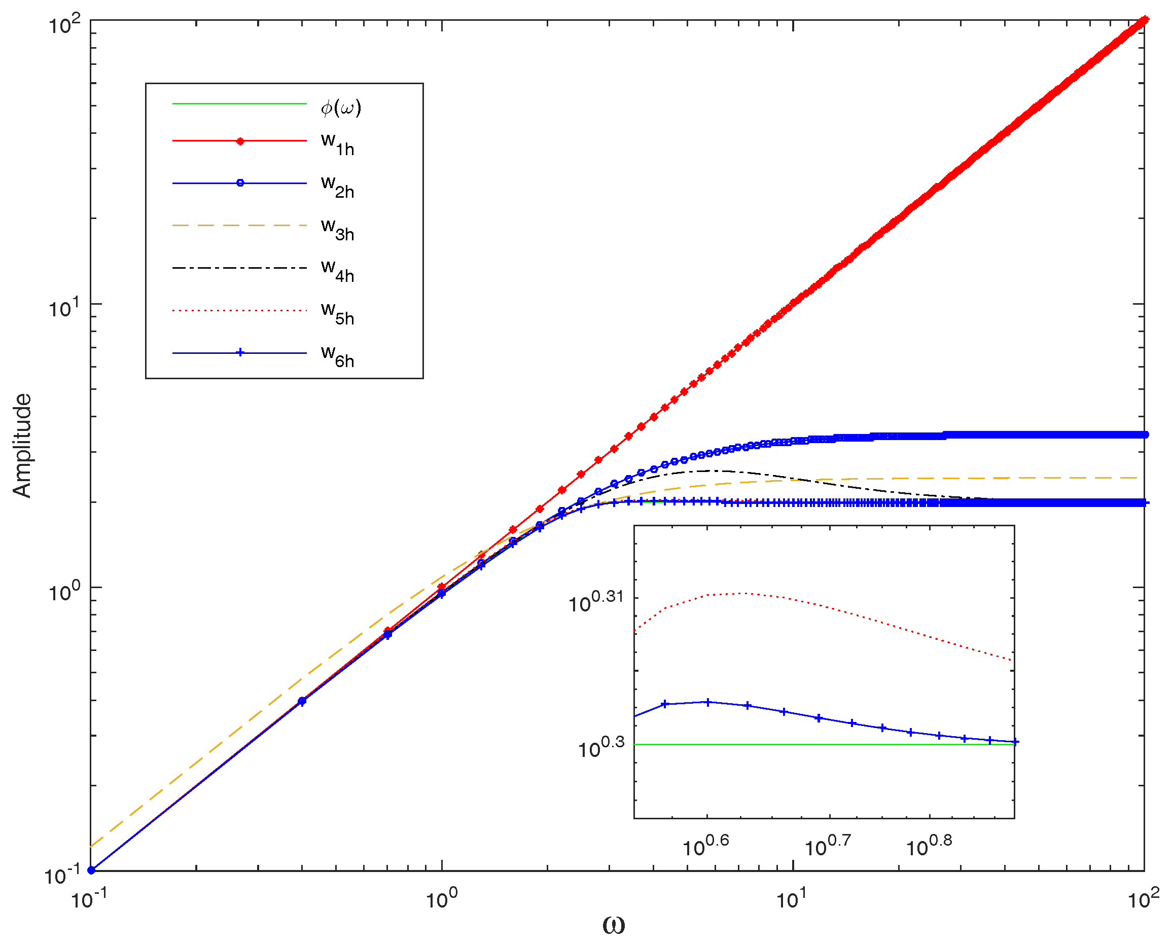
We require that be stable and has no nonminimum phase zero, excluding the origin where might have a zero, that is, . This latter condition may be imposed to ensure a close-fit of to at low frequencies. Without losing any generality, we let for , and for . The following are some specific approximants obtained in, e.g., [21,22,23]:
and
The frequency responses of these candidates are shown in Figure 4, from which we can conclude that approximates better one after one with the higher function order. By solving the optimization problem in Label (42), a lower bound h on the delay margin can be derived that will guarantee the existence of a stabilizing controller for system (1) with all subject to Labels (2) and (3).
Since h corresponds to an optimal optimization problem, this robustly stabilizing controller can be synthesized accordingly. Indeed, to synthesize this robustly stabilizing controller , it suffices to solve the standard control problem in Label (42), which gives rise an optimal controller K(s) depending on h. In this vein, it is worth pointing out that a lower order , such as those given in Label (43)–(48), can be particularly desirable, since they potentially result in low-order controllers. We shall demonstrate this point explicitly in the numerical example.
The following lemma, adopted from [24,25], is concerned with the Nevanlinna–Pick tangential interpolation problem, providing an essential tool converting the computation into the analytical interpolation.
Lemma 3.
Let and denote distinct points with for any i and j. Consider a rational matrix function , satisfying
for some vectors and with compatible dimensions. Then, is stable and if and only if
with
Theorem 2.
Proof.
The proof follows directly from Lemma 3, together with Label (42). ☐
To put it simply, analytical bounds can be obtained for some specific cases.
Corollary 1.
Consider the delay free plant with one unstable pole and one nonminimum phase zero . Let be stabilized by some . Then, for satisfying Label (41), system (1) subject to Labels (2) and (3) can be stabilized by some with () is the solution of
In particular, if given in Labels (43)–(46), , for , we have:
- (1)
- (2)
- (3)
- (4)
Moreover, consider the delay free plant with one unstable pole , and distinct nonminimum phase zeros . Let be stabilized by some . Then, for satisfying (41), system (1) subject to Labels (2) and (3) can be stabilized by some with () is the solution of
In particular, if given in Labels (43)–(46), , for , we have:
- (1)
- (2)
- (3)
- (4)
Note that, for , h recovers essentially the delay margin obtained for LTI systems with a constant unknown delay [18].
4. Illustrative Example
Example 1.
Consider the following system with a time-varying delay
The transfer function of the delay-free plant is
with two unstable poles, , and . Suppose that the input is a square wave signal, given by , and the time-varying delay is
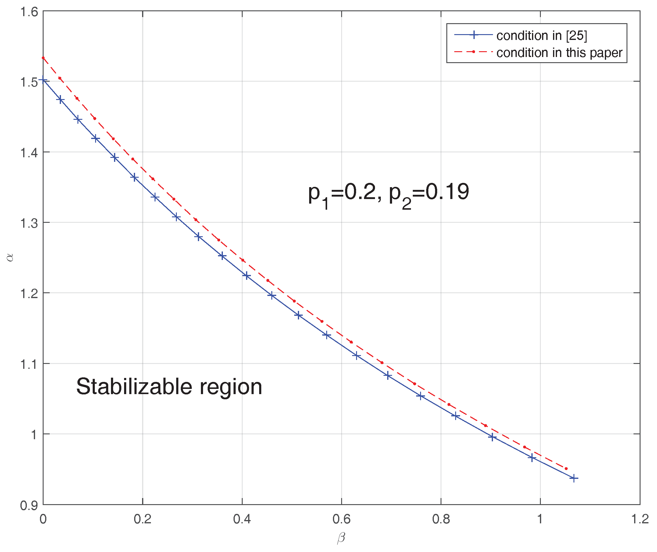
Then, the maximal delay range and variation rate are and The upper bound of the delay margin can be computed to be by Theorem 1, which means that there exists no controller that can stabilize system (50) with time-varying delay (51) if . On the other hand, the lower bound can be calculated according to Theorem 2. Figure 5 shows that our stabilizable region in terms of of improves that in [23].
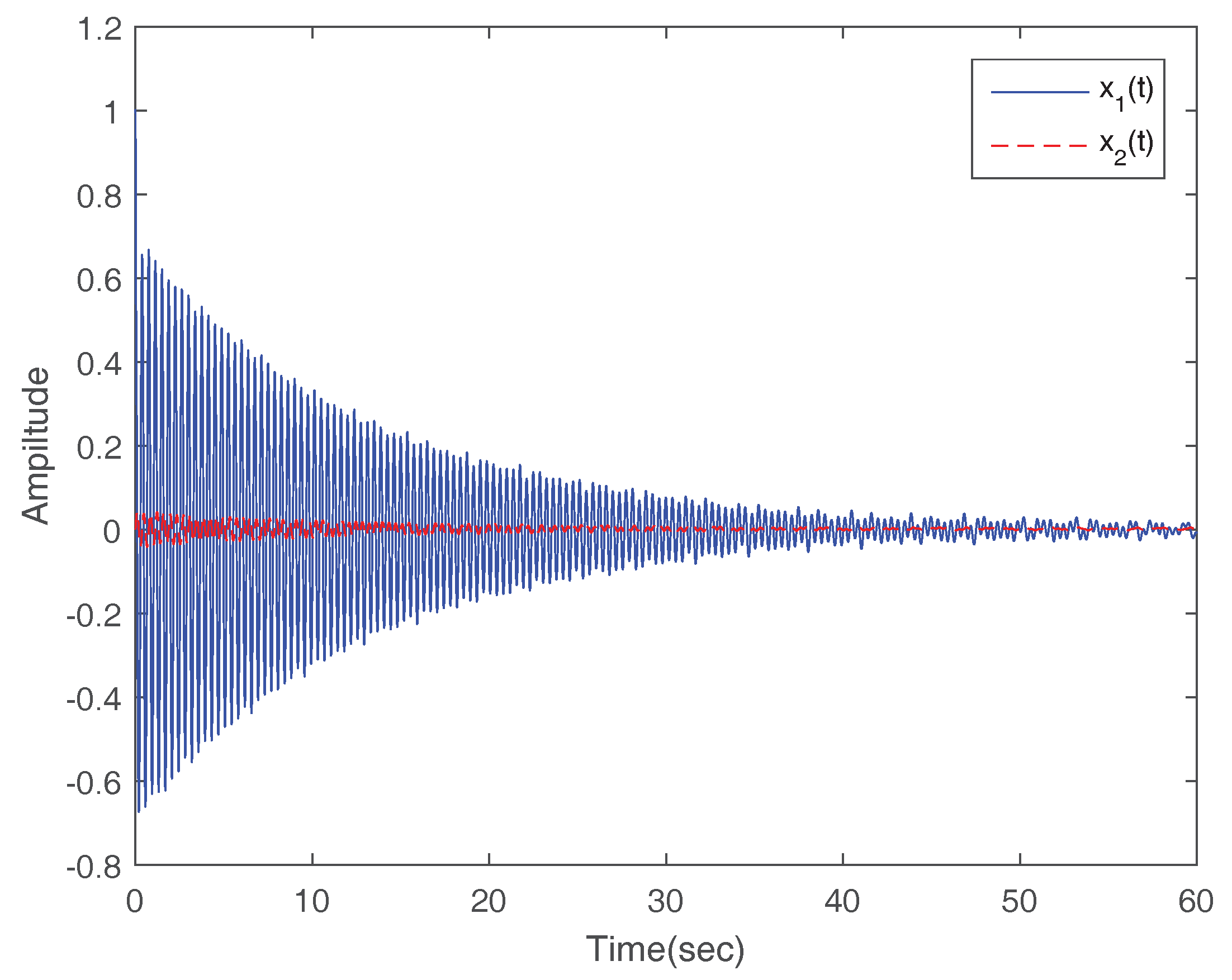
Let us then consider a specific delay function with , ; that is,
Since lies in the stabilizability region, system (50) can be stabilized by some controller ; indeed, the optimal controller can be found by solving the control problem in Label (42) with rational approximant in Label (48), as
Figure 6 exhibits a stable state response, where the system is excited by the unit step input .
5. Conclusions
In this paper, we develop readily computational upper and lower bounds on the robust stabilization margin for LTI systems with time-varying delays. By employing a bilinear transformation, the upper bounds for systems with constant delays are extended to systems with time-varying delays, while the lower bounds are investigated by means of analytical interpolations and rational approximations. Moreover, our results yield analytical expressions for more specific plants, such as systems with unstable poles and nonminimum phase zeros, demonstrating the significant dependencies of the upper and lower stabilization bounds on those poles and zeros. Furthermore, the optimal stabilizing controller can be obtained directly from our stabilization conditions. These results are efficiently computable, less conservative and conceptually appealing, which can be applied directly to SISO systems, while the delay region can be estimated by solving an LMI problem for MIMO systems with time-varying delays.
Acknowledgments
This research was supported by Natural Science Foundation of China under the grant 61603179, China Postdoctoral Science Foundation under the grant 2016M601805 and Fundamental Research Funds for the Central Universities under grant NJ20170005.
Conflicts of Interest
The authors declare no conflict of interest.
References
- Gu, K.; Kharitonov, V.; Chen, J. Stability of Time-Delay Systems; Bitkhäuser: Boston, MA, USA, 2003. [Google Scholar]
- Michiels, W.; Niculescu, S.-I. Stability and Stabilization of Time-Delay Systems: An Eigenvalue-Based Approach; Society for Industrial and Applied Mathematics (SIAM): Philadelphia, PA, USA, 2007. [Google Scholar]
- Palmor, Z.J. Time-delay compensation: Smith predictor and its modifications. In The Control Handbook; Levine, W.S., Ed.; CRC Press: Boca Raton, FL, USA, 1996; pp. 224–237. [Google Scholar]
- Manitius, A.Z.; Olbrot, A.W. Finite spectrum assignment problem for systems with delays. IEEE Trans. Autom. Control 1979, 24, 541–552. [Google Scholar] [CrossRef]
- Anderson, B.; Moore, J.B. Optimal Control: Linear Quadratic Methods; Prentice-Hall, Inc.: Upper Saddle River, NJ, USA, 1990. [Google Scholar]
- Khargonekar, P.P.; Petersen, I.R.; Zhou, K. Robust stabilization of uncertain linear systems: Quadratic stabilizability and H∞ control theory. IEEE Trans. Autom. Control 1990, 35, 356–361. [Google Scholar] [CrossRef]
- Barmish, B.R. Necessary and sufficient conditions for quadratic stabilizability of an uncertain system. J. Optim. Theory Appl. 1985, 46, 399–406. [Google Scholar] [CrossRef]
- Petersen, I.R.; Hollot, C.V. A riccati equation approach to the stabilization of uncertain linear systems. Automatica 1986, 22, 397–411. [Google Scholar] [CrossRef]
- Petersen, I.R. A stabilization algorithm for a class of uncertain linear systems. Syst. Control Lett. 1987, 8, 351–357. [Google Scholar] [CrossRef]
- Doyle, J.C.; Glover, K.; Khargonekar, P.P.; Francis, B.A. State-space solutions to standard H2 and H∞ control problems. IEEE Trans. Autom. Control 1989, 34, 831–847. [Google Scholar] [CrossRef]
- Francis, B.A. A Course in H∞ Control Theory; Springer: Berlin, Germany, 1987. [Google Scholar]
- Niculescu, S.-I. H∞ memoryless control with an α-stability constraint for time-delay systems: An LMI approach. IEEE Trans. Autom. Control 1998, 43, 739–743. [Google Scholar] [CrossRef]
- Zhou, K.; Doyle, J.C.; Glover, K. Robust and Optimal Control; Prentice-Hall: Upper Saddle River, NJ, USA, 1996. [Google Scholar]
- Briat, C. Robust stability and stabilization of uncertain linear positive systems via integral linear constraints: L1-gain and L∞-gain characterization. Int. J. Robust Nonlinear Control 2014, 23, 1932–1954. [Google Scholar] [CrossRef]
- Silva, G.J.; Datta, A.; Bhattacharyya, S.P. New results on the synthesis of PID controllers. IEEE Trans. Autom. Control 2002, 47, 241–252. [Google Scholar] [CrossRef]
- Middleton, R.H.; Miller, D.E. On the achievable delay margin using LTI control for unstable plants. IEEE Trans. Autom. Control 2007, 52, 1194–1207. [Google Scholar] [CrossRef]
- Ju, P.; Zhang, H. Further results on the achievable delay margin using LTI control. IEEE Trans. Autom. Control 2016, 61, 3134–3139. [Google Scholar] [CrossRef]
- Qi, T.; Zhu, J.; Chen, J. Fundamental Limits on Uncertain Delays: When Is a Delay System Stabilizable by LTI Controllers? IEEE Trans. Autom. Control 2017, 62, 1314–1328. [Google Scholar] [CrossRef]
- Zhu, J.; Chen, J.; Qi, T. Small-gain stability conditions for linear systems with time-varying delays. In Proceedings of the 2013 American Control Conference, Washington, DC, USA, 17–19 June 2013; pp. 1757–1762. [Google Scholar]
- Kao, C.Y.; Rantzer, A. Stability analysis of systems with uncertain time-varying delays. Automatica 2007, 43, 959–970. [Google Scholar] [CrossRef]
- Wang, Z.Q.; Lundstrom, P.; Skogestad, S. Representation of uncertain time delays in the H∞ framework. Int. J. Control 1994, 59, 627–638. [Google Scholar] [CrossRef]
- Huang, Y.; Zhou, K. Robust stability of uncertain time delay systems. IEEE Trans. Autom. Control 2000, 45, 2169–2173. [Google Scholar] [CrossRef]
- Zhu, J.; Qi, D. Robust stabilizability of linear plants with time-varying delays. In Proceedings of the 2016 IEEE Chinese Guidance, Navigation and Control Conference, Nanjing, China, 12–14 August 2016; pp. 2064–2069. [Google Scholar]
- Ball, J.A.; Gohberg, I.; Rodman, L. Interpolation of Rational Matrix Functions; Birkhäuser: Basel, Switzerland, 1990. [Google Scholar]
- Chen, J. Logarithmic integrals, interpolation bounds, and performance limitations in mimo feedback systems. IEEE Trans. Autom. Control 2000, 45, 1098–1115. [Google Scholar] [CrossRef]
Figure 1.
Feedback system with time-varying input delay.
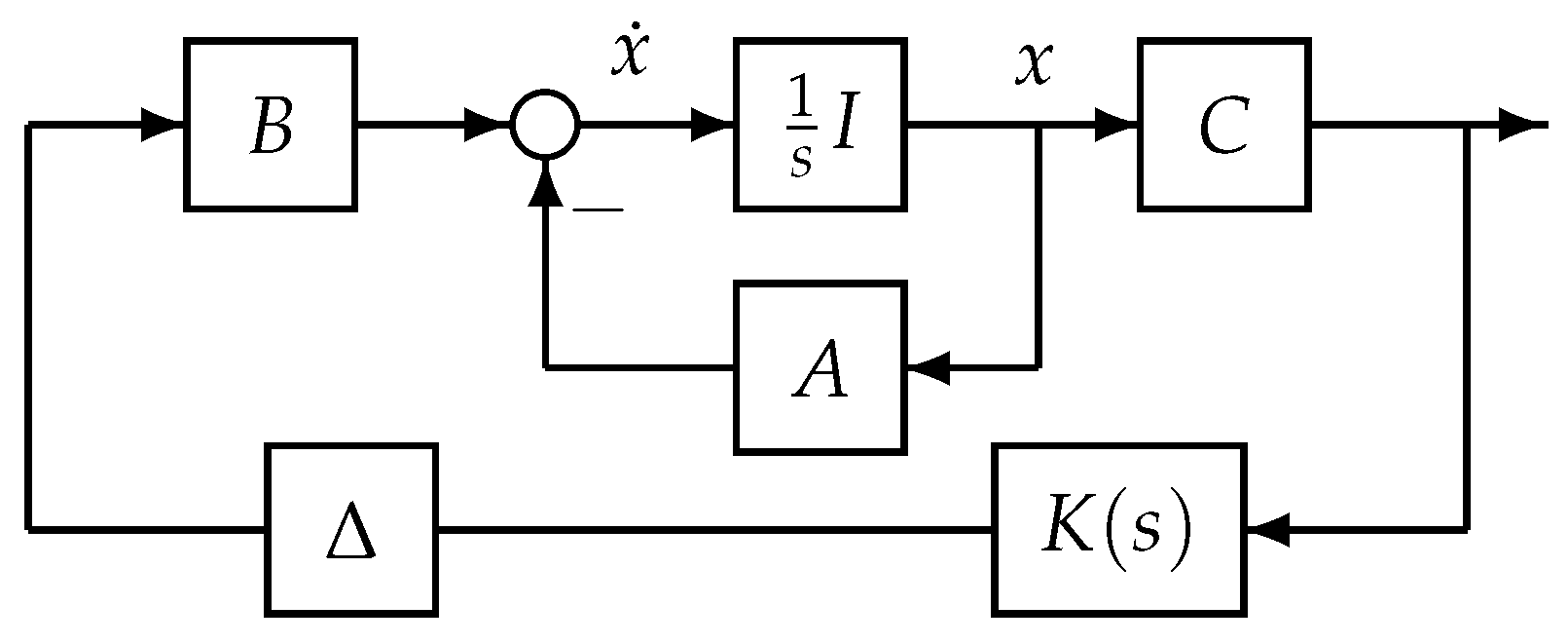
Figure 2.
Feedback control structure.
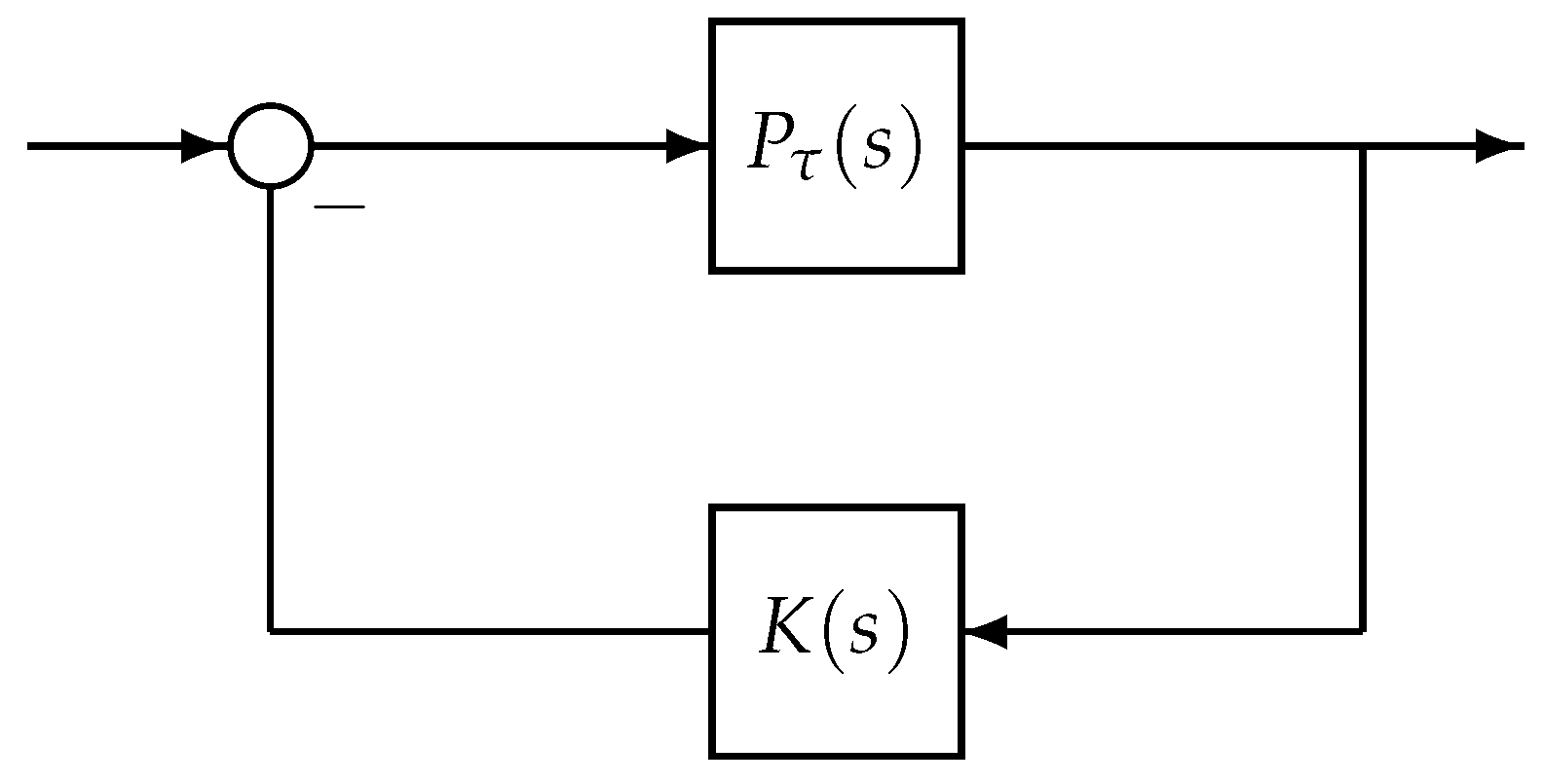
Figure 3.
Small gain setup of the feedback control system (1).
Figure 3.
Small gain setup of the feedback control system (1).
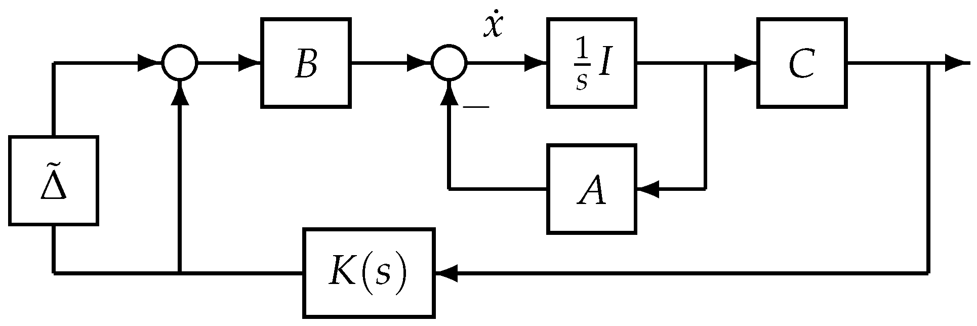
Figure 4.
Rational approximation for .

Figure 5.
Stabilizability region of system (50).
Figure 5.
Stabilizability region of system (50).

Figure 6.
System states of system (50) with controller K.
Figure 6.
System states of system (50) with controller K.

© 2017 by the author. Licensee MDPI, Basel, Switzerland. This article is an open access article distributed under the terms and conditions of the Creative Commons Attribution (CC BY) license (http://creativecommons.org/licenses/by/4.0/).
Share and Cite
MDPI and ACS Style
Zhu, J. On the Achievable Stabilization Delay Margin for Linear Plants with Time-Varying Delays. Mathematics 2017, 5, 55. https://doi.org/10.3390/math5040055
AMA Style
Zhu J. On the Achievable Stabilization Delay Margin for Linear Plants with Time-Varying Delays. Mathematics. 2017; 5(4):55. https://doi.org/10.3390/math5040055
Chicago/Turabian StyleZhu, Jing. 2017. "On the Achievable Stabilization Delay Margin for Linear Plants with Time-Varying Delays" Mathematics 5, no. 4: 55. https://doi.org/10.3390/math5040055
Note that from the first issue of 2016, this journal uses article numbers instead of page numbers. See further details here.