Invariant Solutions for a Class of Perturbed Nonlinear Wave Equations

Department of Mathematics and Statistics, King Fahd University of Petroleum and Minerals, Dhahran 31261, Saudi Arabia
*
Author to whom correspondence should be addressed.
Mathematics 2017, 5(4), 59; https://doi.org/10.3390/math5040059
Submission received: 22 September 2017
/
Revised: 20 October 2017
/
Accepted: 23 October 2017
/
Published: 1 November 2017
Abstract
:Approximate symmetries of a class of perturbed nonlinear wave equations are computed using two newly-developed methods. Invariant solutions associated with the approximate symmetries are constructed for both methods. Symmetries and solutions are compared through discussing the advantages and disadvantages of each method.
Mathematics Subject Classification:
35L05; 35L70; 58J70; 74J30; 76M601. Introduction
Approximate Lie symmetry is based on the utilization of the perturbation approach in finding symmetries of certain equations. Baikov, Gazizov and Ibragimov [1] proved an approximate Lie theorem enabling one to construct approximate symmetries of differential equations that are stable under small perturbations. Fushchich and Shtelen [2] and later Gazizov [3] introduced approximate symmetries of differential equations with small perturbations and showed that the these symmetries form an approximate Lie algebra. Since then, many authors have used the approximate Lie symmetries to study nonlinear partial differential equations (PDEs) with a small parameter; see, for instance, [4,5,6,7] and the references therein.
Pakdermirli, Yurusoy and Dolapci [8] provided a comparison between several methods that use approximate symmetries. Valenti [9] calculated the solution of a model describing dissipative media using the generator of the first-order approximate symmetries. Bokhari, Kara and Zaman [4] considered some nonlinear evolution equations with a small parameter and their symmetries. On the other hand, a refined invariant subspace method to determine subspaces of solutions to nonlinear wave equations was discussed in [10]. Zhi-Yong, Yu-Fu and Xue-Lin [11] performed classification and gave approximate solutions to a class of perturbed nonlinear wave equation employing the method originated from Fushchich and Shtelen. In [12], the authors introduced a new method to obtain the approximate symmetry of the nonlinear evolution equation from perturbations.
In this paper, we study the approximate symmetries of a class of perturbed nonlinear wave equations given by:
Lie group theory provides a systematic way of finding exact solutions of differential equations. If the problem involves a small parameter, then an approximate solution instead of an exact solution can be sought. We employ two methods in which a combination of Lie symmetries and perturbation theory is used to find approximate Lie symmetries and invariant solutions.
Method I was introduced by Baikov, Gazizov and Ibragimov [1,13]. In this method, an approximate generator is calculated to obtain the solution. The Lie operator is expanded in a perturbation series other than perturbation for dependent variables as in the usual case. In other words, it is assumed that the perturbed differential equation is of the form:
where is the unperturbed equation and is the perturbed term.
Theorem 1.
The exact symmetry of the unperturbed equation denoted by can be obtained using the equation Applying the auxiliary function:
we deduce the vector field from the relation:
After computing the approximate symmetries, the corresponding invariant solutions are constructed via the classical Lie symmetry method [14]. One may refer the reader for some cases of studying unperturbed and perturbed non-linear wave equations to Bokhari, Kara, Karim, Zaman [15] and Zhi-Yong, Yu-Fu and Xue-Lin [12]. Ahmed, Bokhari, Kara and Zaman [16] provided a classification of the symmetries of the unperturbed nonlinear dimensional wave equation with its respective commutator table.
Method II is due to Fushchich and Shtelen [2] and later followed by Euler et al. [17] and Euler and Euler [18]. In this method, the dependent variables are expanded in a perturbation series as is done in the usual perturbation analysis (see, e.g., [19,20]). The approximate symmetry of the original equation is defined to be the exact symmetry of the coupled equations.
Consider the general m-th order nonlinear evolution equation:
where , is a small parameter and E is a smooth function of the indicated variables. Expanding the dependent variable in the small parameter yields:
Inserting expansion Equation (5) into the original Equation (4) and separating at each order of the perturbed parameter, one has:
and hence, the exact symmetry of system Equation (6) is the approximate symmetry of the original Equation (4).
The outline of this paper is as follows. In Section 2, we construct invariant solutions of a perturbed nonlinear -dimensional wave equation. In Section 3, we consider Equation (1) with and obtain exact and approximate symmetries of the equation using the approximate Lie symmetry Method I. Moreover approximate invariant solutions of the perturbed non-linear wave equation based on the Lie group method are constructed. In Section 4, we discuss Equation (1) with and compute approximate symmetries of the equation with a forcing term using both the approximate Lie symmetry methods. We compare these different methods and discuss the advantages of using one over the other. Moreover, approximate invariant solutions of the nonlinear wave equation with a forcing term based on the Lie group method are constructed.
2. Perturbed Nonlinear (1 + 1)-Dimension Wave Equation
Consider the perturbed nonlinear wave equation (see e.g., [21]):
The approximate group generator of Equation (7) is of the form:
where are all unknown functions of and The infinitesimal generator for the unperturbed equation is a vector field in the three-dimensional space (two independent variables and one dependent variable):
The prolongation of the infinitesimal symmetry generator is given by:
The symmetry criterion of Equation (10) yields the relation:
Comparing coefficients of we obtain the following system of determining equations
Solving this system of PDEs, we obtain:
where are arbitrary constants. Thus,
To determine the auxiliary function we consider:
or:
where is the second prolongation of . This implies that:
Hence,
Substituting and into Equation (16) gives:
The determining equation for deformations is written as:
where denotes the second prolongation of the operator:
We obtain the following system of the determining equations for Equation (18):
Solving the above system yields:
Substituting Equations (12) and (20) into Equation (8), we obtain the following approximate symmetries for Equation (7):
In Table 1, we show that the generators span an eight-dimensional approximate Lie algebra and, hence, generate an eight-parameter approximate transformation group.
Approximate Invariant Solution
Using the symmetry we obtain:
The first equation in Equation (22) has two functionally independent solutions,
Substituting into the second equation in Equation (22) and taking its simplest solution we obtain one invariant in Equation (23),
Now, we substitute the solution of the first equation in Equation (22) into the second equation in Equation (22) and get a non-homogeneous linear equation:
The corresponding characteristic equation are:
for which the first integral We obtain:
Assuming we get the second invariant in Equation (23),
Note that invariants’ Equations (24) and (25) are functionally independent. Letting i.e.,
and solving for in the first order of precision,
The approximately invariant solution is given by:
From Equation (7), we obtain:
Setting we have and:
3. Perturbed Nonlinear (2 + 1)-Dimension Wave Equation
Consider the perturbed nonlinear wave equation:
where is a small parameter. Putting gives:
The first method is used to obtain a complete approximate symmetry classification of Equation (28) with the first order of precision The approximate group generator of Equation (28) is of the form:
where and are unknown functions of and
3.1. Exact Symmetries
To find the exact symmetries, we solve the determining equation:
where is the unperturbed part of Equation (28) and is the second prolongation of the infinitesimal generator given by:
Here, and denote the total derivative operators with respect to and respectively,
Equation (32) gives the following system of equations:
Solving this system of PDEs, one has:
where and are arbitrary constants. Hence, the infinitesimal generator for Equation (28) is:
3.2. Approximate Symmetries
The auxiliary function H is given by:
Now, we calculate operator by solving the inhomogeneous determining equation:
which can be written as:
Equation (39) generates the following system of equations:
Solving this system of PDEs, we obtain:
where and are arbitrary constants. Thus, the approximate symmetries of Equation (28) are:
Remark 1.
In Table 2, we show that the previous generators span a twelve-dimensional approximate Lie algebra and, hence, generate a twelve-parameter approximate transformations group.
3.3. Approximate Invariant Solutions
The approximate invariant for Equation (42) is of the form:
determined by the equation Using the notation:
where:
for operator Equation (42), we write the determining equation for the approximate invariants in the form:
or:
The first equation in Equation (43) has two functionally independent solutions:
Substituting into the second equation in Equation (43) and taking its simplest solution we obtain one invariant in Equation (44),
Note that the dependent variable u does not appear in Equation (45). Now, we substitute the solution of the first equation in Equation (43) into the second equation in Equation (43) and obtain non-homogeneous linear equation:
The corresponding characteristic equations are:
with the first integral Therefore, the second equation:
gives:
Assuming that we obtain the second invariant in Equation (44),
Note that and are functionally independent. Letting i.e.,
and solving for in the first order of precision,
yield the approximate invariant solution:
From Equation (28), we obtain:
Case I: Let be of the form From Equation (49), one obtains:
For we have:
An approximate solution for this case is depicted in Figure 1.
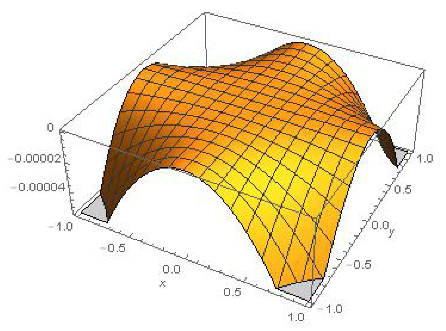
Let From Equations (51) and (52), we obtain:
and:
where are arbitrary constants. Therefore, a solution in this case is of the form:
We plot an approximate solution for this case in Figure 2.
4. Nonlinear Wave Equation with a Forcing Term
In this section, we discuss the nonlinear (2 + 1)-dimensional wave equation with a forcing term:
4.1. Approximate Symmetries by Method I
Exact symmetries of the unperturbed part () of Equation (56) are given by:
where and are arbitrary constants.
Consider the auxiliary function:
where:
Now we calculate the operator with the condition that
Condition Equation (60) can be written as:
where is the second prolongation of
Equation (61) yields the following system of equations:
Solving this system of PDEs, we obtain:
where and are arbitrary constants.
Case I: The scaling operator:
is not stable, and hence, Equation (56) does not inherit symmetries of its unperturbed part.
Case II: Solving the first order linear differential equation we obtain , where is a constant. The approximate symmetry generator of Equation (56) is given by:
These additional symmetries are actually the same as those obtained from the unperturbed equation that are considered as trivial symmetries. To summarize: in this case, Method I only gives trivial symmetries.
4.2. Approximate Symmetries by Method II
We expand the dependent variable to the first order of as follows:
Taylor expansion of f in the first order of precision is given by:
Substituting the above expansion into Equation (56) and separating at each order of perturbation parameter, one may obtain:
Now, the infinitesimal generator for the problem is:
Using standard Lie group analysis, we obtain the infinitesimals as follows:
where and are arbitrary constants. Hence, we have the following symmetries:
4.3. Approximate Invariant Solution
Using from Equation (67), we retrieve the following characteristic equations:
The equations in Equation (68) yield and suggest that Derivatives of dependent variables v and w with respect to x and y are:
These equations lead to the following second order ordinary differential equations:
We have where and are arbitrary constants of the integration. Thus, Put The second equation of Equation (69) is reduced to the following second-order ordinary differential equation:
Observe that it is not straight forward to obtain a solution for Equation (70). However, we may obtain an asymptotic estimate of the solution of Equation (70) using the asymptotic expansions [22].
Definition 1.
The function as if there exists a constant C such that
In Equation (70), we have and as For large values of Equation (70) is asymptotically equivalent to the following equation:
The solution of the above non-homogeneous Cauchy–Euler equation is:
where are constants. Lastly, we re-cast the solution in original coordinates as:
5. Concluding Remarks
In this work, we have studied a class of perturbed nonlinear wave equations via Lie symmetry analysis. Two methods have been employed to obtain approximate symmetries used to construct invariant solutions of the equations. There was a case where Method I gives only trivial solutions. We applied Method II to this case and obtained the invariant solutions of the equation. Many problems arising from physical or engineering situations may be dealt with by approximate Lie symmetry analysis. We plan to investigate modified and perturbed forms of Korteweg-de Vries (KdV) equations using this approach.
Acknowledgments
The authors are grateful to King Fahd University of Petroleum & Minerals for supporting the research.
Author Contributions
Waheed: working out symmetries and approximation. Zaman: proposing, guiding and leading. Saleh: working out plan, verifying, writing up and final form.
Conflicts of Interest
The authors declare no conflict of interest.
References
- Baikov, V.A.; Gazizov, R.K.; Ibragimov, N. Approximate symmetries. Mat. Sb. 1988, 178, 435–450. [Google Scholar] [CrossRef]
- Fushchich, W.; Shtelen, W. On approximate symmetry and approximate solutions of the nonlinear wave equation with a small parameter. J. Phys. A Math. Gen. 1989, 22, L887. [Google Scholar] [CrossRef]
- Gazizov, R.K. Lie algebras of approximate symmetries. J. Nonlinear Math. Phys. 1996, 3, 96–101. [Google Scholar] [CrossRef]
- Bokhari, A.H.; Kara, A.; Zaman, F.D. Invariant solutions of certain nonlinear evolution type equations with small parameters. Appl. Math. Comput. 2006, 182, 1075–1082. [Google Scholar] [CrossRef]
- Jefferson, G.; Carminati, J. Asp: Automated symbolic computation of approximate symmetries of differential equations. Comput. Phys. Commun. 2013, 184, 1045–1063. [Google Scholar] [CrossRef]
- Li, X.; Qian, S. Approximate symmetry reduction to the perturbed coupled kdv equations derived from two-layer fluids. Math. Sci. 2012, 6, 13. [Google Scholar] [CrossRef]
- Zhang, Z.Y.; Chen, Y.F.; Yong, X.L. Classification and approximate solutions to a class of perturbed nonlinear wave equations. Commun. Theor. Phys. 2009, 52, 769–772. [Google Scholar]
- Pakdemirli, M.; Yürüsoy, M.; Dolapci, I. Comparison of approximate symmetry methods for differential equations. Acta Appl. Math. 2004, 80, 243–271. [Google Scholar] [CrossRef]
- Valenti, A. Approximate symmetries for a model describing dissipative media. In Proceedings of the 10th International Conference in Modern Group Analysis, Larnaca, Cyprus, 24–31 October 2004; Volume 236, p. 243. [Google Scholar]
- Ma, W.X. A refined invariant subspace method and applications to evolution equations. Sci. China Math. 2012, 55, 1769–1778. [Google Scholar] [CrossRef]
- Zhang, Z.; Gao, B.; Chen, Y. Second-order approximate symmetry classification and optimal system of a class of perturbed nonlinear wave equations. Commun. Nonlinear Sci. Numer. Simul. 2011, 16, 2709–2719. [Google Scholar] [CrossRef]
- Zhang, Z.-Y.; Yong, X.-L.; Chen, Y.-F. A new method to obtain approximate symmetry of nonlinear evolution equation from perturbations. Chin. Phys. B 2009, 18, 2629–2633. [Google Scholar]
- Baikov, V.; Gazizov, R.; Ibragimov, N. Approximate transformation groups and deformations of symmetry lie algebras. In CRC Handbook of Lie Group Analysis of Differential Equations; CRC Press: Boca Raton, FL, USA, 1996; Volume 3. [Google Scholar]
- Grigotieve, Y.N.; Ibragimov, N.H.; Kovalev, V.F.; Meleshko, S.V. Symmetries of Integro-Differential Equations with Application in Mechanics and Plasma Physics; Springer: Berlin, Germany, 2010. [Google Scholar]
- Bokhari, A.H.; Kara, A.; Karim, M.; Zaman, F.D. Invariance analysis and variational conservation laws for the wave equation on some manifolds. Int. J. Theor. Phys. 2009, 48, 1919–1928. [Google Scholar] [CrossRef]
- Ahmad, A.; Bokhari, A.H.; Kara, A.; Zaman, F.D. A complete symmetry classification and reduction of some classes of the nonlinear (1-2) wave equation. Quaest. Math. 2010, 33, 75–94. [Google Scholar] [CrossRef]
- Euler, M.; Euler, N.; Kohler, A. On the construction of approximate solutions for a multidimensional nonlinear heat equation. J. Phys. A Math. Gen. 1994, 27, 2083–2092. [Google Scholar] [CrossRef]
- Euler, N.; Euler, M. Symmetry properties of the approximations of multidimensional generalized van der pol equations. J. Nonlinear Math. Phys. 1994, 1, 41–59. [Google Scholar] [CrossRef]
- Ma, W.X.; Fuchssteiner, B. Integrable theory of the perturbation equations. Chaos Soliton Fractal 1996, 7, 1227–1250. [Google Scholar] [CrossRef]
- Ma, W.X. A bi-Hamiltonian formulation for triangular systems by perturbations. J. Math. Phys. 2002, 43, 1408–1421. [Google Scholar] [CrossRef]
- Ibragimov, N.H.; Kovalev, V.F. Approximate and Renormgroup Symmetries; Springer: Berlin, Germany, 2009. [Google Scholar]
- Murray, J.D. Asymptotic analysi. In Applied Mathematical Sciences; Springer: New York, NY, USA, 1984; Volume 1. [Google Scholar]
Figure 1.
CaseI: approximate invariant solution of Equation (28) for
Figure 1.
CaseI: approximate invariant solution of Equation (28) for
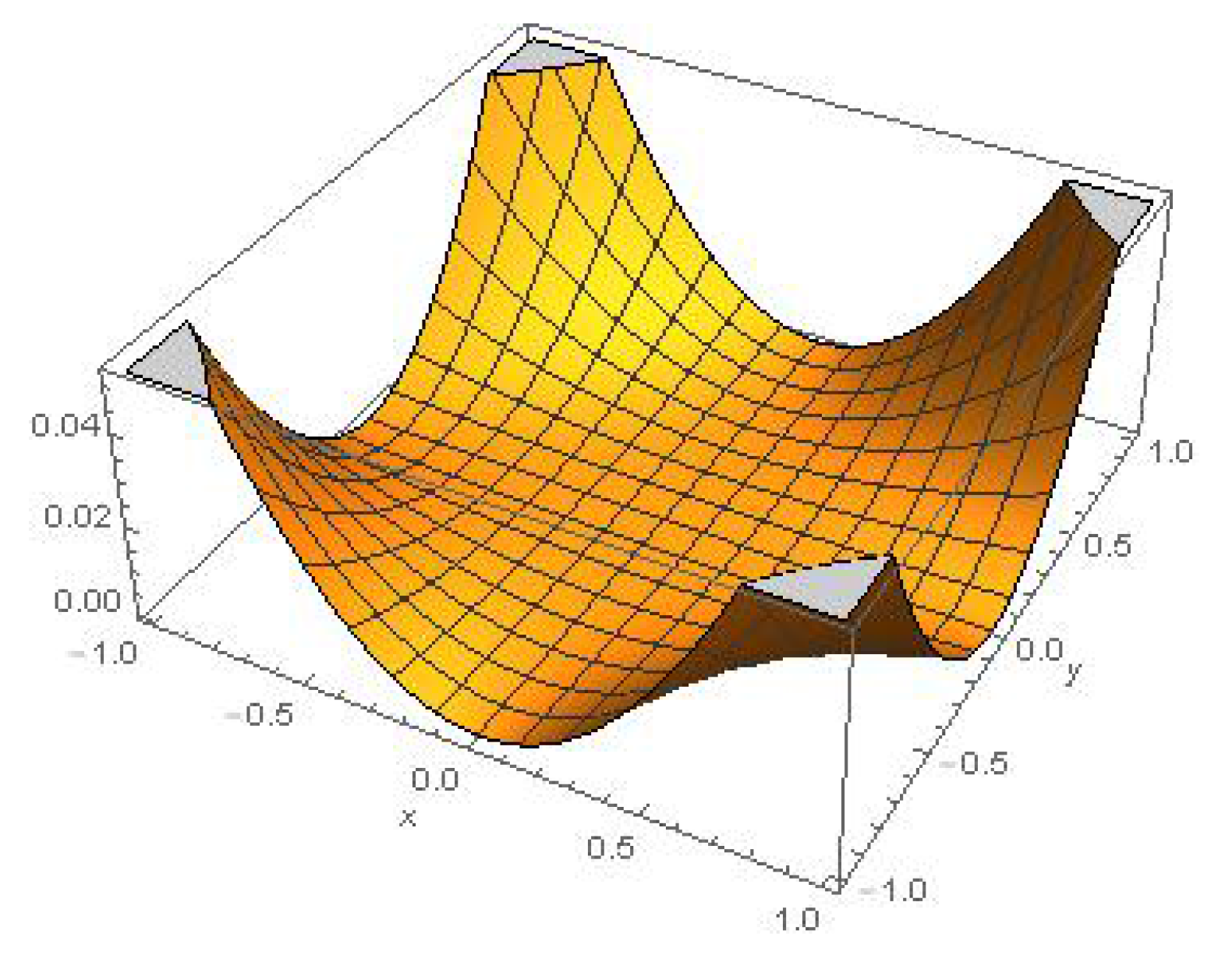
Figure 2.
Case II:approximate invariant solution of Equation (28) for
Figure 2.
Case II:approximate invariant solution of Equation (28) for

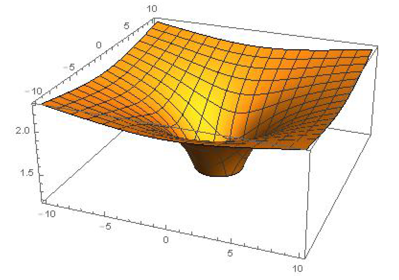
Figure 3.
Invariant solution of the unperturbed equation of Equation (56) for , .
Figure 3.
Invariant solution of the unperturbed equation of Equation (56) for , .

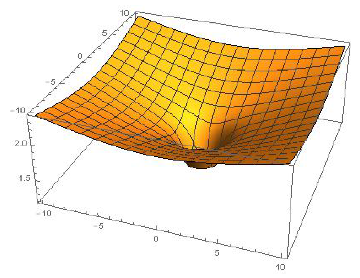
Figure 4.
Approximate invariant solution of Equation (56) for .
Figure 4.
Approximate invariant solution of Equation (56) for .


Table 1.
Approximate commutators of approximate symmetry of the perturbed non-linear wave equation.
| 0 | 0 | 0 | 0 | 0 | 0 | |||
| 0 | 0 | 0 | 0 | |||||
| 0 | 0 | 0 | 0 | 0 | 0 | |||
| 0 | 0 | 0 | 0 | 0 | 0 | 0 | ||
| 0 | 0 | 0 | 0 | 0 | 0 | |||
| 0 | 0 | 0 | 0 | 0 | 0 | 0 | ||
| 0 | 0 | 0 | 0 | 0 | 0 | 0 | ||
| 0 | 0 | 0 | 0 | 0 | 0 |
Table 2.
Approximate commutator table of approximate symmetries of the perturbed non-linear wave equation.
Table 2.
Approximate commutator table of approximate symmetries of the perturbed non-linear wave equation.
| 0 | 0 | 0 | 0 | 0 | 0 | 0 | 0 | 0 | ||||
| 0 | 0 | 0 | 0 | 0 | 0 | 0 | 0 | |||||
| 0 | 0 | 0 | 0 | 0 | 0 | 0 | 0 | |||||
| 0 | 0 | 0 | 0 | 0 | 0 | 0 | 0 | 0 | 0 | |||
| 0 | 0 | 0 | 0 | 0 | 0 | 0 | 0 | 0 | 0 | |||
| 0 | 0 | 0 | 0 | 0 | 0 | 0 | 0 | |||||
| 0 | 0 | 0 | 0 | 0 | 0 | 0 | 0 | 0 | 0 | |||
| 0 | 0 | 0 | 0 | 0 | 0 | 0 | 0 | 0 | 0 | |||
| 0 | 0 | 0 | 0 | 0 | 0 | 0 | 0 | 0 | 0 | |||
| 0 | 0 | 0 | 0 | 0 | 0 | 0 | 0 | 0 | 0 | 0 | ||
| 0 | 0 | 0 | 0 | 0 | 0 | 0 | 0 | 0 | 0 | 0 | ||
| 0 | 0 | 0 | 0 | 0 | 0 | 0 | 0 | 0 | 0 | 0 |
Table 3.
Commutators span six-dimensional Lie algebra.
| 0 | 0 | 0 | 0 | |||
| 0 | 0 | 0 | 0 | |||
| 0 | 0 | 0 | 0 | |||
| 0 | 0 | 0 | 0 | 0 | ||
| 0 | 0 | 0 | 0 | 0 | ||
| 0 | 0 | 0 | 0 |
© 2017 by the authors. Licensee MDPI, Basel, Switzerland. This article is an open access article distributed under the terms and conditions of the Creative Commons Attribution (CC BY) license (http://creativecommons.org/licenses/by/4.0/).
Share and Cite
MDPI and ACS Style
Ahmed, W.A.; Zaman, F.D.; Saleh, K. Invariant Solutions for a Class of Perturbed Nonlinear Wave Equations. Mathematics 2017, 5, 59. https://doi.org/10.3390/math5040059
AMA Style
Ahmed WA, Zaman FD, Saleh K. Invariant Solutions for a Class of Perturbed Nonlinear Wave Equations. Mathematics. 2017; 5(4):59. https://doi.org/10.3390/math5040059
Chicago/Turabian StyleAhmed, Waheed A., F. D. Zaman, and Khairul Saleh. 2017. "Invariant Solutions for a Class of Perturbed Nonlinear Wave Equations" Mathematics 5, no. 4: 59. https://doi.org/10.3390/math5040059
Note that from the first issue of 2016, this journal uses article numbers instead of page numbers. See further details here.