Graph Structures in Bipolar Neutrosophic Environment


1
Department of Mathematics, University of the Punjab, New Campus, Lahore 54590, Pakistan
2
Mathematics & Science Department, University of New Mexico, 705 Gurley Ave., Gallup, NM 87301, USA
*
Author to whom correspondence should be addressed.
Mathematics 2017, 5(4), 60; https://doi.org/10.3390/math5040060
Submission received: 14 September 2017
/
Revised: 18 October 2017
/
Accepted: 27 October 2017
/
Published: 6 November 2017
Abstract
:A bipolar single-valued neutrosophic (BSVN) graph structure is a generalization of a bipolar fuzzy graph. In this research paper, we present certain concepts of BSVN graph structures. We describe some operations on BSVN graph structures and elaborate on these with examples. Moreover, we investigate some related properties of these operations.
MSC:
03E72; 05C72; 05C78; 05C991. Introduction
Fuzzy graphs are mathematical models for dealing with combinatorial problems in different domains, including operations research, optimization, computer science and engineering. In 1965, Zadeh [1] proposed fuzzy set theory to deal with uncertainty in abundant meticulous real-life phenomena. Fuzzy set theory is affluently applicable in real-time systems consisting of information with different levels of precision. Subsequently, Atanassov [2] introduced the idea of intuitionistic fuzzy sets in 1986. However, for many real-life phenomena, it is necessary to deal with the implicit counter property of a particular event. Zhang [3] initiated the concept of bipolar fuzzy sets in 1994. Evidently bipolar fuzzy sets and intuitionistic fuzzy sets seem to be similar, but they are completely different sets. Bipolar fuzzy sets have large number of applications in image processing and spatial reasoning. Bipolar fuzzy sets are more practical, advantageous and applicable in real-life phenomena. However, both bipolar fuzzy sets and intuitionistic fuzzy sets cope with incomplete information, because they do not consider indeterminate or inconsistent information that clearly appears in many systems of different fields, including belief systems and decision-support systems. Smarandache [4] introduced neutrosophic sets as a generalization of fuzzy sets and intuitionistic fuzzy sets. A neutrosophic set has three constituents: truth membership, indeterminacy membership and falsity membership, for which each membership value is a real standard or non-standard subset of the unit interval . In real-life problems, neutrosophic sets can be applied more appropriately by using the single-valued neutrosophic sets defined by Smarandache [4] and Wang et al. [5]. Deli et al. [6] considered bipolar neutrosophic sets as a generalization of bipolar fuzzy sets. They also studied some operations and applications in decision-making problems.
On the basis of Zadeh’s fuzzy relations [7], Kauffman defined fuzzy graphs [8]. In 1975, Rosenfeld [9] discussed a fuzzy analogue of different graph-theoretic ideas. Later on, Bhattacharya [10] gave some remarks on fuzzy graphs in 1987. Akram [11] first introduced the notion of bipolar fuzzy graphs. In 2011, Dinesh and Ramakrishnan [12] studied fuzzy graph structures and discussed their properties. In 2016, Akram and Akmal [13] proposed the concept of bipolar fuzzy graph structures. Certain concepts on graphs have been discussed in [14,15,16,17,18,19]. Ye [20,21,22] considered several applications of single-valued neutrosophic sets. Inthis research paper, we present certain concepts of bipolar single-valued neutrosophic graph structures (BSVNGSs). We introduce some operations on BSVNGSs and elaborate on these with examples. Moreover, we investigate some relevant and remarkable properties of these operators.
2. Bipolar Single-Valued Neutrosophic Graph Structures
Definition 1.
[4] A neutrosophic set N on a non-empty set V is an object of the form
where and there is no restriction on the sum of , and for all .
Definition 2.
[5] A single-valued neutrosophic set N on a non-empty set V is an object of the form
where and the sum of , and is confined between 0 and 3 for all .
Definition 3.
[23] A BSVN set on a non-empty set V is an object of the form
where and . The positive values and denote the truth, indeterminacy and falsity membership values of an element , whereas negative values and indicate the implicit counter property of truth, indeterminacy and falsity membership values of an element .
Definition 4.
[23] A BSVN graph on a non-empty set V is a pair , where B is a BSVN set on V and R is a BSVN relation in V such that
We now define the BSVNGS.
Definition 5.
[30] A BSVNGS of a graph structure = is denoted by = , where is a BSVN set on the set V and are the BSVN sets on such that
for all Note that , for all , and represents an edge between two vertices b and d. In this paper we use in place of .
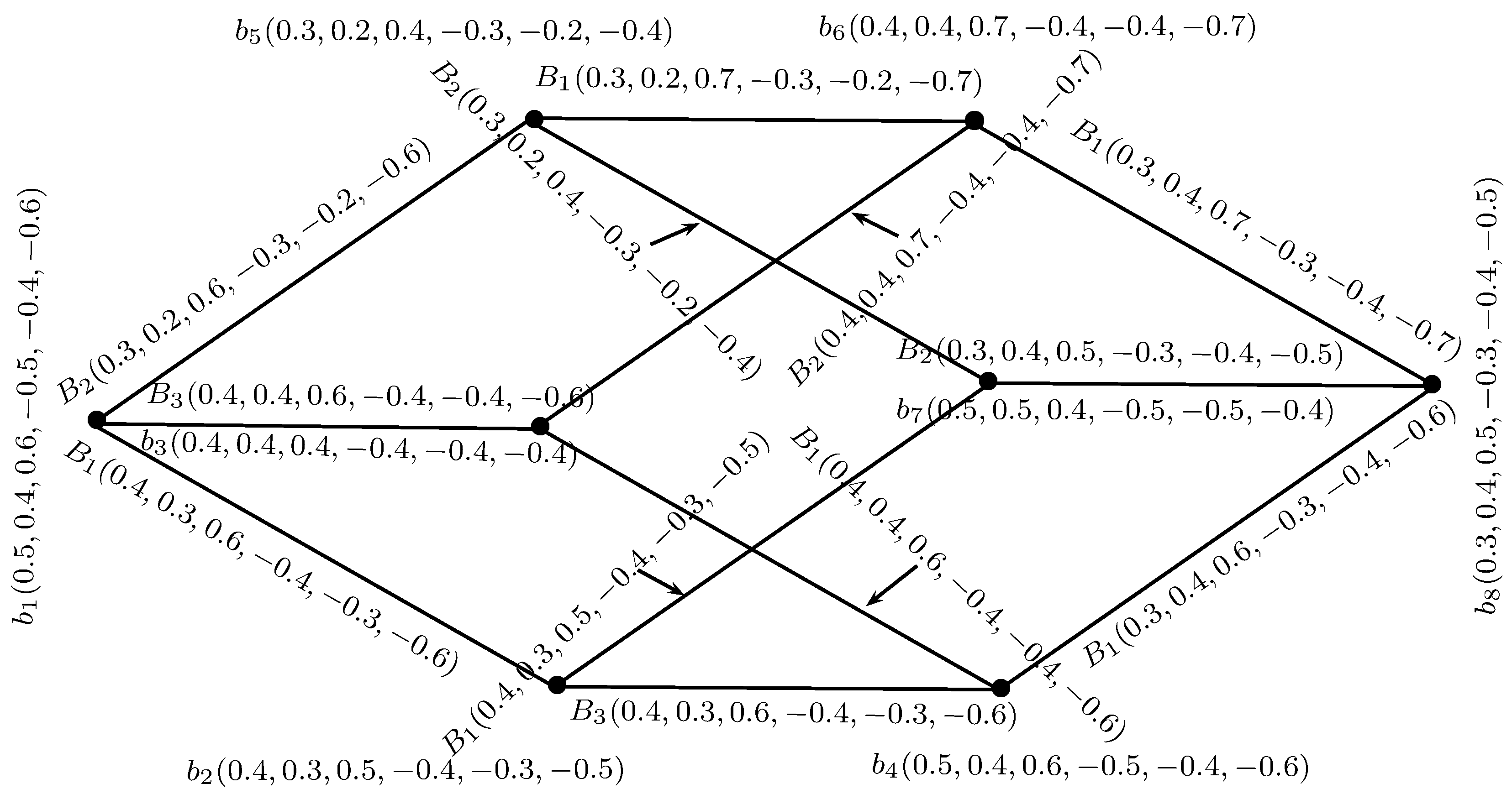
Example 1.
Consider a graph structure such that , , , and . Let B be a BSVN set on V given in Table 1 and , and be BSVN sets on , and , respectively, given in Table 2.
By direct calculations, it is easy to show that = is a BSVNGS. This BSVNGS is shown in Figure 1. Generated with LaTeXDraw 2.0.8 on Saturday March 11 20:30:24 PKT 2017.
Definition 6.
A BSVNGS = is called a -cycle if , is a -cycle.
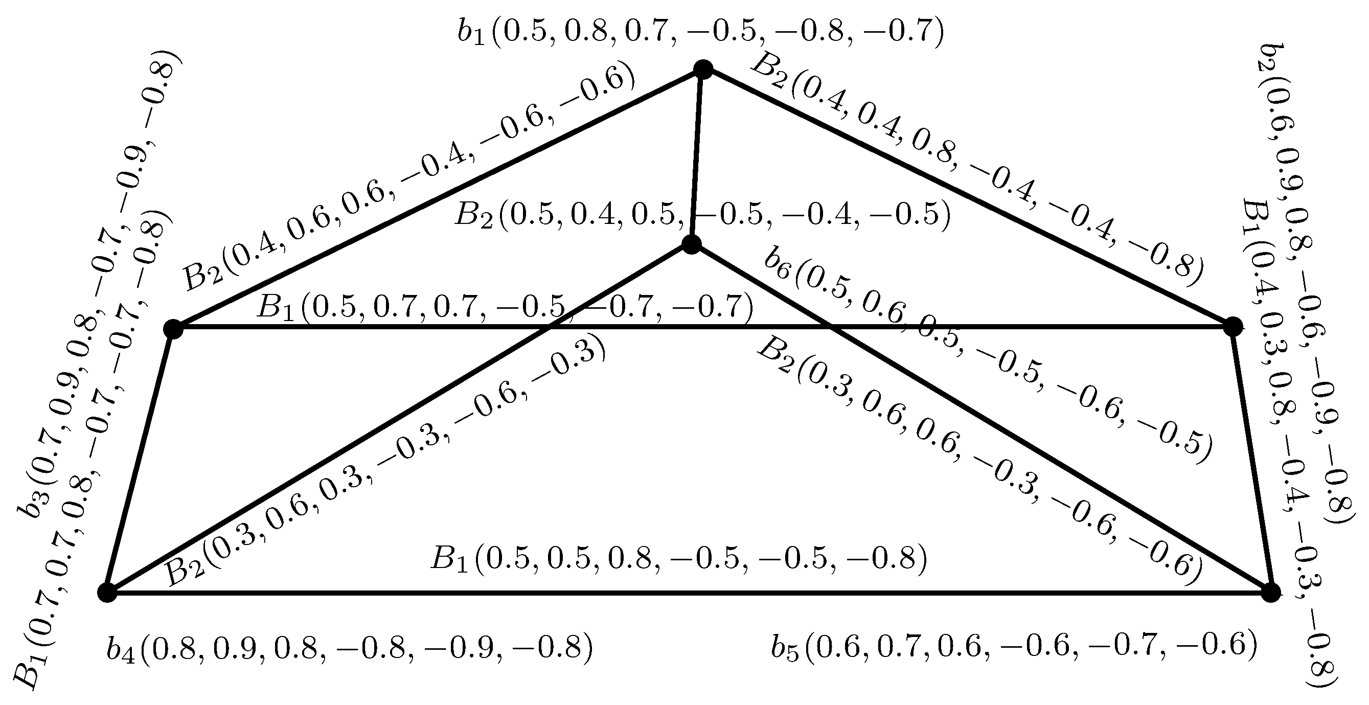
Example 2.
Consider a BSVNGS = as shown in Figure 2.
is a -cycle, as , is a -cycle, that is, ----.
Definition 7.
A BSVNGS = is a BSVN fuzzy -cycle (for any k) if is a -cycle and no unique -edge exists in , such that , , , , or
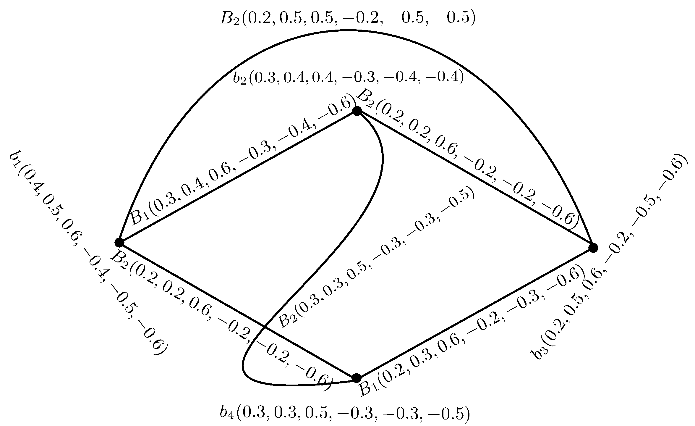
Example 3.
Consider a BSVNGS = as depicted in Figure 3.
, , , , or
Definition 8.
A sequence of vertices (distinct) in a BSVNGS = is called a -path, that is, , such that is a BSVN -edge, for all .
Example 4.
Consider a BSVNGS = as represented in Figure 4.
In this BSVNGS, the sequence of distinct vertices is a BSVN -path.
Definition 9.
Let = be a BSVNGS. The positive truth strength , positive falsity strength , and positive indeterminacy strength of a -path, = , are defined as
Similarly, the negative truth strength , negative falsity strength , and negative indeterminacy strength of a -path are defined as
Example 5.
Consider a BSVNGS = as shown in Figure 5.
In this BSVNGS, there is a -path, that is, = ,. Thus, = , = , = , = , = and = .
Definition 10.
Let = be a BSVNGS. Then
- The -positive strength of connectedness of truth between two nodes b and d is defined by = , such that = for and = = .
- The -positive strength of connectedness of indeterminacy between two nodes b and d is defined by = , such that = for and = = .
- The -positive strength of connectedness of falsity between two nodes b and d is defined by = , such that = for and = = .
- The -negative strength of connectedness of truth between two nodes b and d is defined by = , such that = for and = = .
- The -negative strength of connectedness of indeterminacy between two nodes b and d is defined by = , such that = for and = = .
- The -negative strength of connectedness of falsity between two nodes b and d is defined by = , such that = for and = = .
Definition 11.
Let = be a BSVNGS and “b” be a node in . Let be a BSVN subgraph structure of induced by such that
Then b is a BSVN fuzzy cut-vertex if , , , , and , for some . Note that vertex b is a BSVN fuzzy cut-vertex if , it is a BSVN fuzzy cut-vertex if , and it is a BSVN fuzzy cut-vertex if . Moreover, vertex b is a BSVN fuzzy cut-vertex if , it is a BSVN fuzzy cut-vertex if and it is a BSVN fuzzy cut-vertex if .
Example 6.
Consider a BSVNGS = as depicted in Figure 6, and let = be a BSVN subgraph structure of the BSVNGS , which is obtained through deletion of vertex .
The vertex is a BSVN fuzzy cut-vertex and a BSVN fuzzy cut-vertex, because , , , , , . , and .
Definition 12.
Suppose = is a BSVNGS and is a -edge. Let be a BSVN fuzzy spanning subgraph structure of , such that
Then is a BSVN fuzzy -bridge if , , , , and , for some . Note that is a BSVN fuzzy bridge if , it is a BSVN fuzzy bridge if and it is a BSVN fuzzy bridge if . Moreover, is a BSVN fuzzy bridge if , it is a BSVN fuzzy bridge if and it is a BSVN fuzzy bridge if .
Example 7.
Consider a BSVNGS = as depicted in Figure 6 and = , a BSVN spanning subgraph structure of the BSVNGS obtained by deleting-edge and that is shown in Figure 7.
This edge is a BSVN fuzzy -bridge, as = , = 0.4, = , = , = , , = = , = = , and = =
Definition 13.
A BSVNGS = is a -tree if is a -tree. Alternatively, is a -tree if has a subgraph induced by that forms a tree.
Example 8.
Consider the BSVNGS = as depicted in Figure 8.
This BSVNGS = is a -tree, as is a -tree.
Definition 14.
A BSVNGS = is a BSVN fuzzy -tree if has a BSVN fuzzy spanning subgraph structure = such that for all -edges, not in :
- is a -tree.
- , , , , , and .
In particular, is a BSVN fuzzy tree if , it is a BSVN fuzzy tree if , and it is a BSVN fuzzy tree if . Moreover, is a BSVN fuzzy tree if , it is a BSVN fuzzy tree if , and it is a BSVN fuzzy tree if .
Example 9.
Consider the BSVNGS = as depicted in Figure 9.
It is -tree, rather than a -tree. However, it is a BSVN fuzzy -tree, because it has a BSVN fuzzy spanning subgraph as a -tree, which is obtained through the deletion of the -edge from . Moreover, , , , , , , and
Now we define the operations on BSVNGSs.
Definition 15.
Let = and = be two BSVNGSs. The Cartesian product of and , denoted by
is defined as
- (i)
- (ii)
- for all ,
- (iii)
- (iv)
- for all ,
- (v)
- (vi)
- for all , .
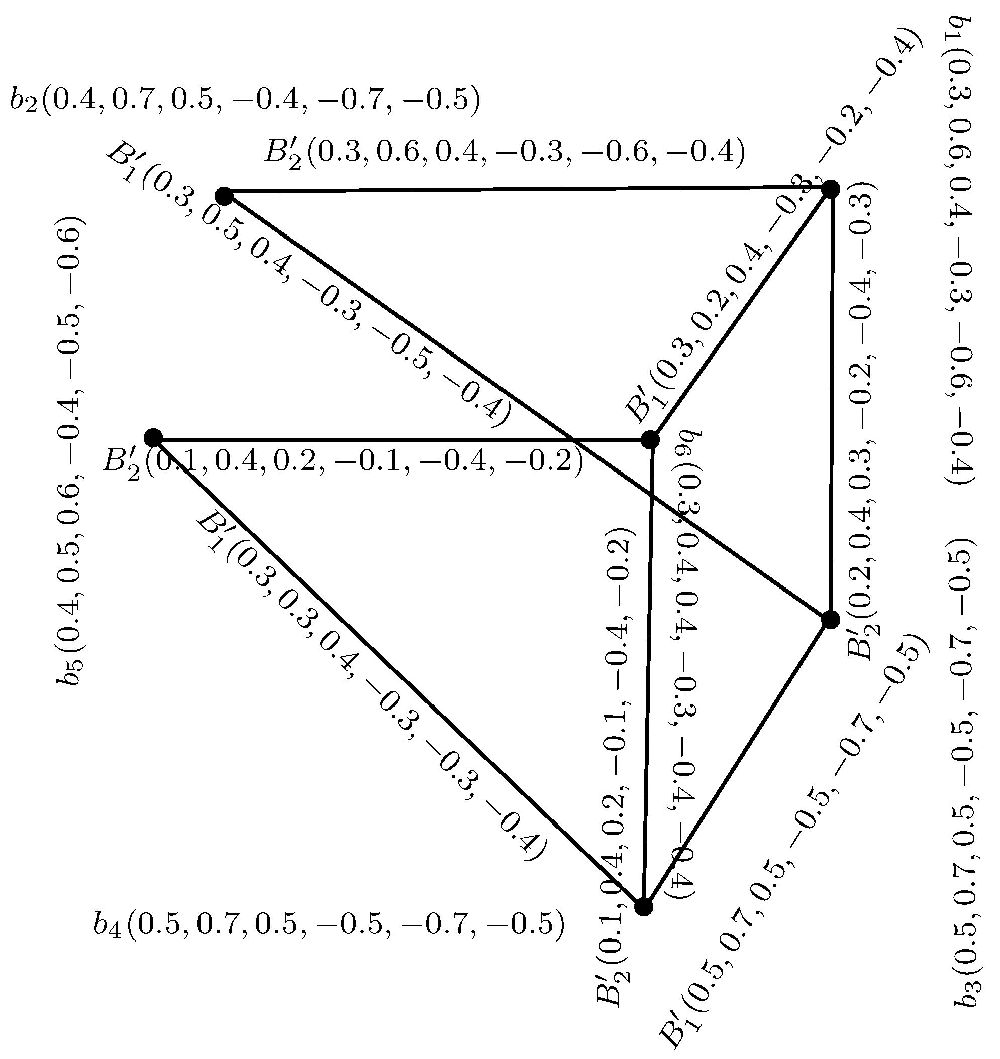
Example 10.
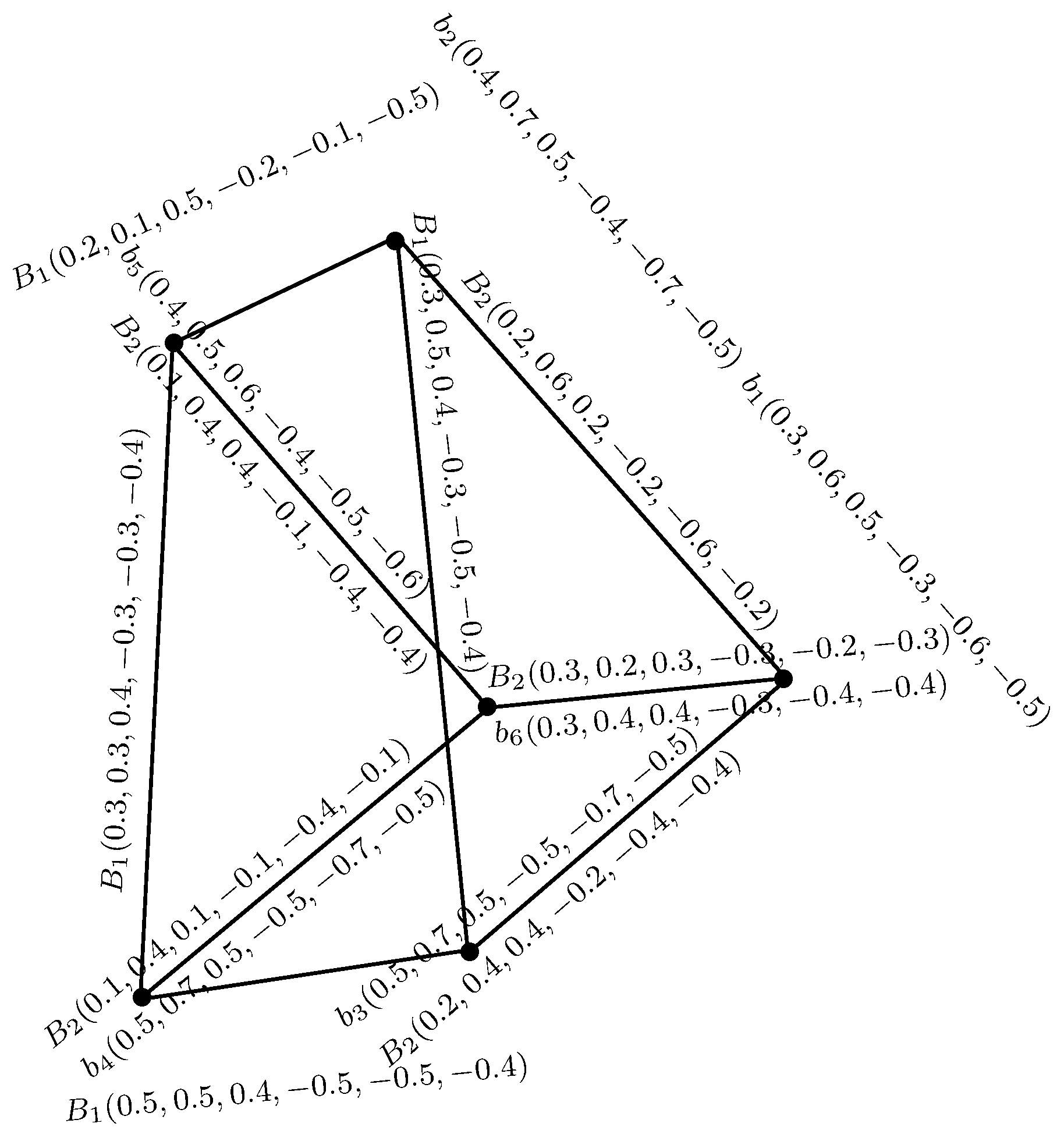
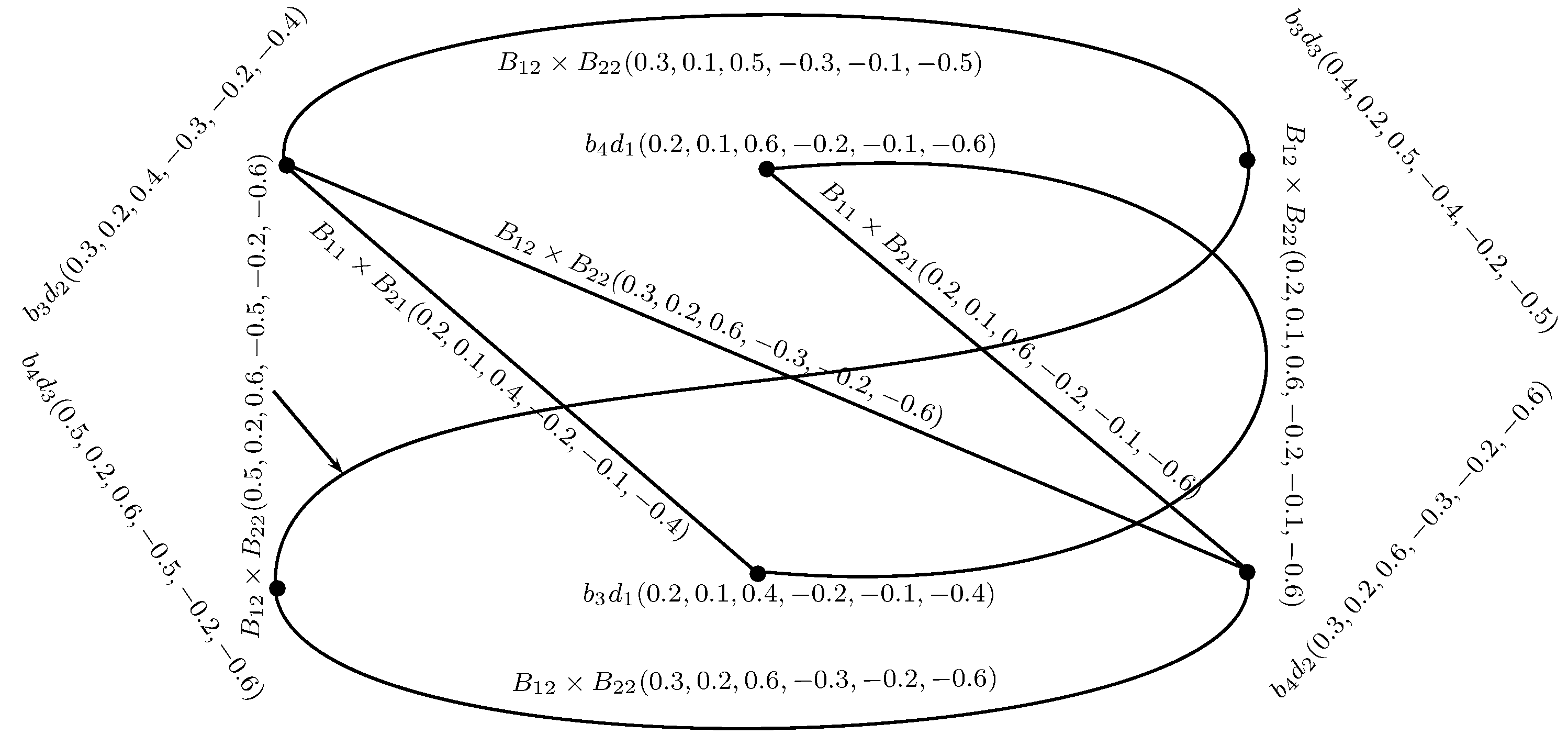
Consider = and = as BSVNGSs of GSs = and = , respectively, as depicted in Figure 10, where , , , and .
Theorem 1.
The Cartesian product = of two BSVNSGSs of GSs and is a BSVNGS of .
Proof.
Consider two cases:
- Case 1.
- For , ,for
- Case 2.
- For , ,for
Both cases hold for all . This completes the proof. ☐
Definition 16.
Let = and = be two BSVNGSs. The cross product of and , denoted by
is defined as
- (i)
- (ii)
- for all , and
- (iii)
- (iv)
- for all ,
Example 11.
Theorem 2.
The cross product = of two BSVNSGSs of GSs and is a BSVNGS of .
Proof.
For , ,
where and . ☐
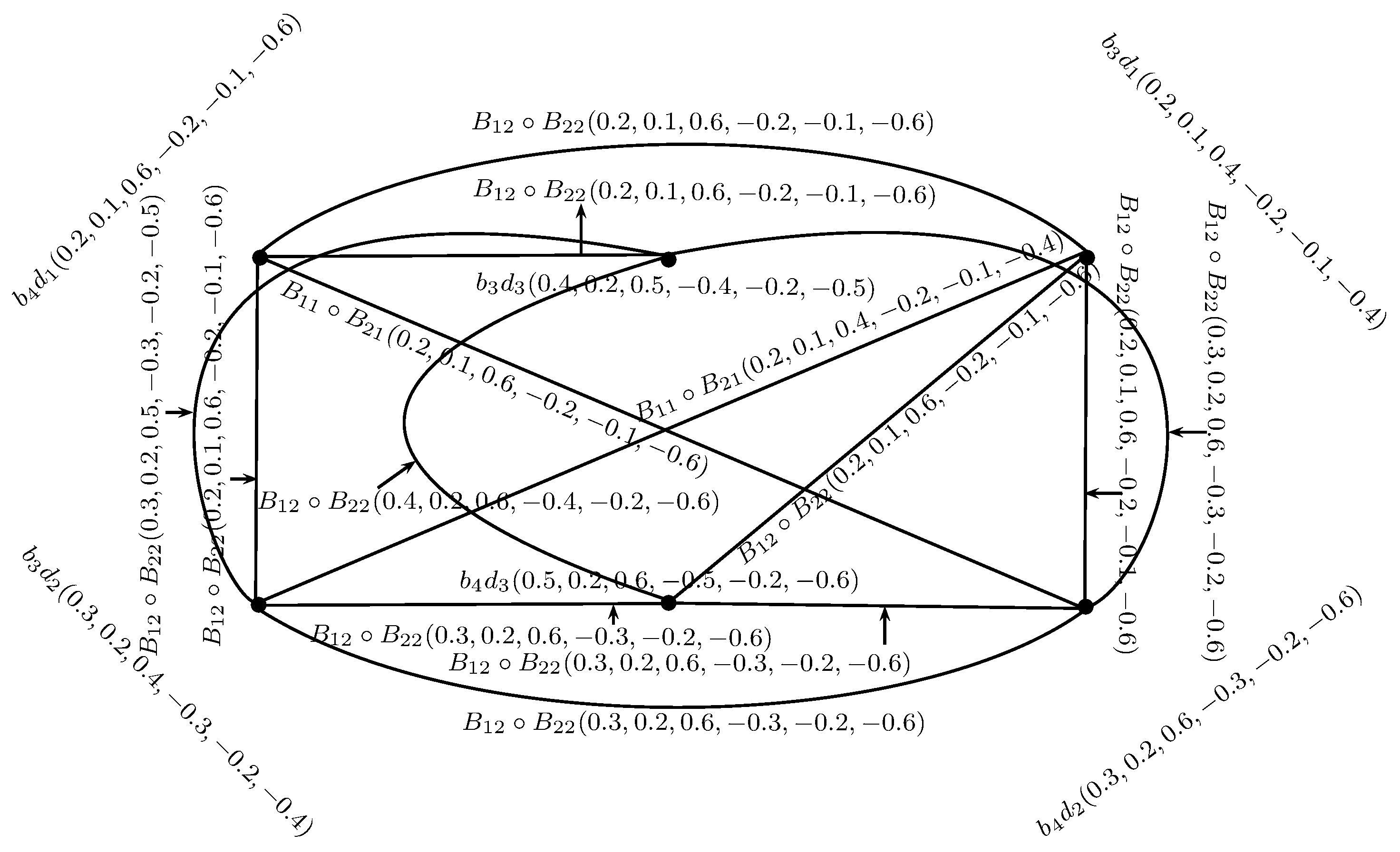
Definition 17.
Let = and = be two BSVNGSs. The composition of and , denoted by
is defined as
- (i)
- (ii)
- for all ,
- (iii)
- (iv)
- for all ,
- (v)
- (vi)
- for all , and
- (vii)
- (viii)
- for all , such that .
Example 12.
Theorem 3.
The composition = of two BSVNGSs of GSs and is a BSVNGS of .
Proof.
Consider three cases:
- Case 1.
- For , ,for
- Case 2.
- For , ,for
- Case 3.
- For , such that ,where .
All cases are satisfied for all . ☐
3. Conclusions
The notion of bipolar fuzzy graphs is applicable in several domains of engineering, expert systems, pattern recognition, signal processing, neural networks, medical diagnosis and decision-making. BSVNGSs show more flexibility, compatibility and precision for a system than single-valued neutrosophic graph structures. In this research paper, we introduced certain concepts of BSVNGSs and elaborated on them with suitable examples. Further, we defined some operations on BSVNGSs and investigated some relevant properties of these operations. We intend to generalize our research of fuzzification to (1) concepts of BSVN soft graph structures, (2) concepts of BSVN rough fuzzy graph structures, (3) concepts of BSVN fuzzy soft graph structures, and (4) concepts of BSVN rough fuzzy soft graph structures.
Acknowledgments
The authors are thankful to referees for their valuable comments and suggestion.
Author Contributions
Muhammad Akram, Muzzamal Sitara and Florentin Smarandache conceived and designed the experiments; Muhammad Akram performed the experiments; Muhammad Akram and Muzzamal Sitara analyzed the data; Florentin Smarandache contributed reagents/materials/analysis tools; Muzzamal Sitara wrote the paper.
Conflicts of Interest
The authors declare no conflict of interest regarding the publication of this research paper.
References
- Zadeh, L.A. Fuzzy sets. Inf. Control 1965, 8, 338–353. [Google Scholar] [CrossRef]
- Atanassov, K. Intuitionistic fuzzy sets. Fuzzy Sets Syst. 1986, 20, 87–96. [Google Scholar] [CrossRef]
- Zhang, W.-R. Bipolar fuzzy sets and relations: A computational framework for cognitive modeling and multiagent decision analysis. In Proceedings of the Industrial Fuzzy Control and Intelligent Systems Conference, and the NASA Joint Technology Workshop on Neural Networks and Fuzzy Logic Fuzzy Information Processing Society Biannual Conference, San Antonio, TX, USA, 18–21 December 1994; pp. 305–309. [Google Scholar]
- Smarandache, F. Neutrosophy Neutrosophic Probability, Set, and Logic; Amer Res Press: Rehoboth, MA, USA, 1998. [Google Scholar]
- Wang, H.; Smarandache, F.; Zhang, Y.Q.; Sunderraman, R. Single valued neutrosophic sets. Multispace Multistruct. 2010, 4, 410–413. [Google Scholar]
- Deli, I.; Ali, M.; Smarandache, F. Bipolar neutrosophic sets and their application based on multi-criteria decision making problems. In Proceedings of the International Conference IEEE Advanced Mechatronic Systems (ICAMechS), Beijing, China, 22–24 August 2015; pp. 249–254. [Google Scholar]
- Zadeh, L.A. Similarity relations and fuzzy orderings. Inf. Sci. 1971, 3, 177–200. [Google Scholar] [CrossRef]
- Kauffman, A. Introduction to the Theory of Fuzzy Subsets; Academic Press: Cambridge, MA, USA, 1973; Volume 1. [Google Scholar]
- Rosenfeld, A. Fuzzy graphs. In Fuzzy Sets and Their Applications; Zadeh, L.A., Fu, K.S., Eds.; Academic Press: New York, NY, USA, 1975; pp. 77–95. [Google Scholar]
- Bhattacharya, P. Some remarks on fuzzy graphs. Pattern Recognit. Lett. 1987, 6, 297–302. [Google Scholar] [CrossRef]
- Akram, M. Bipolar fuzzy graphs. Inf. Sci. 2011, 181, 5548–5564. [Google Scholar] [CrossRef]
- Dinesh, T.; Ramakrishnan, T.V. On generalised fuzzy graph structures. Appl. Math. Sci. 2011, 5, 173–180. [Google Scholar]
- Akram, M.; Akmal, R. Application of bipolar fuzzy sets in graph structures. Appl. Comput. Intell. Soft Comput. 2016, 2016. [Google Scholar] [CrossRef]
- Akram, M.; Akmal, R. Certain operations on bipolar fuzzy graph structures. Appl. Appl. Math. 2016, 11, 463–488. [Google Scholar]
- Akram, M.; Shahzadi, S. Representation of graphs using intuitionistic neutrosophic soft sets. J. Math. Anal. 2016, 7, 31–53. [Google Scholar]
- Akram, M.; Shahzadi, G. Operations on single-valued neutrosophic graphs. J. Uncertain Syst. 2017, 11, 176–196. [Google Scholar]
- Broumi, S.; Smarandache, F.; Talea, M.; Bakali, A. An introduction to bipolar single valued neutrosophic graph theory. Appl. Mech. Mater. 2016, 841, 184–191. [Google Scholar] [CrossRef]
- Dhavaseelan, R.; Vikramaprasad, R.; Krishnaraj, V. Certain types of neutrosophic graphs. Int. J. Math. Sci. Appl. 2015, 5, 333–339. [Google Scholar]
- Dinesh, T. A study on graph structures Incidence Algebras and Their Fuzzy Analogues. Ph.D. Thesis, Kannur University, Kannur, India, 2011. [Google Scholar]
- Ye, J. Single-valued neutrosophic minimum spanning tree and its clustering method. J. Intell. Syst. 2014, 23, 311–324. [Google Scholar] [CrossRef]
- Ye, J. Improved correlation coefficients of single-valued neutrosophic sets and interval neutrosophic sets for multiple attribute decision making. J. Intell. Fuzzy Syst. 2014, 27, 2453–2462. [Google Scholar]
- Ye, J. A multicriteria decision-making method using aggregation operators for simplified neutrosophic sets. J. Intell. Fuzzy Syst. 2014, 26, 2459–2466. [Google Scholar]
- Akram, M.; Sarwar, M. Novel multiple criteria decision making methods based on bipolar neutrosophic sets and bipolar neutrosophic graphs. Ital. J. Pure Appl. Math. 2017, 38, 368–389. [Google Scholar]
- Majumdar, P.; Samanta, S.K. On similarity and entropy of neutrosophic sets. J. Intell. Fuzzy Syst. 2014, 26, 1245–1252. [Google Scholar]
- Mordeson, J.N.; Chang-Shyh, P. Operations on fuzzy graphs. Inf. Sci. 1994, 79, 159–170. [Google Scholar] [CrossRef]
- Mordeson, J.N.; Nair, P.S. Fuzzy Graphs and Fuzzy Hypergraphs; Physica Verlag: Heidelberg, Germany, 1998; Second Edition 2001. [Google Scholar]
- Parvathi, R.; Karunambigai, M.G.; Atanassov, K.T. Operations on intuitionistic fuzzy graphs. In Proceedings of the IEEE International Conference on Fuzzy Systems, Jeju Island, Korea, 20–24 August 2009; pp. 1396–1401. [Google Scholar]
- Peng, J.J.; Wang, J.Q.; Zhang, H.Y.; Chen, X.H. An outranking approach for multi-criteria decision-making problems with simplified neutrosophic sets. Appl. Soft Comput. 2014, 25, 336–346. [Google Scholar] [CrossRef]
- Sampathkumar, E. Generalized graph structures. Bull. Kerala Math. Assoc. 2006, 3, 65–123. [Google Scholar]
- Akram, M.; Sitara, M. Bipolar neutrosophic graph structures. J. Indones. Math. Soc. 2017, 23, 55–76. [Google Scholar] [CrossRef]
Figure 1.
A BSVN graph structure.

Figure 2.
A BSVN -cycle.

Figure 3.
A BSVN fuzzy -cycle.

Figure 4.
A BSVN -path.
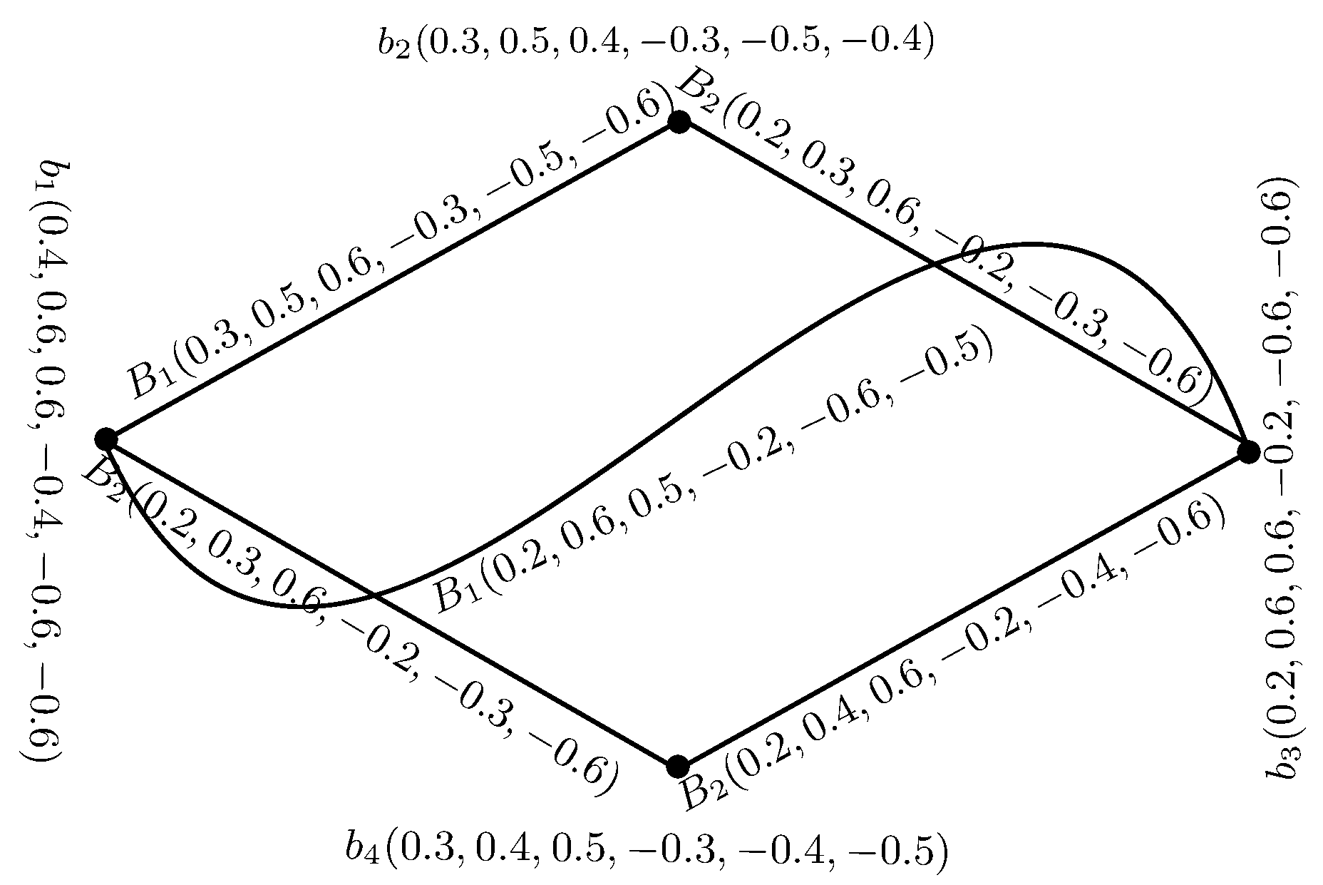
Figure 5.
A bipolar single-valued neutrosophic graph structure (BSVNGS) = .
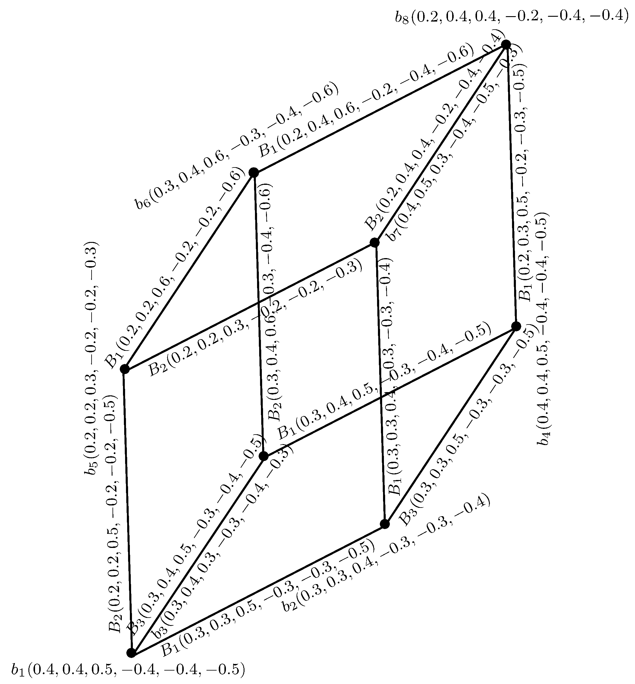
Figure 6.
A BSVNGS = .
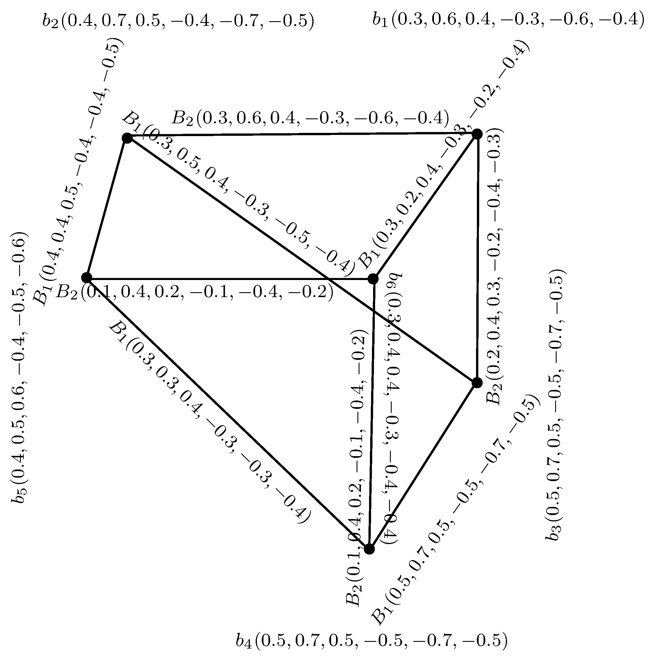
Figure 7.
A BSVNGS = .

Figure 8.
A BSVN -tree.
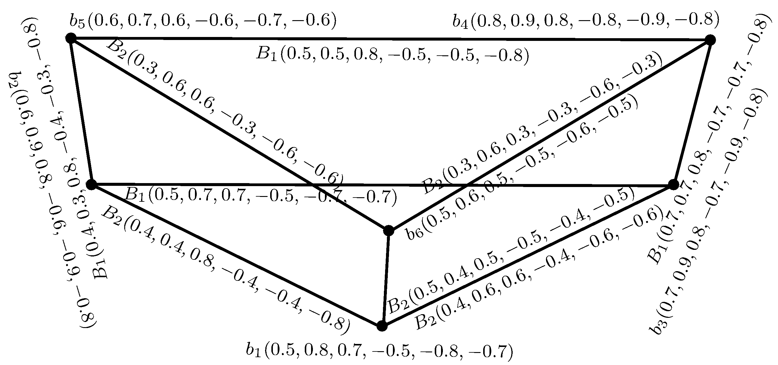
Figure 9.
A BSVN fuzzy -tree.

Figure 10.
Two BSVNGSs and .
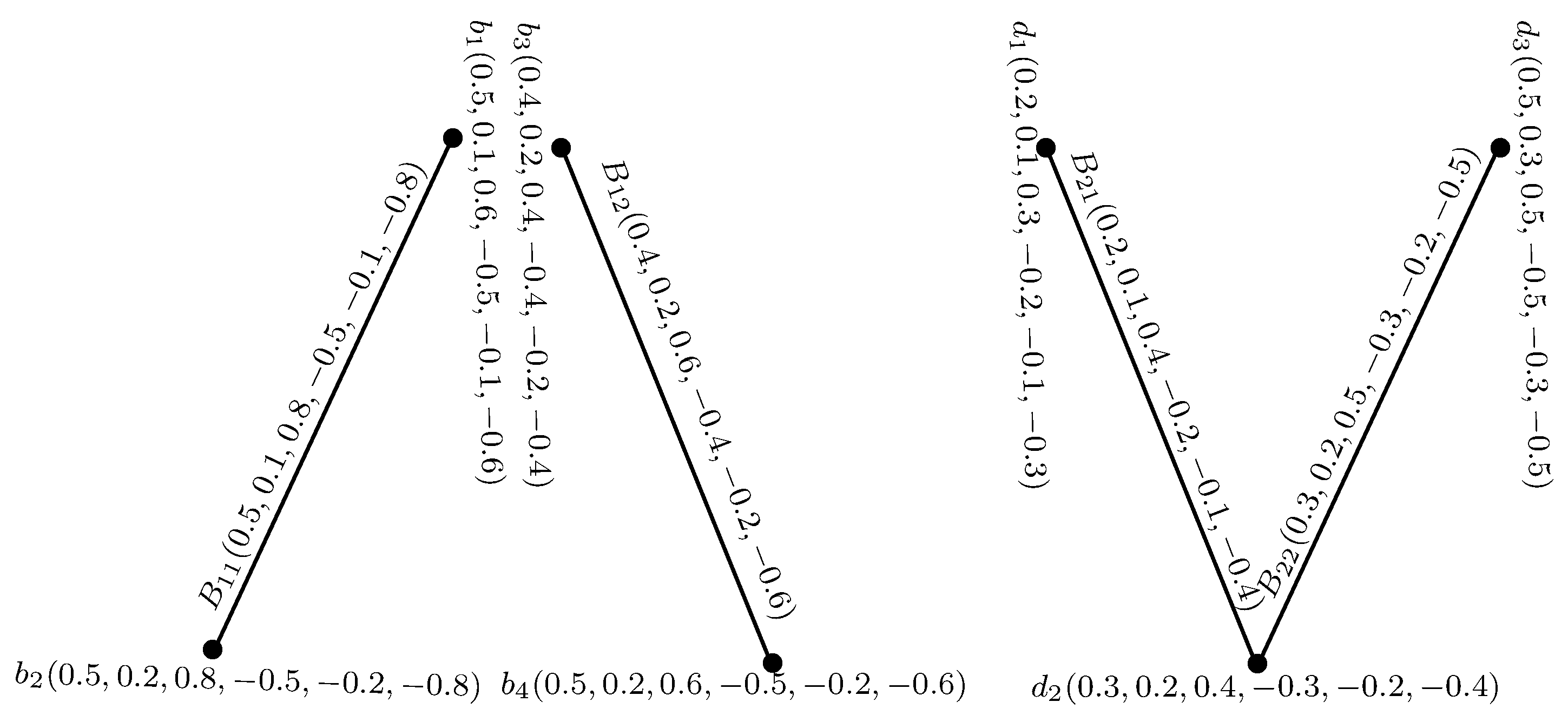
Figure 11.
.
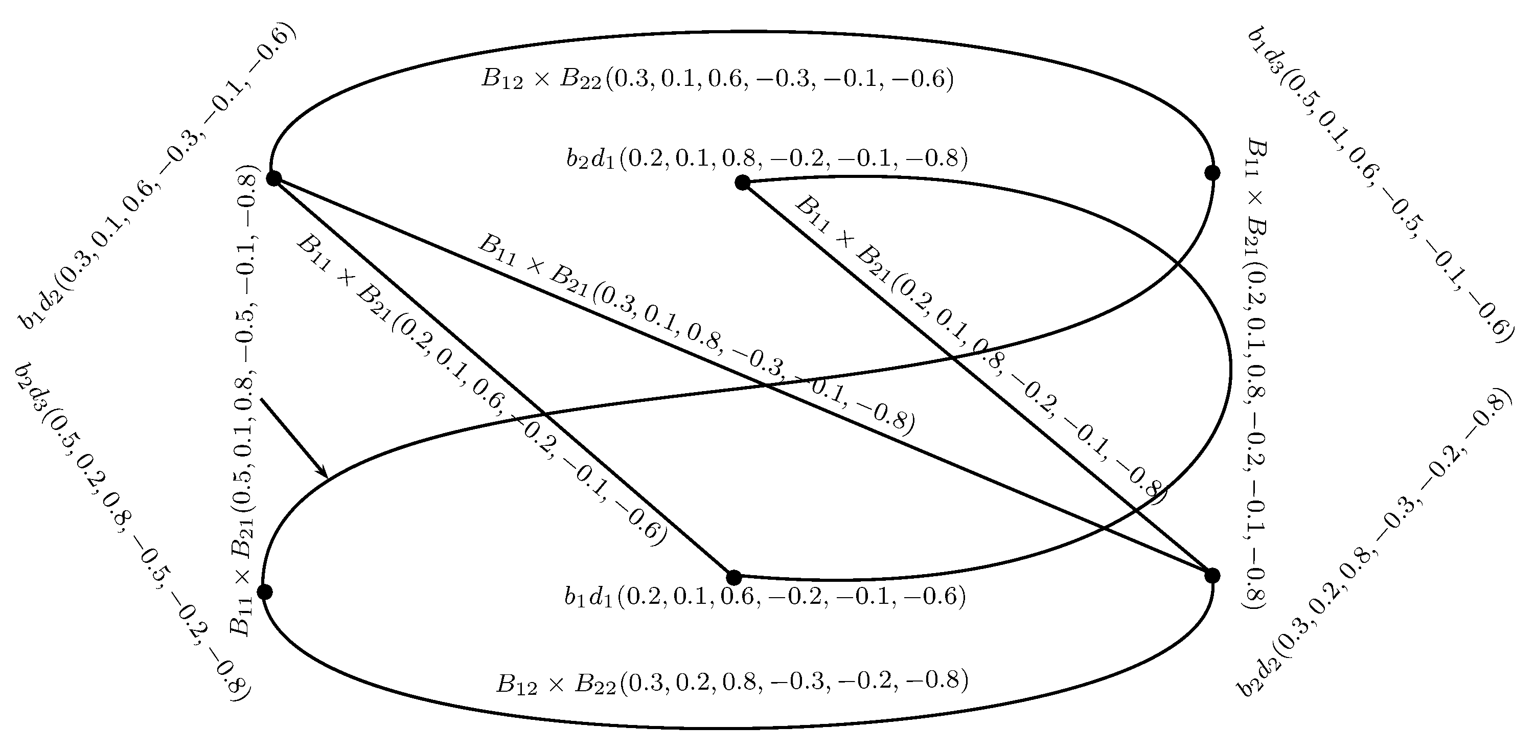
Figure 12.
.

Figure 13.
.
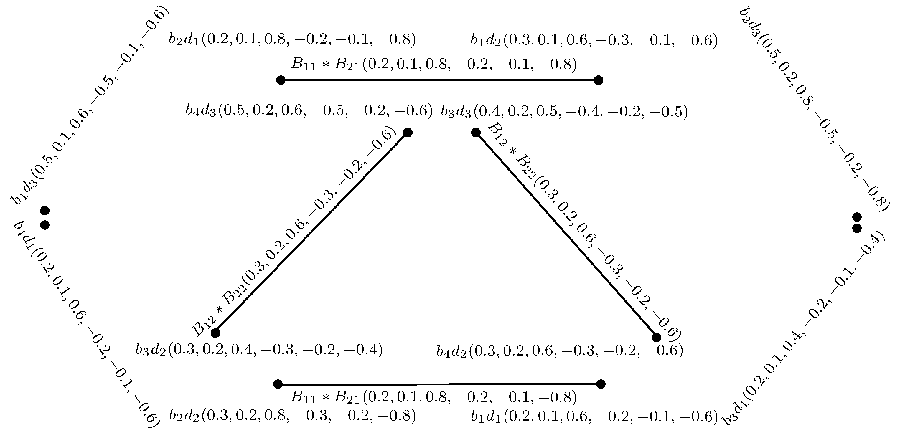
Figure 14.
.

Figure 15.
.

Table 1.
Bipolar single-valued neutrosophic (BSVN) set B on vertex set V.
| B | ||||||||
|---|---|---|---|---|---|---|---|---|
| 0.5 | 0.4 | 0.4 | 0.5 | 0.3 | 0.4 | 0.5 | 0.3 | |
| 0.4 | 0.3 | 0.4 | 0.4 | 0.2 | 0.4 | 0.5 | 0.4 | |
| 0.6 | 0.5 | 0.4 | 0.6 | 0.4 | 0.7 | 0.4 | 0.5 | |
| −0.5 | −0.4 | −0.4 | −0.5 | −0.3 | −0.4 | −0.5 | −0.3 | |
| −0.4 | −0.3 | −0.4 | −0.4 | −0.2 | −0.4 | −0.5 | −0.4 | |
| −0.6 | −0.5 | −0.4 | −0.6 | −0.4 | −0.7 | −0.4 | −0.5 |
Table 2.
BSVN sets , and .
| 0.4 | 0.4 | 0.3 | 0.3 | 0.3 | 0.4 | 0.3 | 0.3 | 0.4 | 0.3 | 0.4 | 0.4 | |||
| 0.3 | 0.3 | 0.4 | 0.4 | 0.2 | 0.4 | 0.2 | 0.2 | 0.4 | 0.4 | 0.4 | 0.3 | |||
| 0.6 | 0.5 | 0.6 | 0.7 | 0.7 | 0.6 | 0.6 | 0.4 | 0.7 | 0.5 | 0.6 | 0.6 | |||
| −0.4 | −0.4 | −0.3 | −0.3 | −0.3 | −0.4 | −0.3 | −0.3 | −0.4 | −0.3 | −0.4 | −0.4 | |||
| −0.3 | −0.3 | −0.4 | −0.4 | −0.2 | −0.4 | −0.2 | −0.2 | −0.4 | −0.4 | −0.4 | −0.3 | |||
| −0.6 | −0.5 | −0.6 | −0.7 | −0.7 | −0.6 | −0.6 | −0.4 | −0.7 | −0.5 | −0.6 | −0.6 |
© 2017 by the authors. Licensee MDPI, Basel, Switzerland. This article is an open access article distributed under the terms and conditions of the Creative Commons Attribution (CC BY) license (http://creativecommons.org/licenses/by/4.0/).
Share and Cite
MDPI and ACS Style
Akram, M.; Sitara, M.; Smarandache, F. Graph Structures in Bipolar Neutrosophic Environment. Mathematics 2017, 5, 60. https://doi.org/10.3390/math5040060
AMA Style
Akram M, Sitara M, Smarandache F. Graph Structures in Bipolar Neutrosophic Environment. Mathematics. 2017; 5(4):60. https://doi.org/10.3390/math5040060
Chicago/Turabian StyleAkram, Muhammad, Muzzamal Sitara, and Florentin Smarandache. 2017. "Graph Structures in Bipolar Neutrosophic Environment" Mathematics 5, no. 4: 60. https://doi.org/10.3390/math5040060
Note that from the first issue of 2016, this journal uses article numbers instead of page numbers. See further details here.