Krylov Implicit Integration Factor Methods for Semilinear Fourth-Order Equations

Department of Applied and Computational Mathematics and Statistics, University of Notre Dame, Notre Dame, IN 46556, USA
*
Author to whom correspondence should be addressed.
Mathematics 2017, 5(4), 63; https://doi.org/10.3390/math5040063
Submission received: 26 September 2017
/
Revised: 7 November 2017
/
Accepted: 8 November 2017
/
Published: 16 November 2017
(This article belongs to the Special Issue Numerical Methods for Partial Differential Equations)
Abstract
:Implicit integration factor (IIF) methods were developed for solving time-dependent stiff partial differential equations (PDEs) in literature. In [Jiang and Zhang, Journal of Computational Physics, 253 (2013) 368–388], IIF methods are designed to efficiently solve stiff nonlinear advection–diffusion–reaction (ADR) equations. The methods can be designed for an arbitrary order of accuracy. The stiffness of the system is resolved well, and large-time-step-size computations are achieved. To efficiently calculate large matrix exponentials, a Krylov subspace approximation is directly applied to the IIF methods. In this paper, we develop Krylov IIF methods for solving semilinear fourth-order PDEs. As a result of the stiff fourth-order spatial derivative operators, the fourth-order PDEs have much stricter constraints in time-step sizes than the second-order ADR equations. We analyze the truncation errors of the fully discretized schemes. Numerical examples of both scalar equations and systems in one and higher spatial dimensions are shown to demonstrate the accuracy, efficiency and stability of the methods. Large time-step sizes that are of the same order as the spatial grid sizes have been achieved in the simulations of the fourth-order PDEs.
1. Introduction
Efficient and high-order accuracy temporal numerical methods are important for accurate numerical simulations of time-dependent problems. In the literature, many excellent high-order time-stepping schemes have been designed. The following are some examples: the total variation diminishing (TVD) Runge–Kutta (RK) schemes in [1,2,3,4], spectral deferred correction (SDC) methods in [5,6,7,8,9], implicit–explicit (IMEX) multistep/IMEX–RK methods in [10,11,12,13,14], hybrid methods of SDC and RK schemes [15], and so forth.
Integration factor (IF) methods are a class of “exactly linear part” time-discretization methods. They are designed for solving nonlinear partial differential equations (PDEs) whose highest spatial derivatives are linear. In IF methods, the time evolution of the stiff linear operator is performed by evaluation of the corresponding matrix exponentials. As a result, the IF-type time discretization can eliminate both the stability constraint and numerical errors in the time direction, which originate from the linear high-order spatial derivatives [16,17,18,19].
In [20], a class of efficient implicit integration factor (IIF) methods were developed to solve reaction–diffusion systems that have both stiff linear diffusion and stiff nonlinear reaction terms. The implicit terms in the schemes are free of the exponential operation of the linear terms. Therefore the exact time integration of the linear diffusion and the implicit treatment of the nonlinear reaction terms are decoupled from each other. The size of the nonlinear system resulting from the implicit treatment does not depend on the number of spatial grid points. It is only determined by the number of original PDEs. This is a novel property of the IIF methods in [20], which distinguishes IIF methods [20] from implicit exponential time-differencing (ETD) methods in [16]. IIF methods can be designed with high-order accuracy (arbitrary order of accuracy in principle) for solving stiff PDE problems, and they have large stability regions because of the implicit nature of the schemes.
To overcome the challenge of implementing IF-type methods for high-spatial-dimension problems, compact IIF methods [21] were developed for spatial discretizations on rectangular meshes. In [22], compact IIF methods were designed to solve problems in curvilinear coordinates, such as polar and spherical coordinates. These were further extended to solve more complicated high-dimensional systems in [23,24] using efficient tools such as sparse grid techniques. In [25], compact IIF methods were designed to solve semilinear fourth-order PDEs.
Another approach to efficiently apply IIF methods in solving high-dimensional problems is the Krylov subspace approximation method. In [26], the Krylov IIF methods were developed for spatial discretizations on general unstructured meshes to handle complex domain geometries. We analyzed the computational complexity of the Krylov IIF methods in [27] and found that the Krylov subspace approximation approach is especially efficient for solving high-dimensional problems with cross-derivative diffusion terms. In [28], we developed the Krylov IIF methods on sparse grids to solve high-dimensional convection–diffusion equations and achieved much more efficient algorithms than in our previous work.
Nonlinear stiff advection–diffusion–reaction (ADR) systems of equations [29] are common second-order PDE models in applications from biology, chemistry and physics. They often have nonlinear advection and reaction terms. In many complicated applications, advection- and diffusion-dominated cases may be mixed in the time-dependent ADR systems. For example, nonlinear advection can dominate at early times in the system, and later the diffusion may become dominant [30]. In [31], operator splitting compact IIF methods were designed to solve stiff ADR systems. The multistep and single-step Krylov IIF methods were developed to solve stiff ADR systems in [32,33]. The Krylov IIF methods for solving stiff ADR systems can be designed for an arbitrary order of accuracy. The stiffness of the system is resolved well, and large-time-step-size computations are obtained.
In this paper, we develop Krylov IIF methods for solving semilinear fourth-order PDEs. As a result of the stiff fourth-order spatial derivative operators, the fourth-order PDEs have much stricter constraints in time-step sizes than the second-order ADR equations. Usually these are solved by implicit schemes in order to obtain large time-step sizes. However, for traditional implicit schemes, a large coupled linear or nonlinear algebraic system needs to be solved at every time-step. Furthermore, advanced preconditioning techniques often have to be developed in order to improve the convergence of algebraic solvers for fast algorithms. In [28,33,34], IIF methods were compared to some traditional implicit schemes, and it was found that IIF methods provide an efficient approach suitable for solving PDE problems with high-order derivatives.
The semilinear fourth-order PDEs have the following general form:
where u is the unknown function, are flux functions of advection terms, are diffusion terms with coefficients and , and r is the reaction term. The coefficient of the fourth-order derivatives satisfies the condition for the well-posedness of the PDE. Advection and reaction terms are often nonlinear in the models from applications. We apply the method of lines (MOL) approach to the PDE (1). For nonlinear advection terms, a nonlinearly stable discretization for hyperbolic equations such as the third-order finite difference weighted essentially non-oscillatory (WENO) scheme with Lax–Friedrichs flux splitting [35] is used. Depending on the accuracy order of IIF time discretization, the second- or fourth-order central finite difference scheme is used to discretize the diffusion terms. Then we have a semi-discretized ODE system:
Here , , and . N is the total number of grid points. C is the approximation matrix for the linear diffusion operators by the second- or fourth-order central finite difference schemes. Hence is the approximation for the diffusion terms by the finite difference schemes, and each of their components is a linear function of numerical values on the approximation stencil. is the third-order finite difference WENO approximation for the nonlinear advection. Each of its components is a nonlinear function of the numerical values on the third-order WENO approximation stencil [36]. is the nonlinear reaction, and each of its components is a nonlinear function that depends on numerical values at one grid point.
We follow the same idea as in [32] for the second-order equations to solve the fourth-order equation (1). The rest of the paper is organized as follows. In Section 2, we derive and formulate the Krylov IIF methods for semilinear fourth-order equations. The linear error analysis is performed for the fully discretized schemes; namely, both spatial and temporal discretization errors are analyzed. Numerical experiments are presented in Section 3. Conclusions are given in Section 4.
2. High-Order Krylov IIF Methods for Fourth-Order Equations
In this section we describe the numerical methods in detail.
2.1. Spatial Discretization
For diffusion terms, central differences are used. For example, second-order approximations to diffusion terms defined on a two-dimensional spatial domain at a grid point have the following forms:
Fourth-order approximations are
In this paper, the second-order approximations to diffusion terms are used with the second-order Krylov IIF scheme, and the fourth-order approximations to diffusion terms are coupled with the third-order Krylov IIF scheme. If there are advection terms in the equation, the third-order finite difference WENO scheme with Lax–Friedrichs flux splitting [36] is applied for discretizing the nonlinear advection terms. For example, for the advection terms defined on a two-dimensional spatial domain, the conservative finite difference schemes we use approximate the point values at a uniform (or smoothly varying) grid in a conservative fashion. Namely, the derivative at is approximated along the line by a conservative flux difference:
We first consider the case of positive wind, namely, for the scalar equation, or the corresponding eigenvalue is positive for the system with a local characteristic decomposition. For the third-order WENO scheme, the numerical flux depends on three-point stencil values , . For simplicity of notation, we use to denote the value of the numerical solution u at the point along the line with the understanding that the value could be different for different y coordinates. The numerical flux is written as a convex combination of two second-order numerical fluxes based on two different substencils of two points each, and the combination coefficients depend on a “smoothness indicator” measuring the smoothness of the solution in each substencil. The detailed formulae is
where
Here, and are called the “linear weights”, and and are called the “smoothness indicators”; is a small positive number chosen to avoid the denominator becoming 0. We take in this paper.
When the wind is negative (i.e., when ), the right-biased stencil with numerical values and is used to construct a third-order WENO approximation to the numerical flux . The formulae for negative and positive wind cases are symmetric with respect to the point . For the general case of , we perform the “Lax–Friedrichs flux splitting”:
where ; is the positive wind part, and is the negative wind part. Corresponding WENO approximations have been applied to find numerical fluxes and , respectively. See [35,36] for more details.
Similar procedures are applied to the other spatial directions for advection terms and diffusion terms.
2.2. Krylov IIF Temporal Discretization
2.2.1. IIF Schemes
IIF methods for Equation (2) are constructed by exactly integrating the linear part of the system. Multiplying Equation (2) by the IF and integrating over one time-step from to , we obtain
The linear term has been integrated exactly in the time direction; thus the stiffness caused by the linear operator is eliminated. Two of the nonlinear terms in Equation (9) have different properties. The nonlinear reaction is a local term but is often stiff. The nonlinear term is derived from WENO approximations to the advection term. It is nonstiff but couples numerical values at grid points of the WENO stencil. Therefore different methods are used to deal with these and to avoid solving a large coupled nonlinear system at every time-step; this is similar to the procedure in [32].
The stiff nonlinear reaction term is approximated implicitly by a th-order Lagrange polynomial with interpolation points at . We denote , , for . The interpolation points are represented by , . We define to be the numerical solution for . The first r points are used for an implicit approximation of the nonlinear reaction term:
The nonstiff advection term is highly nonlinear as a result of the WENO approximations. Differently from the nonlinear reaction term, we approximate the nonlinear term in Equation (9) by a th-order Lagrange polynomial with interpolation points at . Hence it is approximated explicitly:
Combining Equations (9)–(11), we obtain the rth-order IIF scheme for semilinear fourth-order PDEs (Equation (1)):
where the coefficients are given by
Specifically, the second-order scheme (IIF2) is of the following form:
where
The third-order scheme (IIF3) is
where
and
2.2.2. Krylov IIF Schemes
For solving PDEs defined on two- or higher-spatial-dimension domains, directly computing and storing exponential matrices in IIF schemes is very expensive and impractical for a typical computer. Additionally, time-step sizes in the IIF schemes for fourth-order PDEs (Equations (12), (15) and (16)) can be non-uniform in general. Hence at every time-step, we need to find the products of matrix exponentials and vectors. In order to efficiently implement the IIF schemes for fourth-order PDEs (Equations (12), (15) and (16)), we use the Krylov subspace method [37,38] to approximate the product of a matrix exponential and a vector. This approach has been used in the Krylov IIF schemes for solving reaction–diffusion systems and convection–diffusion equations [26,27,28,32,33]. Here we briefly describe how to use the Krylov subspace approximation to compute the product of a matrix exponential and a vector (e.g., ). The large sparse matrix C is projected to the Krylov subspace:
The dimension M of the Krylov subspace is much smaller than the dimension N of the large sparse matrix C. The well-known Arnoldi algorithm [39] generates an orthonormal basis of the Krylov subspace and an upper Hessenberg matrix . This very small Hessenberg matrix represents the projection of the large sparse matrix C to the Krylov subspace with respect to the basis . Because the columns of are orthonormal, we have the following approximation:
where and denotes the first column of the identity matrix . Thus the large matrix exponential problem is replaced with a much smaller problem. The small matrix exponential is computed using a scaling and squaring algorithm with a Pad approximation with the only computational cost of (see [26,37,38]). Applying the Krylov subspace approximation Equation (18) to Equation (12), we obtain the rth-order Krylov IIF scheme for fourth-order PDEs:
where , and are the orthonormal basis and upper Hessenberg matrix generated by the Arnoldi algorithm with the initial vector ; , and are orthonormal basis and upper Hessenberg matrix generated by the Arnoldi algorithm with the initial vector ; , and are the orthonormal basis and upper Hessenberg matrix generated by the Arnoldi algorithm with the initial vectors , for . We note that , and are orthonormal bases of different Krylov subspaces for the same matrix C, which are generated with different initial vectors in the Arnoldi algorithm. The value of M is taken to be large enough such that the errors of Krylov subspace approximations are much less than the truncation errors of the numerical schemes (Equation (12)). From our numerical experiments in this paper, we can see that our numerical schemes have already given a clear accuracy order with very small sizes , and M does not need to be increased when the spatial–temporal resolution is refined. Specifically, the second-order Krylov IIF scheme has the following form:
where , and are the orthonormal basis and upper Hessenberg matrix generated by the Arnoldi algorithm with the initial vector ; , and are the orthonormal basis and upper Hessenberg matrix generated by the Arnoldi algorithm with the initial vector . The third-order Krylov IIF scheme has the following form:
where , and are the orthonormal basis and upper Hessenberg matrix generated by the Arnoldi algorithm with the initial vector ; , and are the orthonormal basis and upper Hessenberg matrix generated by the Arnoldi algorithm with the initial vector ; , and are the orthonormal basis and upper Hessenberg matrix generated by the Arnoldi algorithm with the initial vector . See Equation (16) for values of and .
As is pointed out in [32], in the implementation of the methods, we do not store matrices C, because only multiplications of matrices C with vectors are needed in the methods, and they correspond to certain finite difference operations. In the Krylov IIF schemes (Equations (19)–(21)) for fourth-order PDEs, the “local implicit” property of the original IIF schemes in [20] is preserved well; namely, the implicit terms are free of the exponential operation. As a result, the implicit nonlinear system is decoupled for each spatial grid point. The size of the implicit nonlinear system at every spatial grid point only depends on the number of original PDEs. This “local implicit” property provides a key factor for the efficiency of our high-order Krylov IIF schemes. The small-size implicit nonlinear system can be either solved analytically or efficiently solved numerically by a fixed-point iteration method [20] or a Newton iteration method [26].
2.3. Linear Error Analysis
In this section, we perform linear error analysis for the fully discretized linear schemes. Differently from our previous work (e.g., [32]) in which only the temporal discretization errors by the IIF schemes are analyzed, we consider both spatial and temporal discretization errors here.
For the linear analysis, we consider the linear fourth-order PDE of one spatial dimension:
where and R are constant coefficients, and . For the purpose of linear error analysis, a third-order linear upwind scheme that serves as the base scheme for the nonlinear third-order WENO scheme,
is applied for discretizing the advection term.
For the IIF2 scheme (Equation (15)), the second-order central differences are used to discretize the diffusion terms in Equation (22). The matrix C in the IIF2 scheme (Equation (15)) has the following form:
We apply the IIF2 scheme (Equation (15)) to the PDE (Equation (22)) and replace the exponential terms by their Taylor expansions. For example,
IIF schemes are exponential integrator-type schemes and they are global. For a global scheme, a numerical value at the time level depends on all numerical values at the last time level . In order to derive the leading-order terms of both temporal and spatial truncation errors, we localize the IIF schemes. Four terms in the Taylor expansion (Equation (23)) are taken, and a general component is written out for the IIF2 scheme (Equation (15)). Then we find out the linear scheme for in terms of the related numerical values in the neighborhood of the spatial grid point at the time level . Because we use finite terms in the Taylor expansion (Equation (23)) to replace the matrix exponentials in the IIF schemes, the IIF schemes are localized and depends on a finite number of numerical values around , instead of all numerical values at the time level . Here we perform a linear analysis using the PDE (Equation (22)) with constant coefficients, so that the time step sizes in IIF schemes are uniform. We denote the uniform time step sizes by . Then a standard truncation error analysis for finite difference schemes can be carried out for the localized IIF schemes. We substitute the exact solution of the PDE (Equation (22)) into the localized IIF2 scheme and use Taylor expansions of at the point . The PDE (Equation (22)) is used repeatedly to cancel equivalent terms. As a result, we obtain
Using the original Equation (22), we derive that the leading-order terms of the truncation errors in the temporal direction for the IIF2 scheme (Equation (15)) are , while the leading-order terms of the truncation errors in the spatial direction are . It is observed that only the advection and reaction terms contribute to the truncation errors in the time direction. This analysis confirms that the numerical errors in the temporal direction, which are from the high-order derivatives (here the fourth- and second-order diffusion terms), have been removed completely, because the differential matrix from the high-order spatial derivatives is integrated exactly in the time evolution. In the spatial direction, numerical errors from the second-order discretizations for the fourth- and second-order diffusion terms dominate, as the third-order upwind scheme is used to discretize the advection term.
For the IIF3 scheme (Equation (16)), a similar analysis is performed. The fourth-order central differences are used to discretize the diffusion terms in Equation (22). The advection term is still discretized by the third-order upwind scheme, as for the IIF2 scheme. Five terms in the Taylor expansion (Equation (23)) are taken to approximate the matrix exponentials and to localize the IIF3 scheme. Then a standard truncation error analysis is performed for the localized IIF3 scheme, which leads to the following equation:
Again, using the original Equation (22), we derive that the leading-order terms of the truncation errors in the temporal direction for the IIF3 scheme (Equation (16)) are
while the leading order terms of the truncation errors in the spatial direction are . Similarly to for the IIF2 scheme, only the advection and reaction terms contribute to the truncation errors in the time direction, because the differential matrix from the high-order spatial derivatives is integrated exactly in the time evolution. In the spatial direction, numerical errors from the third-order upwind scheme to discretize the advection term dominate, as the fourth-order schemes are used for the fourth- and second-order diffusion terms.
Remark 1.
Here we have derived the leading-order terms of the truncation errors for IIF schemes. For Krylov IIF schemes, by the analysis in [37,40], Krylov approximation errors for computing matrix exponentials decay exponentially with respect to the square of the Krylov subspace dimension M. Hence with a small Krylov subspace dimension M, we observe in our numerical experiments that Krylov approximation errors are much smaller than the truncation errors of IIF schemes.
3. Numerical Experiments
In this section, we present numerical examples to show the stability, accuracy and efficiency of the Krylov IIF methods for solving semilinear fourth-order PDEs. The methods are first tested on one-spatial-dimension problems, including a Cahn–Hilliard equation and a Kuramoto–Sivashinsky (KS) equation; then multidimensional problems are solved. The Krylov subspace dimensions M are much smaller than the original matrix sizes to achieve both efficient computations for high-spatial-dimension problems and desired accuracy orders of the schemes. From the numerical experiments, we can observe that large time-step sizes, which are of the same order as the spatial grid sizes , have been achieved in numerical computations of fourth-order PDEs.
Example 1 (One-dimensional linear Cahn–Hilliard equation).
This example is from [41]. Consider a one-dimensional Cahn–Hilliard equation:
with periodic boundary conditions. By taking , , and , we obtain a linear Cahn–Hilliard equation:
The initial condition is taken to be . The exact solution of the equation is
The computation has been carried up to , at which the and errors have been measured. Errors and numerical orders of accuracy of the IIF2 and IIF3 methods are reported in Table 1. We can observe that we obtained desired accuracy orders for both schemes. In the computation, the time-step size was . This was consistent with our goal of using a large time-step size proportional to the spatial grid size for a stable and accurate computation of a fourth-order PDE. It is observed from Table 1 that in the computations by the IIF3 scheme, the spatial numerical errors dominated; thus a fourth-order rate of convergence has been obtained. In Figure 1, the numerical solutions by the IIF2 scheme, with numbers of grid cells and , and the exact solution are plotted. The convergence of the numerical solutions is clearly observed.
Example 2 (KS Equation).
We consider an example of the one-dimensional KS equations from [42]:
with the exact solution
Here and are constants chosen as in [42]:
The exact solution at has been taken to be the initial condition. Exact boundary conditions have been applied. The computation has been carried up to , at which the and errors have been measured. Numerical errors and orders of accuracy of the IIF3 and Krylov IIF3 methods are reported in Table 2. The third-order WENO scheme has been used for discretizing the nonlinear hyperbolic term in the KS equations here. The Krylov subspace dimension M has been taken to be 50 in the Krylov IIF3 scheme, and similar numerical errors were obtained to that of the IIF3 scheme. Third-order accuracy was obtained for both schemes when the mesh was refined. The time-step sizes were chosen such that the CFL number for the hyperbolic term was , because of the explicit treatment of the hyperbolic term in the schemes. Again, the time-step sizes were . Therefore large time-step sizes proportional to the spatial grid size for a stable and accurate computation of the fourth-order nonlinear KS equation have been achieved. We measured CPU times of the simulations by the IIF3 and the Krylov IIF3 schemes. When the mesh was refined, significant CPU time savings were observed. For this example, if , it took s for the IIF3 scheme to finish the simulation, while only s was needed for the Krylov IIF3 scheme. If , the IIF3 scheme needed s to finish the simulation, while the Krylov IIF3 scheme only needed s.
In the left picture of Figure 2, we present the numerical solutions of Equation (29) at the final time , using the IIF2 scheme with . The CFL number for the hyperbolic term was taken to be . The convergence of the numerical solutions to the exact solution is clearly observed. We can see that the large gradient of the solution is resolved very well by the IIF2 scheme with the WENO spatial discretization for the nonlinear term.
The KS equation is one of the simplest PDEs that can exhibit chaotic behavior [43]. We use an example from [18] to show this. The problem is given by
with periodic boundary conditions. The Krylov IIF2 scheme with has been applied in solving the problem. The spatial resolution was , and the CFL number for the hyperbolic term was . In the right picture of Figure 2, we show the time evolution for the equation from to 150. Applying the plotting technique in [18], we observed the interesting chaotic behavior simulated by our Krylov IIF2 scheme coupled with the WENO scheme, as shown in Figure 2.
Example 3 (A two-dimensional scalar equation).
This example is from [25]. Consider the following two-dimensional fourth-order PDE:
with periodic boundary conditions. The exact solution of the problem is
We first used this simple two-dimensional problem to test the performance of our Krylov type IIF schemes in handling high-spatial-dimension fourth-order PDEs. The computation has been carried up to , at which the and errors have been measured. The CPU time, numerical errors and numerical orders of accuracy of the Krylov IIF2 scheme with second-order approximations to the diffusion terms, as well as the Krylov IIF3 scheme with fourth-order approximations to the diffusion terms, are reported in Table 3. We can observe that we obtained the desired accuracy orders for both schemes. In the computations by the Krylov IIF3 scheme, the spatial numerical errors dominated; thus a fourth-order rate of convergence has been obtained. As for the one-dimensional problems, we achieved large-time-step-size simulations for this fourth-order PDE, namely, ; thus the time-step size was proportional to the spatial grid size. For this example, the Krylov subspace dimension M could be taken as small as 5, which is much smaller than the size of the matrix C, . Hence, the simulations could be performed very efficiently, as shown by the CPU times in Table 3.
Example 4 (A two-dimensinoal system of equations with stiff reactions).
In this example, we test the methods for solving problems with stiff reactions. We consider a fourth-order system of equations with stiff reactions on a two-dimensional domain . Similar examples of second-order systems of reaction–diffusion and ADR equations were constructed in [20,31,32] and used to test the IIF and Krylov IIF schemes for solving problems with stiff reactions. The fourth-order system has the following form:
with periodic boundary conditions. The initial condition is taken as
and the system has the exact solution
The parameters have been chosen as and to give stiff reaction terms. The computation has been carried up to , at which the and errors have been measured. The CPU time, numerical errors and numerical orders of accuracy of the Krylov IIF2 and the Krylov IIF3 schemes are reported in Table 4. As in previous examples, we can observe that we obtained the desired accuracy orders for both schemes. A small Krylov subspace dimension made the simulations very efficient for this two-dimensional problem, as shown in Table 4. Again, we achieved large-time-step-size simulations for this fourth-order PDE system, namely, for both schemes.
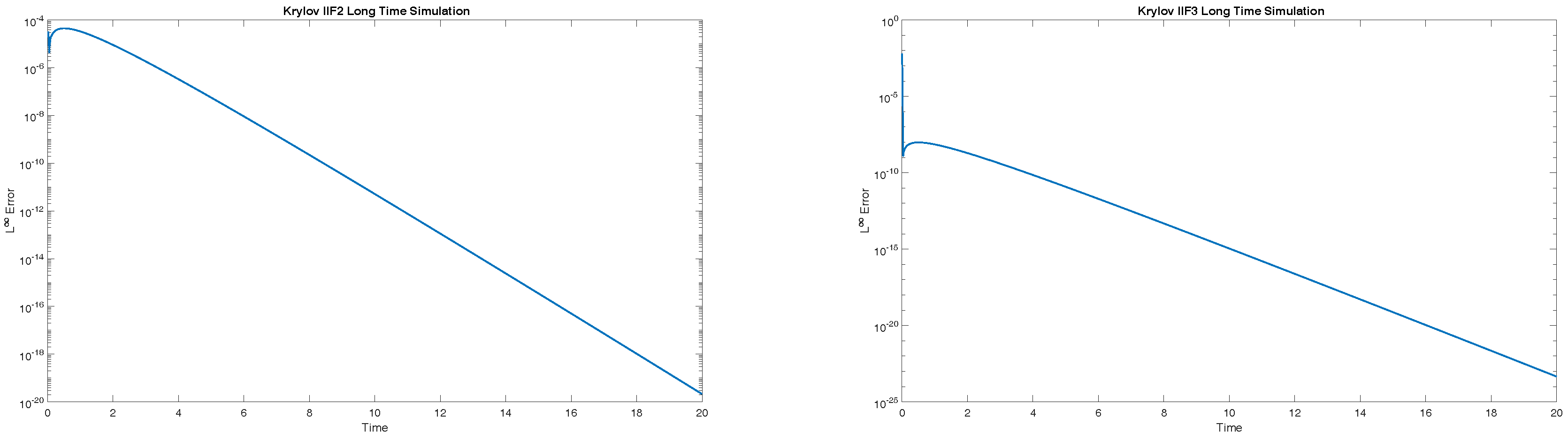
To test the methods for stiffer problems, we chose the parameters and . The ratio of eigenvalues of reaction terms was 1000, which resulted in a much stiffer system. Both the Krylov IIF2 and Krylov IIF3 schemes were tested for this case. Long time simulations, until , were performed, and the computations were stable. The history of the time integration errors in the norm for both the Krylov IIF2 and Krylov IIF3 schemes is presented in Figure 3. We observe that simulations by both schemes were stable and that the time integration errors were small.
Example 5 (A three-dimensional system of equations with stiff reactions).
We consider the three-dimensional version of Example 4, to further show the efficiency of the Krylov IIF schemes for high-spatial-dimension problems. The fourth-order system of equations defined on a three-dimensional spatial domain has the following form:
with periodic boundary conditions. For the initial condition
the system has the exact solution
The parameters have been chosen as and to give stiff reaction terms, as in Example 4. The computation has been carried up to , at which the and errors have been measured. The CPU time, numerical errors and numerical orders of accuracy of the Krylov IIF2 and the Krylov IIF3 schemes are reported in Table 5. The desired accuracy orders for both schemes have been obtained. For the Krylov IIF3 scheme, as it coupled with fourth-order approximations to the diffusion terms, we observed an approximately fourth-order convergence rate. Again, a small Krylov subspace dimension made the three-dimensional simulations very efficient, as shown in Table 5, and large-time-step-size simulations () for this three-dimensional fourth-order PDE system have been achieved for both schemes.
Example 6 (A three-dimensional fourth-order equation with nonlinear advection and reaction terms).
In this example, we test the methods for solving problems with nonlinear advection and reaction terms. The equation has the following form:
with periodic boundary conditions. Here
The exact solution of the equation is
The computation has been carried up to , at which the and errors have been measured. The third-order WENO scheme has been used to discretize the nonlinear advection terms. Newton iterations have been used to solve the nonlinear equations resulting from the implicit treatment of the reaction terms. As a result of the “local implicit” property of the IIF schemes, only one nonlinear equation needed to be solved at each grid point for this example. The CPU time, numerical errors and numerical orders of accuracy of the Krylov IIF2 and the Krylov IIF3 schemes are reported in Table 6. The desired accuracy orders for both schemes have been obtained. The time-step sizes were chosen such that the CFL number for the hyperbolic term was , because of the explicit treatment of the hyperbolic terms in the schemes. Again, the time-step sizes were ; thus large time-step sizes proportional to the spatial grid size for a stable and accurate computation of this fourth-order nonlinear equation have been achieved. For this nonlinear three-dimensional problem, we needed a higher Krylov subspace dimension than for the previous simpler problems. A Krylov subspace dimension of for the Krylov IIF2 scheme and for the Krylov IIF3 scheme enabled the Krylov subspace approximation errors to be much smaller than the numerical methods’ truncation errors, so that the desired accuracy orders of both schemes could be obtained. Although the Krylov subspace dimensions used in this example were higher than previous examples, they were still much smaller than the size of the matrix C, which was . This made the simulations feasible for the three-dimensional problems.
4. Conclusions
IIF methods are a class of efficient time-discretization methods for solving stiff PDE problems. In this paper, we design Krylov IIF methods for solving semilinear fourth-order PDEs. Strict constrains in time-step sizes in the numerical solving of stiff fourth-order PDEs are largely relaxed so that large time-step sizes proportional to the spatial grid size for stable and accurate simulations of fourth-order PDEs are achieved. Krylov subspace approximations handle high-spatial-dimension problems efficiently. Linear error analysis has been performed for the fully discretized schemes to derive both spatial and temporal discretization errors. Via numerical experiments, we verified that the methods are efficient and accurate for simulating semilinear fourth-order PDE problems. For Krylov IIF schemes, how to determine the optimal Krylov subspace dimension M, which is problem dependent, is one of the open questions. This will be part of our future work.
Acknowledgments
Research supported by NSF grant DMS-1620108.
Author Contributions
M. Machen and Y.-T. Zhang performed the research and wrote the paper.
Conflicts of Interest
The authors declare no conflict of interest.
References
- Gottlieb, S.; Shu, C.-W. Total variation diminishing Runge-Kutta schemes. Math. Comput. 1998, 67, 73–85. [Google Scholar] [CrossRef]
- Gottlieb, S.; Shu, C.-W.; Tadmor, E. Strong stability preserving high order time discretization methods. SIAM Rev. 2001, 43, 89–112. [Google Scholar] [CrossRef]
- Shu, C.-W. TVD time discretizations. SIAM J. Sci. Stat. Comput. 1988, 9, 1073–1084. [Google Scholar] [CrossRef]
- Shu, C.-W.; Osher, S. Efficient implementation of essentially non-oscillatory shock-capturing schemes. J. Comput. Phys. 1988, 77, 439–471. [Google Scholar] [CrossRef]
- Bourlioux, A.; Layton, A.T.; Minion, M.L. High-order multi-implicit spectral deferred correction methods for problems of reactive flow. J. Comput. Phys. 2003, 189, 651–675. [Google Scholar] [CrossRef]
- Dutt, A.; Greengard, L.; Rokhlin, V. Spectral deferred correction methods for ordinary differential equations. BIT Numer. Math. 2000, 40, 241–266. [Google Scholar] [CrossRef]
- Huang, J.; Jia, J.; Minion, M. Arbitrary order Krylov deferred correction methods for differential algebraic equations. J. Comput. Phys. 2007, 221, 739–760. [Google Scholar] [CrossRef]
- Layton, A.T.; Minion, M.L. Conservative multi-implicit spectral deferred correction methods for reacting gas dynamics. J. Comput. Phys. 2004, 194, 697–715. [Google Scholar] [CrossRef]
- Minion, M.L. Semi-implicit spectral deferred correction methods for ordinary differential equations. Commun. Math. Sci. 2003, 1, 471–500. [Google Scholar] [CrossRef]
- Ascher, U.; Ruuth, S.; Wetton, B. Implicit-explicit methods for time-dependent PDE’s. SIAM J. Numer. Anal. 1995, 32, 797–823. [Google Scholar]
- Kanevsky, A.; Carpenter, M.H.; Gottlieb, D.; Hesthaven, J.S. Application of implicit-explicit high order Runge-Kutta methods to Discontinuous-Galerkin schemes. J. Comput. Phys. 2007, 225, 1753–1781. [Google Scholar] [CrossRef]
- Kennedy, C.A.; Carpenter, M.H. Additive Runge-Kutta schemes for convection-diffusion-reaction equations. Appl. Numer. Math. 2003, 44, 139–181. [Google Scholar] [CrossRef]
- Verwer, J.G.; Sommeijer, B.P.; Hundsdorfer, W. RKC time-stepping for advection-diffusion-reaction problems. J. Comput. Phys. 2004, 201, 61–79. [Google Scholar] [CrossRef]
- Zhong, X. Additive semi-implicit Runge-Kutta methods for computing high-speed nonequilibrium reactive flows. J. Comput. Phys. 1996, 128, 19–31. [Google Scholar] [CrossRef]
- Christlieb, A.; Ong, B.; Qiu, J.-M. Integral deferred correction methods constructed with high order Runge-Kutta integrators. Math. Comput. 2010, 79, 761–783. [Google Scholar] [CrossRef]
- Beylkin, G.; Keiser, J.M.; Vozovoi, L. A new class of time discretization schemes for the solution of nonlinear PDEs. J. Comput. Phys. 1998, 147, 362–387. [Google Scholar] [CrossRef]
- Cox, S.M.; Matthews, P.C. Exponential time differencing for stiff systems. J. Comput. Phys. 2002, 176, 430–455. [Google Scholar]
- Kassam, A.-K.; Trefethen, L.N. Fourth-order time stepping for stiff PDEs. SIAM J. Sci. Comput. 2005, 26, 1214–1233. [Google Scholar]
- Maday, Y.; Patera, A.T.; Ronquist, E.M. An operator-integration-factor splitting method for time-dependent problems: Application to incompressible fluid flow. J. Sci. Comput. 1990, 5, 263–292. [Google Scholar] [CrossRef]
- Nie, Q.; Zhang, Y.-T.; Zhao, R. Efficient semi-implicit schemes for stiff systems. J. Comput. Phys. 2006, 214, 521–537. [Google Scholar] [CrossRef]
- Nie, Q.; Wan, F.; Zhang, Y.-T.; Liu, X.-F. Compact integration factor methods in high spatial dimensions. J. Comput. Phys. 2008, 227, 5238–5255. [Google Scholar] [CrossRef] [PubMed]
- Liu, X.F.; Nie, Q. Compact integration factor methods for complex domains and adaptive mesh refinement. J. Comput. Phys. 2010, 229, 5692–5706. [Google Scholar] [CrossRef] [PubMed]
- Wang, D.; Zhang, L.; Nie, Q. Array-representation integration factor method for high-dimensional systems. J. Comput. Phys. 2014, 258, 585–600. [Google Scholar] [CrossRef] [PubMed]
- Wang, D.; Chen, W.; Nie, Q. Semi-implicit integration factor methods on sparse grids for high-dimensional systems. J. Comput. Phys. 2015, 292, 43–55. [Google Scholar] [CrossRef] [PubMed]
- Ju, L.; Liu, X.; Leng, W. Compact implicit integration factor methods for a family of semilinear fourth-order parabolic equations. Discret. Contin. Dyn. Syst.-Ser. B 2014, 19, 1667–1687. [Google Scholar] [CrossRef]
- Chen, S.; Zhang, Y.-T. Krylov implicit integration factor methods for spatial discretization on high dimensional unstructured meshes: Application to discontinuous Galerkin methods. J. Comput. Phys. 2011, 230, 4336–4352. [Google Scholar] [CrossRef]
- Lu, D.; Zhang, Y.-T. Computational complexity study on Krylov integration factor WENO method for high spatial dimension convection-diffusion problems. J. Sci. Comput. 2017, 73, 980–1027. [Google Scholar] [CrossRef]
- Lu, D.; Zhang, Y.-T. Krylov integration factor method on sparse grids for high spatial dimension convection-diffusion equations. J. Sci. Comput. 2016, 69, 736–763. [Google Scholar] [CrossRef]
- Hundsdorfer, W.; Verwer, J. Numerical Solution of Time-Dependent Advection-Diffusion-Reaction Equations; Springer: Berlin, Germany, 2003. [Google Scholar]
- Lushnikov, P.; Chen, N.; Alber, M.S. Macroscopic dynamics of biological cells interacting via chemotaxis and direct contact. Phys. Rev. E 2008, 78. [Google Scholar] [CrossRef] [PubMed]
- Zhao, S.; Ovadia, J.; Liu, X.; Zhang, Y.-T.; Nie, Q. Operator splitting implicit integration factor methods for stiff reaction-diffusion-advection systems. J. Comput. Phys. 2011, 230, 5996–6009. [Google Scholar] [CrossRef] [PubMed]
- Jiang, T.; Zhang, Y.-T. Krylov implicit integration factor WENO methods for semilinear and fully nonlinear advection-diffusion-reaction equations. J. Comput. Phys. 2013, 253, 368–388. [Google Scholar] [CrossRef]
- Jiang, T.; Zhang, Y.-T. Krylov single-step implicit integration factor WENO methods for advection-diffusion-reaction equations. J. Comput. Phys. 2016, 311, 22–44. [Google Scholar]
- Chou, C.-S.; Zhang, Y.-T.; Zhao, R.; Nie, Q. Numerical methods for stiff reaction-diffusion systems. Discret. Contin. Dyn. Syst.-Ser. B 2007, 7, 515–525. [Google Scholar] [CrossRef]
- Shu, C.-W. Essentially Non-Oscillatory and Weighted Essentially Non-Oscillatory Schemes for Hyperbolic Conservation Laws. In Advanced Numerical Approximation of Nonlinear Hyperbolic Equations; Cockburn, B., Johnson, C., Shu, C.-W., Tadmor, E., Eds.; Springer: Berlin, Germany, 1998. [Google Scholar]
- Jiang, G.-S.; Shu, C.-W. Efficient implementation of weighted ENO schemes. J. Comput. Phys. 1996, 126, 202–228. [Google Scholar] [CrossRef]
- Gallopoulos, E.; Saad, Y. Efficient solution of parabolic equations by Krylov approximation methods. SIAM J. Sci. Stat. Comput. 1992, 13, 1236–1264. [Google Scholar] [CrossRef]
- Moler, C.; Van Loan, C. Nineteen dubious ways to compute the exponential of a matrix, twenty-five years later. SIAM Rev. 2003, 45, 3–49. [Google Scholar] [CrossRef]
- Trefethen, L.N.; Bau, D. Numerical Linear Algebra; SIAM: Philadelphia, PA, USA, 1997. [Google Scholar]
- Hochbruck, M.; Lubich, C. On Krylov subspace approximations to the matrix exponential operator. SIAM J. Numer. Anal. 1997, 34, 1911–1925. [Google Scholar] [CrossRef]
- Xia, Y.; Xu, Y.; Shu, C.-W. Local discontinuous Galerkin methods for the Cahn-Hilliard type equations. J. Comput. Phys. 2007, 227, 472–491. [Google Scholar] [CrossRef]
- Xu, Y.; Shu, C.-W. Local discontinuous Galerkin methods for the Kuramoto-Sivashinsky equations and the Ito-type coupled KdV equations. Comput. Methods Appl. Mech. Eng. 2006, 195, 3430–3447. [Google Scholar] [CrossRef]
- Hyman, J.M.; Nicolaenko, B. The Kuramoto-Sivashinsky equation: A bridge between PDEs and dynamical systems. Phys. D Nonlinear Phenom. 1986, 18, 113–126. [Google Scholar] [CrossRef]
Figure 1.
Example 1. The one-dimensional Cahn–Hilliard equation solved by the IIF2 scheme. Time: and . Solid line represents exact solution; red dots represent numerical solution with ; blue dots represent numerical solution with .
Figure 1.
Example 1. The one-dimensional Cahn–Hilliard equation solved by the IIF2 scheme. Time: and . Solid line represents exact solution; red dots represent numerical solution with ; blue dots represent numerical solution with .
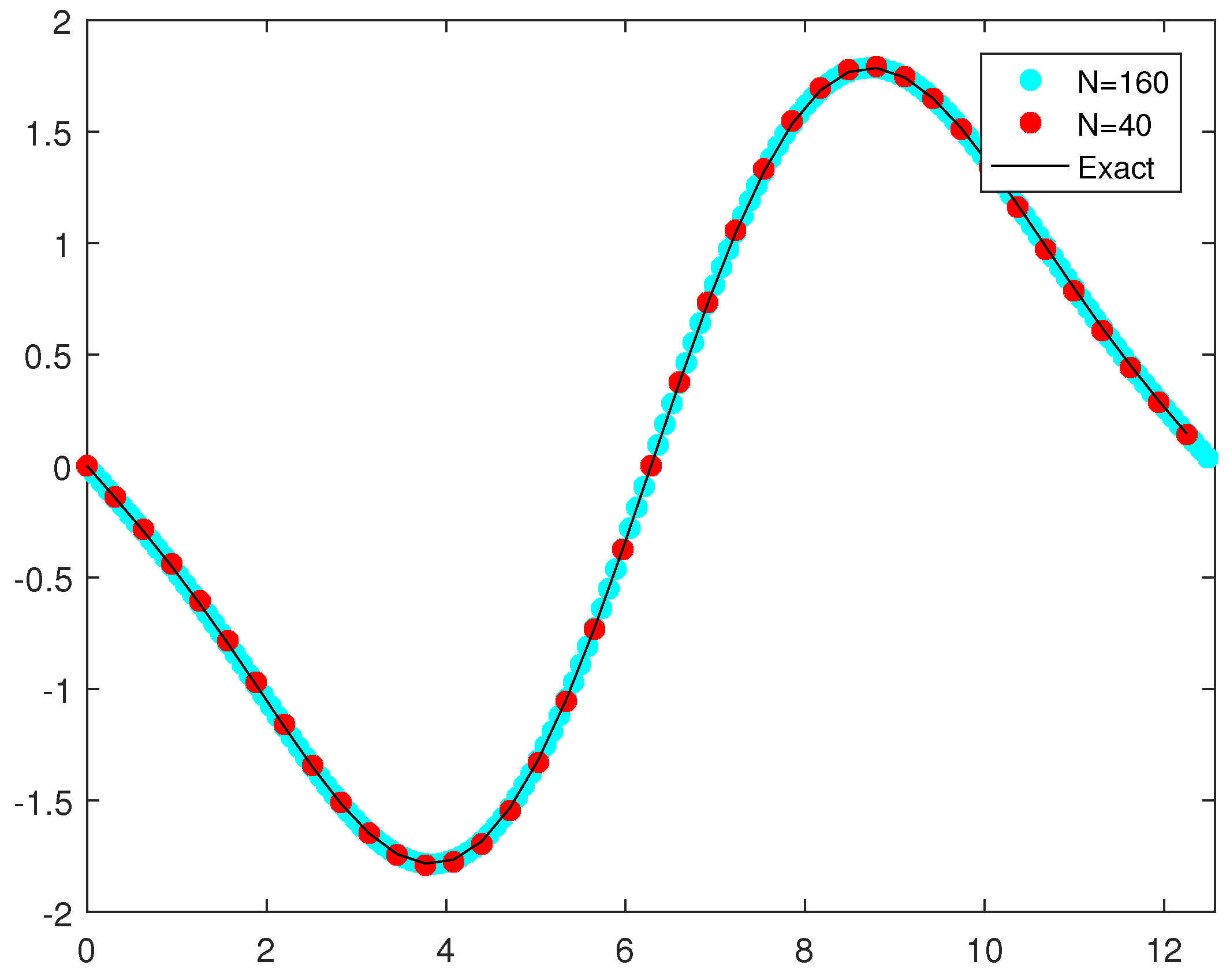
Figure 2.
Example 2. Kuramoto–Sivashinsky (KS) equations. Spatial discretizations: the third-order WENO scheme for the advection term; the second-order central schemes for diffusion terms. Left picture: numerical solutions of Equation (29) using the IIF2 scheme with ; final time: ; CFL number for the hyperbolic term: . Right picture: time evolution for Equation (32) solved using the Krylov IIF2 scheme with ; ; CFL number for the hyperbolic term: ; time runs from at the bottom of the picture to 150 at the top.

Figure 3.
Example 4. A two-dimensional system of equations with stiff reactions. Plots of history of long-period integration errors in norm for Krylov IIF2 and IIF3 schemes. The ratio of eigenvalues of reaction terms is 1000. The spatial mesh is . Time-step sizes: for Krylov IIF2 scheme and for Krylov IIF3 scheme. Krylov subspace dimension: . Simulations run from to the final time . Left picture: error history for Krylov IIF2. Right picture: error history for Krylov IIF3.


Table 1.
Example 1: Cahn–Hilliard equation. Numerical errors and orders of accuracy of the implicit integration factor (IIF)2 and IIF3 schemes; ; final time: T = 1.0.
Table 1.
Example 1: Cahn–Hilliard equation. Numerical errors and orders of accuracy of the implicit integration factor (IIF)2 and IIF3 schemes; ; final time: T = 1.0.
| IIF2 Scheme | ||||
| Error | Order | Error | Order | |
| 20 | 4.20 × 10 | — | 2.62 × 10 | — |
| 40 | 1.34 × 10 | 1.65 | 8.15 × 10 | 1.68 |
| 80 | 3.63 × 10 | 1.88 | 2.22 × 10 | 1.87 |
| 160 | 9.45 × 10 | 1.94 | 5.79 × 10 | 1.94 |
| 320 | 2.41 × 10 | 1.97 | 1.48 × 10 | 1.97 |
| IIF3 Scheme | ||||
| Error | Order | Error | Order | |
| 20 | 2.94 × 10 | — | 1.89 × 10 | — |
| 40 | 2.48 × 10 | 3.56 | 1.56 × 10 | 3.60 |
| 80 | 1.72 × 10 | 3.85 | 1.09 × 10 | 3.84 |
| 160 | 1.12 × 10 | 3.94 | 7.12 × 10 | 3.93 |
| 320 | 7.97 × 10 | 3.82 | 4.27 × 10 | 4.06 |
Table 2.
Example 2. Kuramoto–Sivashinsky (KS) Equation (29). Numerical errors and orders of accuracy of the IIF3 and Krylov IIF3 schemes. The third-order weighted essentially non-oscillatory (WENO) scheme was used for discretizing the nonlinear hyperbolic term; ; final time: T = 1.0.
Table 2.
Example 2. Kuramoto–Sivashinsky (KS) Equation (29). Numerical errors and orders of accuracy of the IIF3 and Krylov IIF3 schemes. The third-order weighted essentially non-oscillatory (WENO) scheme was used for discretizing the nonlinear hyperbolic term; ; final time: T = 1.0.
| IIF3 Scheme | ||||
| Error | Order | Error | Order | |
| 40 | 5.03 × 10 | — | 5.55 × 10 | — |
| 80 | 2.43 × 10 | 1.05 | 2.07 × 10 | 1.42 |
| 160 | 5.57 × 10 | 2.12 | 4.53 × 10 | 2.19 |
| 320 | 8.12 × 10 | 2.78 | 6.49 × 10 | 2.80 |
| 640 | 7.44 × 10 | 3.45 | 6.11 × 10 | 3.41 |
| Krylov IIF3 Scheme | ||||
| Error | Order | Error | Order | |
| 40 | 5.03 × 10 | — | 5.55 × 10 | — |
| 80 | 2.43 × 10 | 1.05 | 2.07 × 10 | 1.42 |
| 160 | 5.57 × 10 | 2.12 | 4.53 × 10 | 2.19 |
| 320 | 8.12 × 10 | 2.78 | 6.49 × 10 | 2.80 |
| 640 | 7.61 × 10 | 3.42 | 7.15 × 10 | 3.18 |
Table 3.
Example 3, a two-dimensional scalar problem. CPU time, numerical errors and orders of accuracy of the Krylov IIF2 and Krylov IIF3 schemes. Krylov subspace dimension: ; ; final time .
Table 3.
Example 3, a two-dimensional scalar problem. CPU time, numerical errors and orders of accuracy of the Krylov IIF2 and Krylov IIF3 schemes. Krylov subspace dimension: ; ; final time .
| Krylov IIF2 Scheme | |||||
| Error | Order | Error | Order | CPU Time (Seconds) | |
| 1.03 × 10 | — | 4.25 × 10 | — | 0.77 | |
| 2.44 × 10 | 2.08 | 9.88 × 10 | 2.10 | 1.44 | |
| 6.02 × 10 | 2.02 | 2.44 × 10 | 2.02 | 3.92 | |
| 1.50 × 10 | 2.00 | 6.08 × 10 | 2.00 | 22.73 | |
| Krylov IIF3 Scheme | |||||
| Error | Order | Error | Order | CPU Time (Seconds) | |
| 1.17 × 10 | — | 4.80 × 10 | — | 1.09 | |
| 7.66 × 10 | 3.93 | 3.10 × 10 | 3.95 | 2.66 | |
| 5.00 × 10 | 3.94 | 2.03 × 10 | 3.93 | 9.80 | |
| 3.36 × 10 | 3.90 | 1.36 × 10 | 3.90 | 47.11 | |
Table 4.
Example 4. Fourth-order system with stiff reaction in two-dimensions. CPU time, numerical errors and orders of accuracy of Krylov IIF2 and Krylov IIF3 schemes. Krylov subspace dimension: ; final time: .
Table 4.
Example 4. Fourth-order system with stiff reaction in two-dimensions. CPU time, numerical errors and orders of accuracy of Krylov IIF2 and Krylov IIF3 schemes. Krylov subspace dimension: ; final time: .
| Krylov IIF2, | |||||
| Error | Order | Error | Order | CPU Time (Seconds) | |
| 5.18 × 10 | — | 3.29 × 10 | — | 0.67 | |
| 1.32 × 10 | 1.97 | 8.41 × 10 | 1.97 | 1.28 | |
| 3.34 × 10 | 1.99 | 2.12 × 10 | 1.99 | 4.59 | |
| 8.38 × 10 | 1.99 | 5.34 × 10 | 1.99 | 21.30 | |
| Krylov IIF3, | |||||
| Error | Order | Error | Order | CPU Time (Seconds) | |
| 2.94 × 10 | — | 1.86 × 10 | — | 0.56 | |
| 2.11 × 10 | 3.80 | 1.34 × 10 | 3.79 | 1.80 | |
| 1.94 × 10 | 3.45 | 1.23 × 10 | 3.44 | 8.14 | |
| 2.54 × 10 | 2.93 | 1.62 × 10 | 2.93 | 36.81 | |
Table 5.
Example 5. Fourth-order system with stiff reaction in three dimensions.CPU time, numerical errors and orders of accuracy of Krylov IIF2 and Krylov IIF3 schemes. Krylov subspace dimension: . Final time: .
Table 5.
Example 5. Fourth-order system with stiff reaction in three dimensions.CPU time, numerical errors and orders of accuracy of Krylov IIF2 and Krylov IIF3 schemes. Krylov subspace dimension: . Final time: .
| Krylov IIF2 Scheme, | |||||
| Error | Order | Error | Order | CPU Time (Seconds) | |
| 7.85 × 10 | — | 5.08 × 10 | — | 0.36 | |
| 2.08 × 10 | 1.92 | 1.31 × 10 | 1.95 | 0.72 | |
| 5.35 × 10 | 1.96 | 3.40 × 10 | 1.95 | 3.61 | |
| 1.35 × 10 | 1.98 | 8.62 × 10 | 1.98 | 33.09 | |
| 3.41 × 10 | 1.99 | 2.17 × 10 | 1.99 | 482.11 | |
| Krylov IIF3 Scheme, | |||||
| Error | Order | Error | Order | CPU Time (Seconds) | |
| 4.36 × 10 | — | 2.82 × 10 | — | 1.02 | |
| 2.91 × 10 | 3.91 | 1.84 × 10 | 3.94 | 6.38 | |
| 1.82 × 10 | 4.00 | 1.15 × 10 | 3.99 | 37.63 | |
| 1.18 × 10 | 3.94 | 7.52 × 10 | 3.94 | 416.41 | |
| 9.20 × 10 | 3.68 | 5.86 × 10 | 3.68 | 6384.67 | |
Table 6.
Example 6. Fourth-order equation with nonlinear advection and reaction terms in three dimensions. CPU time, numerical errors and orders of accuracy of Krylov IIF2 and Krylov IIF3 schemes. M is the Krylov subspace dimension. Final time: .
Table 6.
Example 6. Fourth-order equation with nonlinear advection and reaction terms in three dimensions. CPU time, numerical errors and orders of accuracy of Krylov IIF2 and Krylov IIF3 schemes. M is the Krylov subspace dimension. Final time: .
| Krylov IIF2 Scheme, | ||||||
| M | Error | Order | Error | Order | CPU Time (Seconds) | |
| 60 | 1.75 × 10 | — | 9.36 × 10 | — | 2.70 | |
| 60 | 6.89 × 10 | 1.34 | 3.57 × 10 | 1.39 | 63.72 | |
| 60 | 2.05 × 10 | 1.75 | 1.06 × 10 | 1.76 | 860.14 | |
| 60 | 5.40 × 10 | 1.93 | 2.79 × 10 | 1.92 | 28436.98 | |
| Krylov IIF3 Scheme, | ||||||
| M | Error | Order | Error | Order | CPU Time (Seconds) | |
| 90 | 1.30 × 10 | — | 7.09 × 10 | — | 11.67 | |
| 90 | 1.68 × 10 | 2.94 | 8.71 × 10 | 3.03 | 445.30 | |
| 90 | 1.70 × 10 | 3.31 | 7.98 × 10 | 3.45 | 7713.33 | |
| 90 | 1.80 × 10 | 3.24 | 7.77 × 10 | 3.36 | 149777.39 | |
© 2017 by the authors. Licensee MDPI, Basel, Switzerland. This article is an open access article distributed under the terms and conditions of the Creative Commons Attribution (CC BY) license (http://creativecommons.org/licenses/by/4.0/).
Share and Cite
MDPI and ACS Style
Machen, M.; Zhang, Y.-T. Krylov Implicit Integration Factor Methods for Semilinear Fourth-Order Equations. Mathematics 2017, 5, 63. https://doi.org/10.3390/math5040063
AMA Style
Machen M, Zhang Y-T. Krylov Implicit Integration Factor Methods for Semilinear Fourth-Order Equations. Mathematics. 2017; 5(4):63. https://doi.org/10.3390/math5040063
Chicago/Turabian StyleMachen, Michael, and Yong-Tao Zhang. 2017. "Krylov Implicit Integration Factor Methods for Semilinear Fourth-Order Equations" Mathematics 5, no. 4: 63. https://doi.org/10.3390/math5040063
Note that from the first issue of 2016, this journal uses article numbers instead of page numbers. See further details here.