Certain Algorithms for Modeling Uncertain Data Using Fuzzy Tensor Product Bézier Surfaces


Department of Mathematics, University of the Punjab, New Campus, Lahore 54590, Pakistan
*
Author to whom correspondence should be addressed.
Mathematics 2018, 6(3), 42; https://doi.org/10.3390/math6030042
Submission received: 31 January 2018
/
Revised: 5 March 2018
/
Accepted: 7 March 2018
/
Published: 9 March 2018
(This article belongs to the Special Issue Fuzzy Mathematics)
Abstract
:Real data and measures are usually uncertain and cannot be satisfactorily described by accurate real numbers. The imprecision and vagueness should be modeled and represented in data using the concept of fuzzy numbers. Fuzzy splines are proposed as an integrated approach to uncertainty in mathematical interpolation models. In the context of surface modeling, fuzzy tensor product Bézier surfaces are suitable for representing and simplifying both crisp and imprecise surface data with fuzzy numbers. The framework of this research paper is concerned with various properties of fuzzy tensor product surface patches by means of fuzzy numbers including fuzzy parametric curves, affine invariance, fuzzy tangents, convex hull and fuzzy iso-parametric curves. The fuzzification and defuzzification processes are applied to obtain the crisp Beziér curves and surfaces from fuzzy data points. The degree elevation and de Casteljau’s algorithms for fuzzy Bézier curves and fuzzy tensor product Bézier surfaces are studied in detail with numerical examples.
1. Introduction
Data points are usually collected using physical objects to capture their geometric entity and representation in a digital framework, i.e., CAGD and CAD systems. Information is collected by using particular devices such as scanning tools. However, the recorded data do not significantly describe error-free data. This is due to the fact that the errors are produced by limitations of the devices, human errors and environmental factors, etc. Generally, these sorts of data which have uncertain characteristics cannot be used directly to create digitized models. In order to make uncertain data valuable for analysis and modeling, this kind of data have to be characterized in a different approach to handle uncertainties of the measurements.
In curve designing and geometric modeling, control points play a major role in the process of controlling the shape of curves and surfaces. The issue of uncertain shape of surfaces and curves can be handled by using left, crisp, right control points through fuzzy numbers called fuzzy control points [1].
Natural spline, B-spline and Bernstein Bézier functions can be used to produce geometric models with data points [2,3,4]. The surfaces and curves produced with these functions are the standard approaches to represent a set of given data points. Tensor product Bézier surfaces, also known as Bernstein Bézier surfaces, can be determined by a collection of vertices called control points, which are joined in a sequence to form a closed or open control grid. The shape of the surface changes with the control grid in a smooth fashion. However, there is a major problem in shape designing due to uncertainty, imprecision and vagueness of the real data. The designers and experts are unable to choose an appropriate set of control points due to errors and uncertainties. One of the methods used to handle vagueness and uncertainty issues is the theory of fuzzy sets introduced in [5].
The problem of interpolation was first proposed by Zadeh in [5] stating that if for each distinct real numbers , a fuzzy value is given instead of crisp value, is it possible to construct a smooth curve to fit this fuzzy data of points? To solve Zadeh’s proposed problem, Lagrange interpolation polynomial for fuzzy data was first investigated by Lowen [6]. The problem of interpolating fuzzy data using fuzzy splines was also considered by Kaleva [7]. By using spline functions of odd degree, the interpolation of fuzzy data was considered in [8] with complete splines, in [9] with natural splines, and in [10] with fuzzy splines. The concept of a fuzzy tensor product Bézier surface was introduced in [1]. The construction of the fuzzy B-spline model, modeling of uncertain data based on B-spline model curve are discussed in [11,12,13].
In this research paper, we study various properties of fuzzy tensor product surfaces by means of fuzzy numbers including fuzzy parametric curves, affine invariance, fuzzy tangents, convex hull property and fuzzy iso-parametric curves. We also develop De Casteljau’s and degree elevation algorithms for fuzzy Beziér curves and fuzzy tensor product surfaces with numerical examples. We apply the process of fuzzification to obtain the fuzzy interval of fuzzy data points where the crisp solution exists. This is followed by the defuzzification process to construct crisp Beziér curves and surfaces which focus on the defuzzification of fuzzy data points.
We used standard definitions and terminologies in this paper. For other notations, terminologies and applications not mentioned in the paper, the readers are referred to [14,15,16,17,18,19,20,21].
Definition 1
Definition 2
([21]). A triangular fuzzy number is a fuzzy set on R, denoted by the symbol , , with membership function defined as,
The -cute operation, , of triangular fuzzy number is defined as . For any two triangular fuzzy numbers and , the sum is a triangular fuzzy number with membership function defined as, . The multiplication of by a scalar is a triangular fuzzy number whose membership function is .
Definition 3
([1]). Let Y be a space and P be a subset of control points in Y. P is said to be a collection of fuzzy control points in Y if there exists such that in which . Therefore,
with where, , are left-grade and right-grade membership values. means that partially belongs to Y. Fuzzy control points can be written as where are left fuzzy control points, crisp control points and right fuzzy control points, respectively.
Definition 4
([1]). Consider a collection of distinct fuzzy control points , , then a fuzzy Bernstein Beziér (B.B) curve is defined as,
where is kth Berstein polynomial of degree r.
Definition 5
2. Fuzzy Tensor Product Beziér Surfaces
Consider a fuzzy B.B curve,
If we define two operators on fuzzy control points, shift operator and identity operator then, Equation (1) can be written as , . This is called the symbolic representation of fuzzy B.B curve. For , a fuzzy straight line can be defined as,
where, are fuzzy control points. Consider two fuzzy B.B polynomials
where, , and , are fuzzy control points. The fuzzy tensor product surface or fuzzy Bernstein Beziér (B.B) surface can be generated using and as,
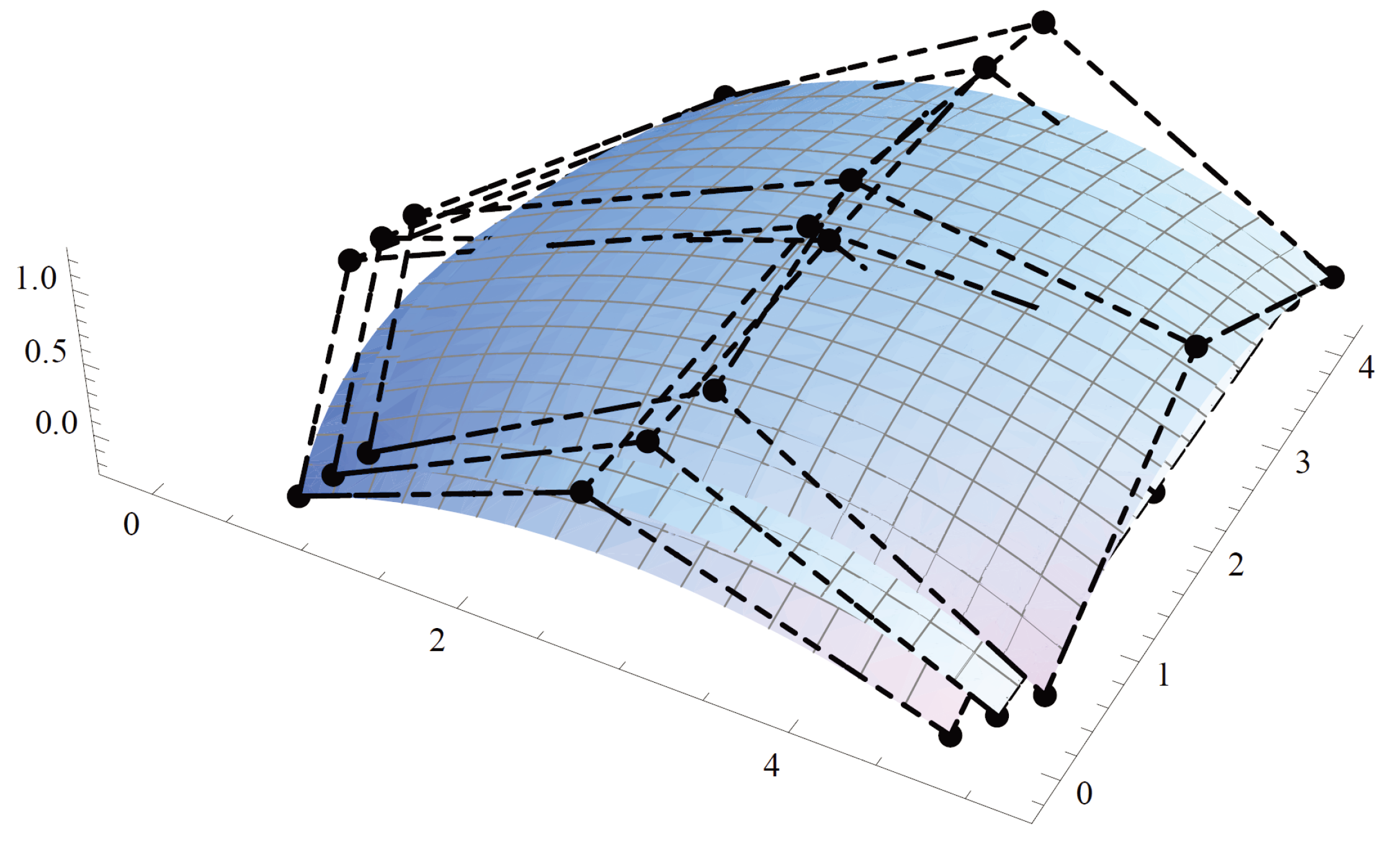
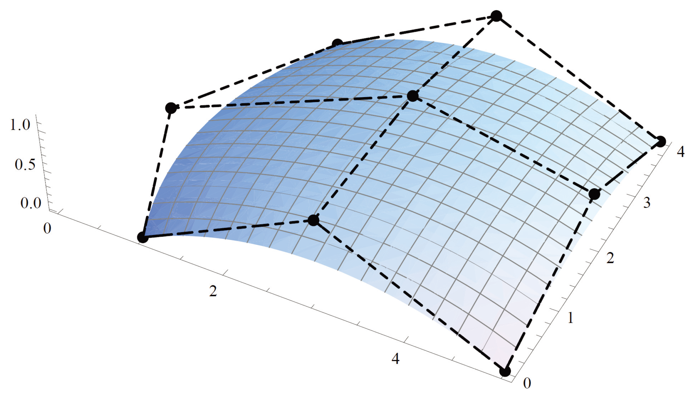
where, are fuzzy control points. For any fuzzy B.B surface, r and q are the degrees of corresponding fuzzy B.B curves. We can say that is a fuzzy B.B surface of degree . If , the fuzzy B.B surface is known as fuzzy cubic by cubic patch. Likewise, the case is called a fuzzy quadratic by quadratic patch. Also, fuzzy control points are organized into rows and columns. A fuzzy B.B surface of degree , with fuzzy control points in Table 1, is shown in Figure 1. The fuzzy control points along with dashed lines is called a fuzzy control grid of a fuzzy surface. Each column and row of the fuzzy control points interpret a fuzzy B.B curve. The fuzzy B.B curve defined by the fuzzy control points is called kth fuzzy u-curve and the fuzzy B.B curve defined by is jth fuzzy v-curve. Consequently, there are number of fuzzy u-curves and number of fuzzy v-curves. The fuzzy u-curves of Figure 1 are shown in Figure 2. The fuzzy u-curve with 0th row of fuzzy control points is shown with red lines, the 1st row of fuzzy control points is shown in blue and the 2nd row of fuzzy control points is shown in green.
In fuzzy B.B surface , and are basis functions of degree r and q, respectively. There are four fuzzy boundary curves to ,
We now present some properties of fuzzy Beziér surfaces.
- As , , and therefore, interpolates four fuzzy control points.
- and are crisp basis functions for all , , therefore, these are non-negative and .
- Let be an affine transformation where, and are sets of triangular fuzzy numbers and where, the elements of of B are triangular fuzzy numbers and is a vector of triangular fuzzy numbers. Fuzzy B.B surface satisfies affine invariance property.
- As is a linear combination of fuzzy control points with non-negative coefficients whose sum is one therefore, fuzzy B.B surface lies in the convex hull defined by the fuzzy control mesh.
- As therefore, the fuzzy tangents at the end points of fuzzy Beziér curve can be drawn using a pair of fuzzy control points. For , and for , .
- At every point of fuzzy Beziér curve, we have two fuzzy tangent directions and .
For any fuzzy B.B surface, if we fix one parameter, say , then becomes,
where, . is known as fuzzy u iso-parametric curve. Fuzzy iso-parametric curve on any fuzzy B.B surface can be obtained by fixing one parameter as constant. A fuzzy B.B surface can be considered as a family of fuzzy iso-parametric curves and these fuzzy iso-parametric curves can be studied in terms of fuzzy control curves. Figure 2 represents fuzzy u iso-parametric curves of Figure 1. For any value of a, define fuzzy control point positions for fuzzy iso-parametric curve .
Clearly, the four fuzzy iso-parametric curves are fuzzy boundary curves and . These fuzzy boundary curves are defined by rows and columns of fuzzy control points and are fuzzy control curves. For example, in Figure 1, shown in red color is a fuzzy B.B curve of degree 2 with fuzzy control points , , . Similarly, , shown in green, is a fuzzy B.B curve with fuzzy control points , , .
We now describe and design de Casteljau’s algorithm to find any point on fuzzy B.B curve.
| Algorithm 1. De Casteljau’s algorithm for fuzzy B.B curves |
Consider fuzzy B.B curve of degree r,
|
Using symbolic representation, can also be expressed as,
|
Denote and , and . Equation (2) can also be expressed as, where, and,
|
For , . |
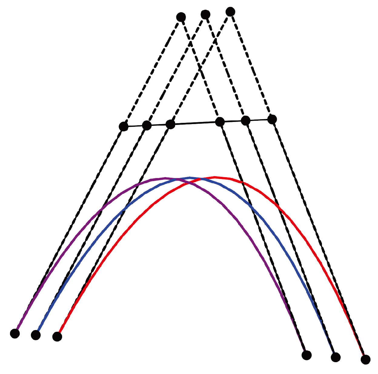
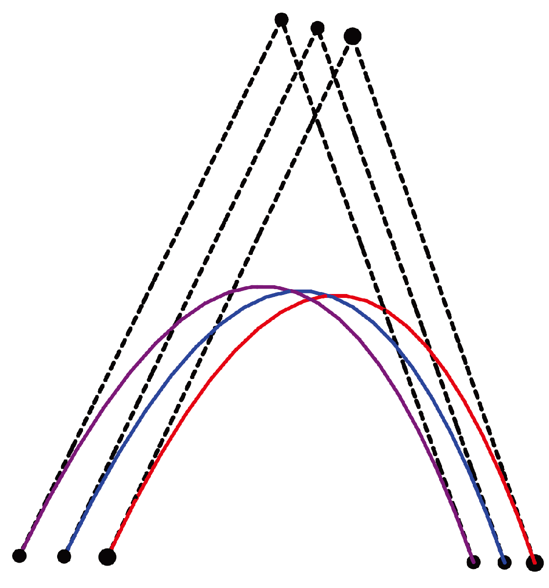
Example 1.
Consider a fuzzy cubic B.B curve, given in Figure 3, having fuzzy control points as shown in Table 2. We now find using de Casteljau’s algorithm. Clearly, where,
Similarly, , and therefore, .
| Algorithm 2. De Casteljau’s algorithm for fuzzy B.B surfaces |
Algorithm 1 can be extended to fuzzy B.B surfaces. De Casteljau’s can be implemented several times to find for particular . It is based on fuzzy iso-parametric curves. Consider the equation of fuzzy Beziér surface,
|
It clearly shows that can be calculated using fuzzy control points . The procedure can be illustrated as:
|
Example 2.
In this example, we illustrate the process of Algorithm 2 for fuzzy quadratic by quadratic surface as shown in Figure 1. We now calculate the value of for .
- Step 1: For , we compute . The fuzzy control points on the first row are , , . Applying Algorithm 2,Similarly, and .
- Step 2: Applying Algorithm 1 on all fuzzy iso-parametric curves, we obtain three fuzzy control points as shown in Table 3.
- Step 3: Applying Algorithm 2 for , we obtain the following expression,
Upon defining the fuzzy Beziér surface model, the next step is the defuzzification process. This procedure can be applied to obtain the results as a single value. For defining defuzzification, we use the -cut operation of fuzzy control points on the definition of fuzzy Beziér surface. This is called the fuzzification process, and is defined as follows.
Fuzzification process [11]:
If are the set of fuzzy control points then, is the alpa- cut of and is defined in Equation (3):
After fuzzification, the next procedure is the defuzzification of fuzzy control points to obtain the crisp solution which is described below.
Defuzzification process [11]:
The defuzzification of fuzzy control point is a crisp control point , calculated in Equation (4):
The fuzzification and defuzzification process is illustrated in Figure 4 and Figure 5. The fuzzification process is applied by means of -cut operation and a crisp Beziér surface is obtained by applying the defuzzification process.
Degree Elevation for a Fuzzy B.B Curve
Numerous applications that include more than one fuzzy B.B curve require all the fuzzy curves to have the same degree. Additionally, higher degree fuzzy B.B curves take a longer time to process, but provide more flexibility for designing shapes. The key point is to change the degree of fuzzy B.B curve without changing its shape. This process is called degree elevation. We now explain the process of degree raising for a fuzzy B.B curve.
Consider fuzzy B.B curve of degree r having fuzzy control points,
To increase the degree of fuzzy B.B curve to , fuzzy control , , are required. As the fuzzy curve passes through and therefore, the new set of fuzzy control points must include and . By replacing u by , Equation (5) can be written as,
where, , and
Each edge of fuzzy control point contains a new fuzzy control point. More precisely, edge contains in the ratio . In de Casteljau’s algorithm, the fuzzy line segment is divided in the ration . Unlike Algorithm 2, the ratio is not a constant but varies with index k.
Example 3.
Fuzzy Rational Beziér Surface Patch
A fuzzy rational Beziér curve (FRB) [13] is defined as,
where, are fuzzy weights. Fuzzy rational Beziér curves has several benefits over simple fuzzy Beziér curves. It provides large control to the shape of fuzzy curves. In addition, a 2D FRB curve can represented as a projection of a 3D fuzzy Beziér curve as,
where, , , and the operator ∏ is defined as .
The degree elevation and de Casteljau algorithm for fuzzy Beziér curve can be extended to FRB curve. For this, transform the FRB curve into a 3D fuzzy Beziér curve as discussed above. Next, apply the algorithms to 3D fuzzy Beziér curve. Finally, convert the 3D fuzzy Beziér curve to 2D fuzzy curve by applying the projection operator ∏. The resulting fuzzy control points turn out to be the fuzzy weights of given FRB curve.
3. Conclusions
Fuzzy splines are the most useful mathematical and graphical tools to reduce uncertainty in curve and surface modeling. In this research paper, various properties of fuzzy tensor product surface patches are studied using fuzzy numbers including fuzzy parametric curves, affine invariance, fuzzy tangents, convex hull and fuzzy iso-parametric curves. The degree elevation and de Casteljau’s algorithms for fuzzy Bézier curves, fuzzy tensor product Bézier surfaces and FRB curves are presented. The proposed techniques are useful to visualize uncertain and vague measures via surface modeling. The process of fuzzification is applied to obtain the fuzzy interval of fuzzy data points where the crisp solution exists. It is then followed by the defuzzification process to construct crisp Beziér curves and surfaces which are focused on the defuzzification of fuzzy data points. Finally, to check the effectiveness of Beziér surfaces this process is applied to numerical examples. We aim to extend the theory of fuzzy splines to find its applications in geometric modeling, representing fuzzy data points using fuzzy numbers and fuzzy spline approximation problems.
Author Contributions
Musavarah Sarwar and Muhammad Akram conceived of the presented idea. Musavarah Sarwar developed the theory and performed the computations. Muhammad Akram verified the analytical methods.
Conflicts of Interest
The authors declare no conflict of interest.
References
- Wahab, A.F.; Ali, J.M.; Majid, A.A. Fuzzy Geometric Modeling. In Proceedings of the IEEE 2009 Sixth International Conference on Computer Graphics, Imaging and Visualization, Tianjin, China, 11–14 August 2009; pp. 276–280. [Google Scholar]
- Farin, G. Curves and Surfaces for CAGD: A Practical Guide, 5th ed.; Morgan Kaufmann: Burlington, MA, USA, 2002. [Google Scholar]
- Rogers, D.F. An Introduction to NURBS: With Historical Perspective, 1st ed.; Morgan Kaufmann: Burlington, MA, USA, 2000. [Google Scholar]
- Yamaguchi, F. Curves and Surfaces in Computer Aided Geometric Design; Springer Science & Business Media: Berlin/Heidelberg, Germany, 1988. [Google Scholar]
- Zadeh, L.A. Fuzzy sets. Inf. Control 1965, 8, 338–353. [Google Scholar] [CrossRef]
- Lowen, R. A Fuzzy Lagrange interpolation Theorem. Fuzzy Sets Syst. 1990, 34, 33–38. [Google Scholar] [CrossRef]
- Kaleva, O. Interpolation of fuzzy data. Fuzzy Sets Syst. 1994, 61, 63–70. [Google Scholar] [CrossRef]
- Abbasbandy, S. Interpolation of fuzzy data by complete splines. J. Appl. Math. Comput. 2001, 8, 587–594. [Google Scholar]
- Abbasbandy, S.; Babolian, E. Interpolation of fuzzy data by natural splines. J. Appl. Math. Comput. 1998, 5, 457–463. [Google Scholar]
- Abbasbandy, S.; Ezzati, R.; Behforooz, H. Interpolation of fuzzy data by using fuzzy splines. Int. J. Uncertain. Fuzziness Knowl. Based Syst. 2008, 16, 107–115. [Google Scholar] [CrossRef]
- Zakaria, R.; Wahab, A.F.; Gobithaasan, R.U. Fuzzy B-Spline surface modeling. J. Appl. Math. 2014, 2014, 285045. [Google Scholar] [CrossRef]
- Zakaria, R.; Wahab, A.B. Fuzzy B-spline modeling of uncertainty data. Appl. Math. Sci. 2012, 6, 6971–6991. [Google Scholar]
- Wahab, A.F.; Zakaria, R.; Ali, J.M. Fuzzy interpolation rational bezier curve. In Proceedings of the IEEE 2010 Seventh International Conference on Computer Graphics, Imaging and Visualization (CGIV), Sydney, NSW, Australia, 7–10 August 2010; pp. 63–67. [Google Scholar]
- Anile, A.M.; Falcidieno, B.; Gallo, G.; Spagnuolo, M.; Spinello, S. Modeling uncertain data with fuzzy B-splines. Fuzzy Sets Syst. 2000, 113, 397–410. [Google Scholar] [CrossRef]
- Behforooz, H.; Ezzati, R.; Abbasbandy, S. Interpolation of fuzzy data by using E(3) cubic splines. Int. J. Pure Appl. Math. 2010, 60, 383–392. [Google Scholar]
- Dubois, D.; Prade, H. Operations on fuzzy numbers. Int. J. Syst. Sci. 1978, 9, 613–626. [Google Scholar] [CrossRef]
- Fortuna, L.; Muscato, G. A roll stabilization system for a monohull ship: modeling, identification, and adaptive control. IEEE Trans. Control Syst. Technol. 1996, 4, 18–28. [Google Scholar] [CrossRef]
- Sarwar, M.; Akram, M. An algorithm for computing certain metrics in intuitionistic fuzzy graphs. J. Intell. Fuzzy Syst. 2016, 30, 2405–2416. [Google Scholar] [CrossRef]
- Sarwar, M.; Akram, M. Certain algorithms for computing strength of competition in bipolar fuzzy graphs. Int. J. Uncertain. Fuzziness Knowl. Based Syst. 2017, 25, 877–896. [Google Scholar] [CrossRef]
- Zadeh, L.A. Similarity relations and fuzzy orderings. Inf. Sci. 1971, 3, 177–200. [Google Scholar] [CrossRef]
- Chang, S.S.L.; Zadeh, L.A. On fuzzy mapping and control. IEEE Trans. Syst. Man Cybern. 1972, 2, 30–34. [Google Scholar] [CrossRef]
Figure 1.
Fuzzy quadratic by quadratic patch.
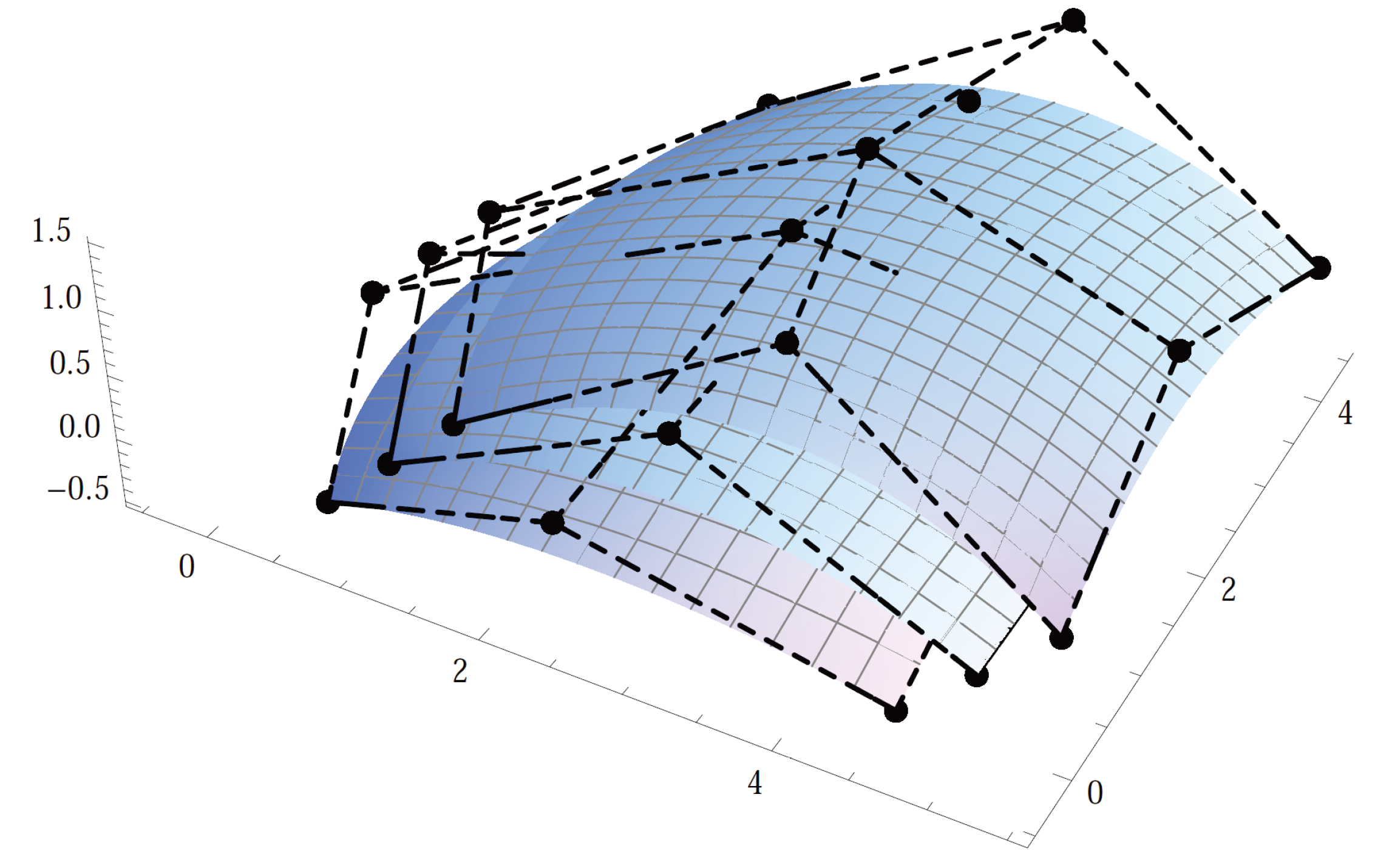
Figure 2.
Fuzzy u-curves.
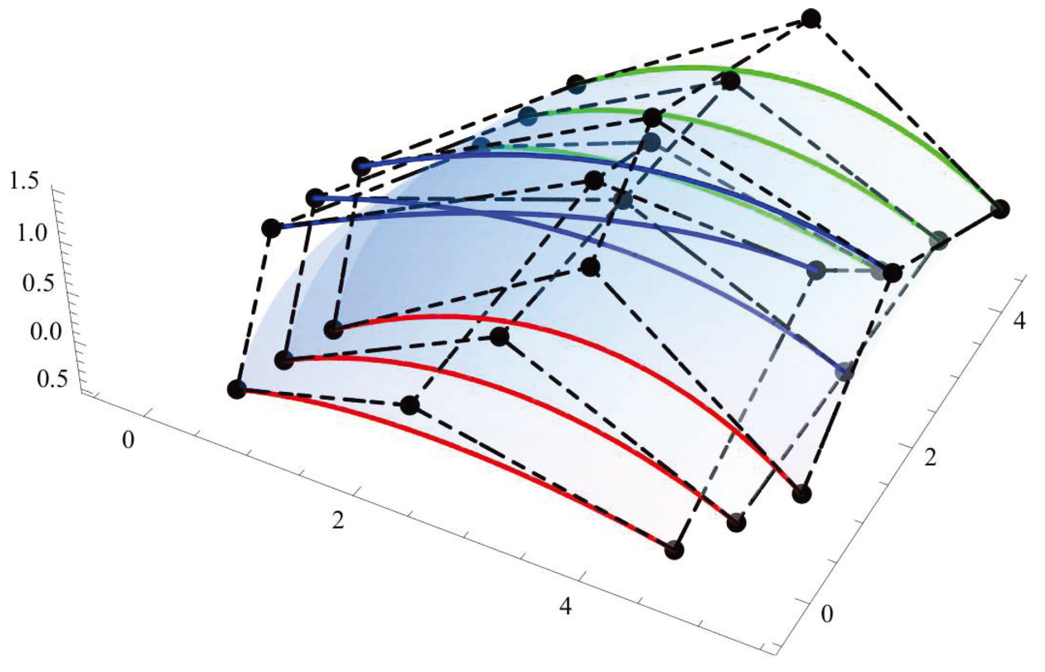
Figure 3.
Fuzzy cubic B.B cuve.

Figure 4.
Fuzzification of Figure 1.
Figure 4.
Fuzzification of Figure 1.

Figure 5.
Defuzzification of Figure 4.
Figure 5.
Defuzzification of Figure 4.

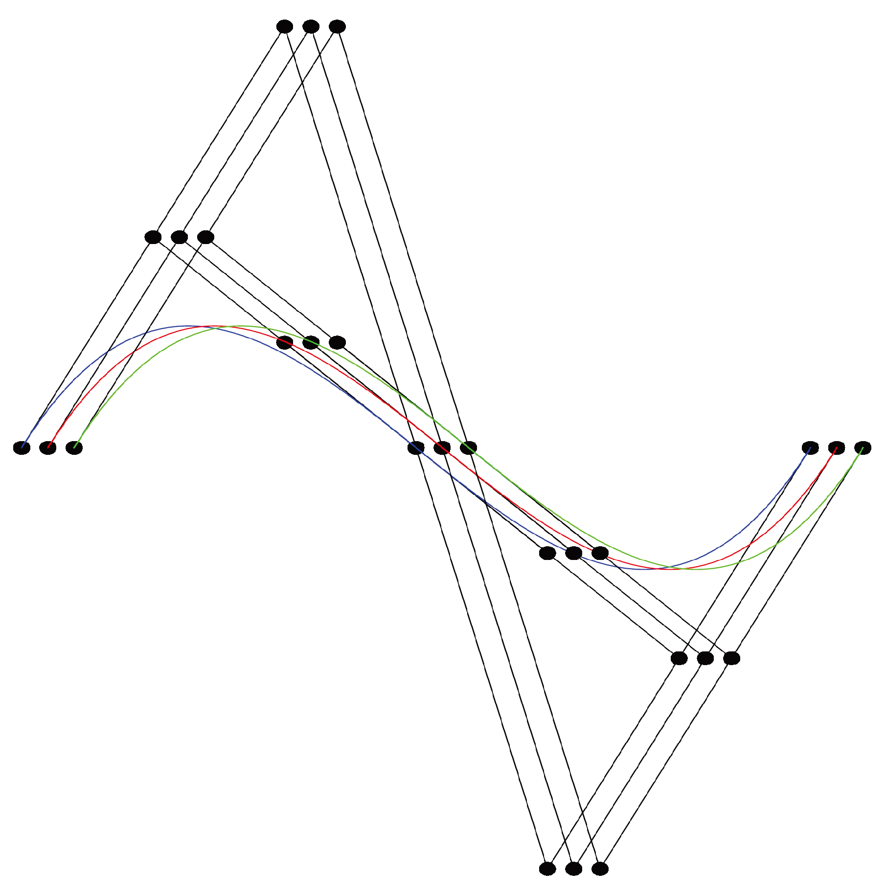
Figure 6.
Fuzzy quadratic B.B curve.

Figure 7.
Fuzzy cubic B.B curve.

Table 1.
Fuzzy control points.
Table 2.
Fuzzy control points.
Table 3.
Fuzzy control points.
| Values on Fuzzy Iso-Parametric Curves for | |
|---|---|
Table 4.
Fuzzy control points.
© 2018 by the authors. Licensee MDPI, Basel, Switzerland. This article is an open access article distributed under the terms and conditions of the Creative Commons Attribution (CC BY) license (http://creativecommons.org/licenses/by/4.0/).
Share and Cite
MDPI and ACS Style
Sarwar, M.; Akram, M. Certain Algorithms for Modeling Uncertain Data Using Fuzzy Tensor Product Bézier Surfaces. Mathematics 2018, 6, 42. https://doi.org/10.3390/math6030042
AMA Style
Sarwar M, Akram M. Certain Algorithms for Modeling Uncertain Data Using Fuzzy Tensor Product Bézier Surfaces. Mathematics. 2018; 6(3):42. https://doi.org/10.3390/math6030042
Chicago/Turabian StyleSarwar, Musavarah, and Muhammad Akram. 2018. "Certain Algorithms for Modeling Uncertain Data Using Fuzzy Tensor Product Bézier Surfaces" Mathematics 6, no. 3: 42. https://doi.org/10.3390/math6030042
Note that from the first issue of 2016, this journal uses article numbers instead of page numbers. See further details here.