g-Convex Weight Sequences


Department of Computer Science and Information Technology, La Trobe University, Bundoora, VIC 3086, Australia
Mathematics 2018, 6(4), 54; https://doi.org/10.3390/math6040054
Submission received: 5 March 2018
/
Revised: 31 March 2018
/
Accepted: 1 April 2018
/
Published: 5 April 2018
Abstract
:In this paper, we introduce the notion of g-convex weight sequence (gcws) for connected graphs based on the concept of g-convexity and g-weight. g-weight is a natural generalization of the notion of branch weight for trees. We investigate the various questions of realization of an integer sequence as a g-convex weight sequence for trees and some special classes of graphs such as complete graphs, windmill and degenerate windmill graphs and wheels.
1. Introduction
Graph theory is a branch of Discrete mathematics that has applications in several different areas such as anthropology, architecture, biology, chemistry, computer science, economics, psychology, telecommunication networks and so on [1]. Graphs are used to model several discrete real-life problems. Among them, finding a central structure is one of the most important applications of graph theory in other disciplines. The problem of finding a central structure is studied extensively in graph theory under facility location problem. The centrality can be defined in several ways. One of them is using the eccentricity of vertices. The other well studied centrality is using graph convexities. Several types of convexities in graphs have been studied in the literature modeled on similar concepts in topology. One of them, called the g-convexity, has been studied by several authors. See, for example, Feldman-Hogassen [2], Mulder [3] and Nieminen [4]. In [5], Prakash constituted a first approach to a systematic study on the size of convex sets in graphs. In a later paper [6], the author demonstrated an application of g-convexity in mobile ad hoc networks. Apart from this, convex sets are also used for measuring dissimilarities and dynamic search in graphs.
In this paper, we introduce the notion of g-convex weight sequences (gcws for short) for graphs. We investigate the various questions of realization of gcws for trees and some special classes of graphs. We believe that the general realization question is an NP-hard (non-deterministic polynomial-time hard)problem. We address this conjecture in our future paper.
We now present some of the graph-theoretic definitions used throughout this paper. Standard graph theoretic terms not defined here can be found in Bondy and Murty [7]. A graph G = (V, E) consists of a finite set V of vertices and a set E of edges, where E is a subset of the set of two-element (unordered) subsets of V. In this paper, we consider only undirected connected finite simple graphs.
The g-convexity and the g-centroid are defined as follows:
Definition 1.
A set is geodetic convex (g-convex for short) if every , all vertices on any shortest path (also called a geodesic path) belong to S.
Definition 2.
Let G = (V, E) be any connected graph. For , we define the g-weight = max {: S is a g-convex set of G not containing v}. Let = min {: }. Then, is called the g-centroidal number of G. The vertices v for which = are called the g-centroidal vertices. The g-centroid is the set of all g-centroidal vertices.
A positive sequence W = {, , ⋯, } of integers is said to be a g-convex weight sequence (gcws for short) if there exists a graph G whose vertices have weights = , . Then, we say G realizes W. When equal weights appear in the sequence, we use the power notation {,, ⋯, }, where s are the multiplicities of and ’s are arranged in the increasing order of magnitude. Clearly, = and = .
Let be a class of graphs. A gcws is said to be potential for if at least one realization of the gcws is a graph in and it is said to be forcible for if every realization of it is a graph in .
For , we denote by = , any maximum g-convex set of G, not containing v.
If the context is clear, we use the term convexity instead of g-convexity.
We now define some graph-theoretic terms, which we will frequently use in the sequel.
Definition 3.
Let G be a connected graph and . The distance between x and y, denoted as is defined as the number of edges in a shortest path connecting x and y in G
In a connected graph G, let , and let = {x : }. We say y is a successor of x with respect to u if and . x is also called a parent or a predecessor of y. Now, consider the successor relation with respect to u on G. Let . We say y is a decendant of some if and there exists an geodesic of length in G. In this case, x is also called an ancestor of y.
By the neighbourhood structure of a graph with respect to a vertex u, we mean the predecessor–successor relation on the vertex set of G defined with respect to u.
The rest of the paper is organized as follows: in Section 2, we address the problem of an integer sequence W to be a gcws for trees. We also provide characterization of an integer sequence to be a gcws for special classes of trees such as stars, caterpillars and spiders. Section 3 deals with the gcws for complete graphs, wheels, windmill and degenerate windmill graphs. We then conclude our paper by presenting a conjecture.
2. Convex Weight Sequences for Trees
In this section, we present a realization for a sequence to be a gcws for a tree. We also characterize gcws for special classes of trees, such as paths, stars, caterpillars and spiders.
A tree is a connected acyclic graph. Vertices of degree one in a tree T are called the leaves of T. Let . Consider the neighbourhood structure of T with respect to u. A vertex is said to be a k-leaf if k is the distance of x from the farthest leaf of T, which is a descendant of x. From the definition of k-leaves, it follows that 0-leaves are the same as leaves.
Let T be a tree and . Then, by the branches at u, we mean the components of . The branch weight of u, denoted by , is the size of the maximum component of . The branch weight centroid of T is the collection of vertices with minimum branch weight. Since every component of is a g-convex set of T, not containing u, it follows that the g-centroid and the branch weight centroid for a tree are the same. Thus, g-centroid is also regarded as the generalization of the branch weight centroid for trees.
The following proposition is applicable to any general graph.
Proposition 1.
Let G = (V, E) be any connected graph and . If , then for any , .
Proof.
Let G be a connected graph and . Let , and be any g-convex set realizing the weight of v. If , then, by the definition of , —a contradiction. Thus, ☐
As an immediate corollary, we have the following result:
Corollary 1.
For any , .
We now present some results concerning the gcws for trees that are used in the sequel.
The proof of the following lemma is immediate from the definition of a leaf vertex.
Lemma 1.
Let T be a tree on n vertices and . = () if and only if u is a leaf of T.
The following proposition establishes a relation between the neighbourhood structure of a tree T at an arbitrary vertex u, and the component of T that realizes the weight of every vertex v of T, such that .
Proposition 1.
Let T be a tree and such that . Consider the neighbourhood structure of T with respect to u. Let be the set of all descendants of v with respect to u, including v. Then, = .
Proof.
Let T be a tree and such that . Consider the neighbourhood structure of T with respect to u. Let , , ⋯, be the branches at v. Without loss of generality, assume that . If possible, let for some . Since , . Thus, , a contradiction. Thus, = = . ☐
The above proposition is true for a centroidal vertex of a tree. Thus, we have the following corollary.
Corollary 2.
Let T be a tree and . Consider the neighbourhood structure of T with respect to u. Let be any arbitrary vertex of T. Let be the set of all descendants of v with respect to u, including v. Then, = .
The following is a well-known theorem of Jordan [1].
Theorem 1.
Let T be a tree. Then, the centroid of T consists of either a single vertex or a pair of adjacent vertices.
The following lemma is true for any arbitrary connected graph G.
Lemma 2.
For any vertex v of G, , where is the maximum clique size of G.
The proof follows from the fact that a clique is a g-convex set of any graph G.
The next proposition establishes a necessary and sufficient condition for a vertex to be a candidate for a g-centroidal vertex in a tree.
Proposition 2.
Let T be a tree and . Then, if and only if every branch at u have less than or equal to vertices.
Proof.
Let and , , ⋯, be the branches at u. If possible, let for some i. We split our discussion into two cases depending on whether n is odd or even.
Let n = and . Since , the i is unique. That is, there is exactly one i such that .
Now, = max { : } = . Let = . Consider the branches of . One branch is and the other branches are , , ⋯, that are subtrees of . It is easy to see that and . Thus, . This is a contradiction, as ; proving the claim in this case.
The proof of the case when n is even is similar to the above.
To prove the converse, let be any arbitrary vertex of T and , , ⋯, be the branches at u such that , . Then, = max {: } . Let v be any arbitrary vertex of T. Without loss of generality, assume that . Since , . As , . Since v is an arbitrary vertex of T, it follows that ☐
The following proposition establishes the connection between the least two weights of a tree and the number of vertices in the tree.
Proposition 3.
Let T be a tree with gcws W = (, , ⋯, ). Then,
- 1.
- 2.
Proof.
The proof for (1) follows from Proposition 2. (2) Let u be a vertex of T with weight . Let be the branches at u. Without loss of generality, assume that = and = . Consider the neighbourhood structure of T with respect to u. From Proposition 1, = = . We now show that is the second least weighted vertex of T. Let v () be any arbitrary vertex belong to . Then, v is a decendant of and from Proposition 1, = . Since is a proper subset of , = = . Let for any . As , = . This establishes that = and thus = n. ☐
As an immediate corollary to (2), we have the following results:
Corollary 3.
A tree T is bicentroidal, then it has even number of vertices.
Proof.
Since T is bicentroidal, = . Thus, = n. Since is an integer, this equation has a solution only when n is even ☐
For any tree T, we can make the following observations:
- Every non-centroidal vertex has exactly one component realizing its weight.
- If a vertex u has more than one component realizing its weight, then T is uni-centroidal and = {u}.
- If T is bi-centroidal, then every vertex of T has exactly one component realizing its weight.
We define a class of graphs called generalized trees as follows: A connected graph G is a generalized tree if the following two properties are satisfied:
- Every non-centroidal vertex of G has exactly one g-convex set realizing its weight.
- If a vertex u has more than one g-convex set realizing its weight, then G is uni-centroidal and = {u}.
It is easy to see that trees and complete graphs belong to the class of generalized trees. It will be an interesting open question to characterize all graphs that belong to this class and study their properties.
2.1. gcws for Paths
In this subsection, we present a sequence that has potential for a path.
The sequence {m, , , ⋯, } has potential for a path on vertices.
The sequence {, , , ⋯, } has potential for a path on vertices.
Remark 1.
If W is a gcws for a path, then, for every integer i, , there are exactly two vertices having weight i. Thus, every number between and is represented in the weight sequence.
2.2. gcws for Star Graphs
In this subsection, we characterize the gcws for stars. A star on n vertices is the complete bipartite graph . The vertices of degree (or the leaves) is the crown of the star.
Proposition 4.
The gcws of a connected graph is {1, } if and only if it is a star.
Proof.
Consider the weight sequence W = {1,}. This is a gcws, since realizes it. We now show that this is the only graph realizing W. Let G be any graph realizing W. Let u be the vertex of G with weight 1. Let be the maximum clique size of G. Then, by Lemma 2, for every vertex v of G, . This holds for u also and hence . If is any edge of , then = 2, a contradiction. Thus, is an independent set. Since G is connected, u is adjacent to every vertex of G and hence G is . ☐
Remark 2.
In the above proof, we have not used the fact that except u, all the other vertices of G have weight (). The assumption that G has a vertex of weight 1 forces that all the other vertices must have weight ().
2.3. gcws for Caterpillars
In this subsection, we discuss the gcws for caterpillars.
A tree is a caterpillar if the deletion of all its leaves produces a path. This path is called the basic path of the caterpillar. The vertices that belong to the basic path are called basic vertices of the caterpillar.
Proposition 5.
Let W = {, , ⋯, , } with and be a potential gcws for a caterpillar. Then, for every i, .
Proof.
Let T be a caterpillar realizing the given weight sequence W. At the outset, it is clear that vertices with weight less than are the basic vertices of T.
From the well-known Jordan’s theorem [1], the branch weight centroid of a tree is either a single vertex or a pair of adjacent vertices. Thus, .
Next we show that , for . On the contrary, assume that . Let ,, be any three vertices of T with weight . Without loss of generality, assume that lies between and in the basic path (as ’s are basic vertices, the basic path contains ,,). Now, consider . If , then { is a g-convex set not containing of cardinality —a contradiction. Hence, and similarly belongs to . Since the geodesic contains , is a g-convex set, it follows that . This is a contradiction. This proves that for . ☐
Remark 3.
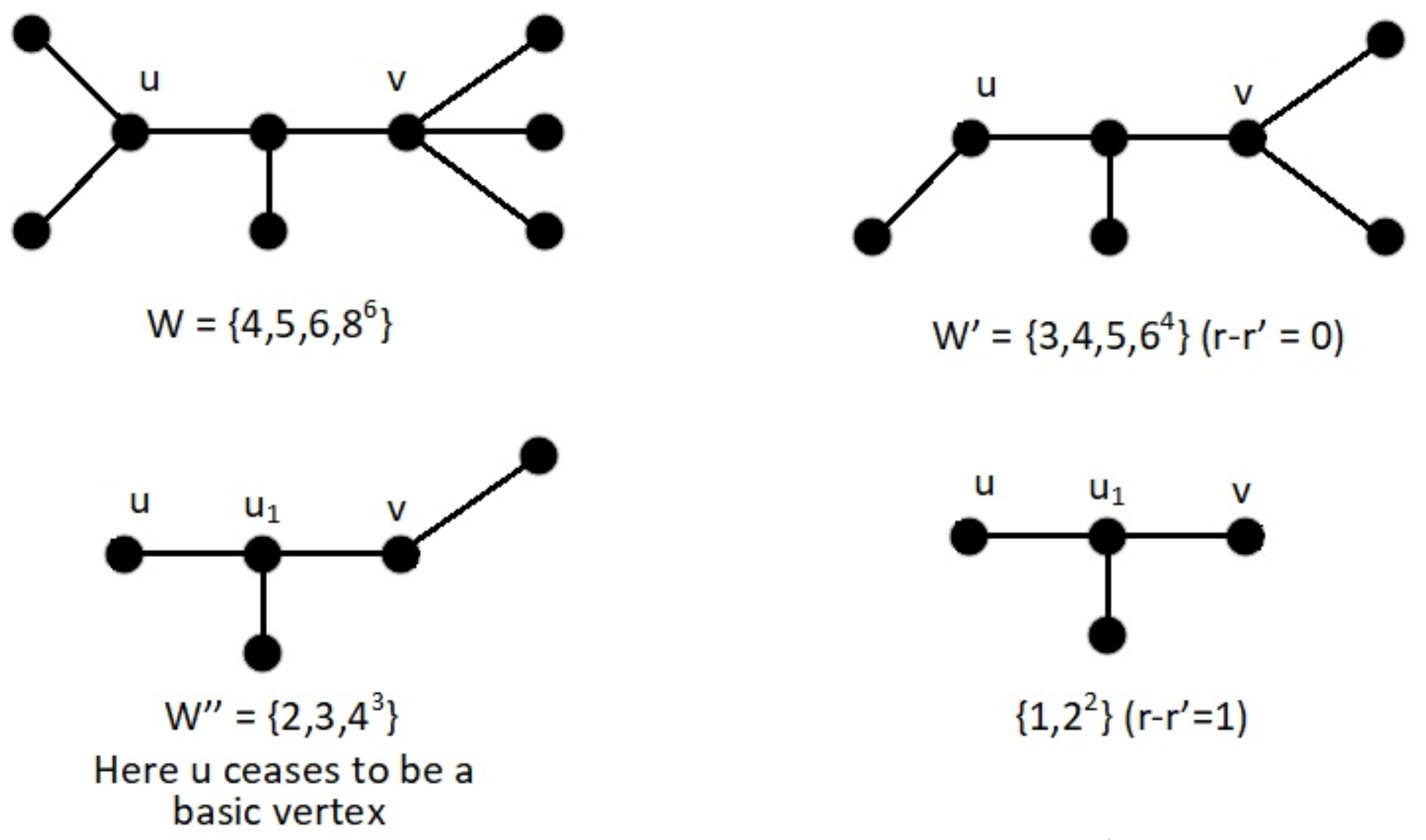
Stars are special types of caterpillars having exactly one basic vertex. We call them as trivial caterpillars. Any caterpillar can be constructed either from a trivial, or from a non-trivial caterpillar by adding two leaves. We capture this property in the following proposition.
Proposition 6.
Let W be the sequence defined in Proposition 5. Then, W is potential gcws for a non-trivial caterpillar if and only if = {, , ⋯, , } is a potential gcws for a caterpillar.
Proof.
Let W as given be the gcws of a caterpillar T. Then, ,, ⋯, are the weights of the basic vertices. Let be the end vertices of the basic path. Since T is a non-trivial caterpillar, such u and v will exist. Then, at least one leaf vertex is attached to u and one to v. Removing one leaf attached to u and one attached with v, the resulting tree is again a caterpillar. It is not difficult to see that the gcws of is . ☐
If the weight of either u or v is , then they cease to be a basic vertex in . Thus, proving the converse is not straightforward.
Conversely, let be a caterpillar realizing . Let be the number of integers less than in (i.e., is the number of basic vertices in ) and r be the number of integers less than in W. It is easy to see that . To prove the converse, we add two leaves to the existing caterpillar. Let and be the end vertices of the basic path in . We may add a leaf to each of and , or one leaf to and other leaf to a leaf vertex attached with , or attach one leaf each to leaf vertices attached with and depending upon the value of .
Case 1
Add a leaf each to and to get a caterpillar T.
Case 2
Add a leaf to and a leaf to a leaf vertex attached to to get T.
Case 3 .
In this case, add a leaf each to a leaf vertex attached to as well as to get T.
In all the three cases, we can easily show that the gcws of T is W.
We illustrate this in Figure 2.
The condition that in Proposition 6 cannot be dropped. This fact is illustrated in Figure 3.
2.4. gcws for Spiders
A tree is a spider if it is a nontrivial homeomorph of a star. The image of the crown of the star under this homeomorphism is the head of the spider. By a spider with parameter (), (), we mean the spider has “legs” on vertices; that is, paths of vertices are joined at the head. We define p =
Paths are special cases of spiders having exactly two legs. The following proposition provides a necessary and sufficient condition for the head of a spider to be a centroidal vertex.
If the context is clear, we refer a spider with parameter (), (), simply as a spider.
Proposition 7.
Let T be a spider and be the head of the spider. Then, if and only if .
The proof follows from the Proposition 2 and the fact that if , then every branch at u has less than or equal to vertices.
The following lemma establishes a relation between a k-leaf of a spider and its weight.
Lemma 3.
Let T be a spider and u be its head. Let . Consider the neighbourhood structure of T with respect to u. Let be a k-leaf. Then, = .
Proof.
Let be a k-leaf with respect to the neighbourhood structure of u. Then, k is the distance to the farthest leaf of T, which is a descendant of v. Since v belongs to a leg, which is a path, v has exactly k-descendants with respect to u. Thus, = . (recall that is the set of all descendants of v with respect to u, including v.) From Proposition 1, = . Thus, = = . ☐
Let T be a spider, u be its head and . Consider the neighbourhood structure of T with respect to u. We list the gcws of T based on the enumeration of the number of k-leaves.
- (1)
- T has p-number of -leaves; . Thus, W has terms { , , ⋯, }.
- (2)
- T has number of -leaves; . Thus, W has terms { , , ⋯, }.
- (3)
- T has number of -leaves; . Thus, W has terms { , , ⋯, }.⋮
- ()
- T has () number of -leaves; . Thus, W has terms { , , ⋯, }.Finally, = .
Thus, the gcws of T is { , , , ⋯, , ⋯, }, where = {: }.
We now discuss the gcws for spiders when . Since , from Proposition 7, , and thus . Let P be the leg on vertices. Depending on whether n is odd or even, T will either be unicentroidal or bicentroidal. Let be a centroidal vertex. Consider the neighbourhood structure of T with respect to . As before, we enumerate the number of number of k-leaves and thus their corresponding term in the weight sequence. It is easy to see that the number of k-leaves are the same for both the case when and for .
Thus, the gcws of T has the following terms: {, , ⋯, }, where = {: }.
Starting from u, the rest of the vertices in P have the following weights depending on whether n is odd or even:
- n odd:
- (), (), (), (), ⋯, (+1), (), (+1), (+2), ⋯, (), (), (),
- n even:
- (), (), (), (), ⋯, (+1), (), (), (+1), (+2), ⋯, (), (), ().
Remark 4.
The following property can be observed from the gcws of a spider:
- (a)
- If , then gcws has contiguous terms starting from () until ().
- (b)
- If , then gcws has contiguous terms starting from () until ().
The following three results establishes a lower bound for the multiplicity of weights in the gcws of a spider.
Proposition 8.
Let T be a spider and W be its gcws. If the multiplicity of the weight () , then , and .
Proof.
Let T be a spider, which is not a path. Let the multiplicity of the weight () . On the contrary, let . Thus, = 1, and the g-centroid lies on a path on vertices. Consider the neighbourhood structure of T with respect to . Then, has two branches with a one containing the head of the spider u (We call this branch as ) and the other branch is a path (We call this branch as ) on vertices.
Since T is not a path, T has at least three legs. Thus, the degree and hence u has at least two children with respect to the neighbourhood structure of . Among them, at least one child is an () leaf and its weight is () ) = (). There is exactly one () leaf in the branch . Based on Corollary 2, starting from u until along the predecessor path, the weight monotonically decreases from to . This sequence contains only when . This inequality relation is possible only when T is a path. Thus, the multiplicity of is 1, a contradiction. This proves that .
Since -leaf is only possible for vertices that belong to the legs on vertices, the multiplicity of implies that . ☐
As a corollary, we have the following result.
Corollary 4.
Let T be a spider, which is not a path. If the multiplicity of the weight () = 1, then = 1.
The proof follows from the fact that, if , then the head of the spider ; and, in this case, every leg on vertices has an -leaf.
Proposition 9.
Let T be a spider, which is not a path with parameter (, , ⋯, ) and W be its gcws. Then, for no , the multiplicity of () = 1.
Proof.
Irrespective of whether the head of the spider u is a centroidal vertex or not, every leg on vertices with has a -leaf. Since , thus the multiplicity of () ≥ 1. ☐
Given an integer sequence W, we present below an algorithm to construct a spider T for which W is the gcws. Our algorithm is based on Proposition 8, 9 and Corollary 4 and the property of gcws for spiders.
Algorithm for Constructing a Spider from its gcws
Let W be an integer sequence. If there is a spider T for which W is the gcws, the proposed algorithm will extract (, , , , ⋯, , ). If the algorithm terminates without extracting the parameters, then W is not a gcws for a spider. However, W may suntil be a gcws of a graph. However, the proposed algorithm here will check only for a spider.
Algorithm
- Input:
- An integer sequence W in a descending order. Where there are multiple terms, power notation is used.
- Step 1:
- The number of terms in W = n. If W is presented in a power-notation, we count the multiplicities.
- Step 2:
- The largest weight in the sequence should be (1); if it is anything else, the algorithm terminates.
- Step 3:
- Let p be the multiplicity of the weight (1).
- Step 3.1:
- Let be the number of contiguous weights (with unit gap) in the sequence having multiplicity p. Then, = .Since r is unknown, we use Proposition 8, 9 and Corollary 4.
- Step 4:
- Let temp be the multiplicity of ().
- -
- If there is exactly one term left in W and the left over term is , then the algorithm terminates successfully. In this case, the spider has p number of legs on vertices attached with the head.
- -
- If the term () is missing, and there are more terms left in the sequence, then the algorithm terminates without success.
- -
- If temp = 1, then r = 2. In this case, = 1; = ; = . If the gcws of T = (, ) is not W, then W is not a gcws of a spider.
- -
- Let temp . Then, = temp; If , then the algorithm terminates without success. If , then the algorithm moves to the next step in extracting the next parameter.
- Step 5:
- Let be the number of contiguous weights in the sequence with multiplicity (). Then, = .
- Step 6:
- If there is only one more term left, then r = 2; = . If the last term is , then W is a gcws; otherwise, it is not.In a similar fashion, we can continue to extract other terms and decide whether W is a gcws or not.
Based on the above steps, we now present an algorithm to verify whether a given integer sequence W is a gcws or not.
Algorithm:
Preprocessing:
- organize the terms of the sequence in a decending order,
- if there are multiple repetitive terms present in the sequence, use the power notation.
Procedure
begin
n = number of terms in W;
if (the largest weight in W = n-1)
continue
else
(exit with FALSE)
p = multiplicity of (n-1)
= number of contiguous weights in
the sequence with multiplicity p; =
i = 1; = p;
loop {
if (only one term left in the sequence and is equal to )
(exit with TRUE);
= multiplicity of (n - 1 - )
if (n - 1 - ) is missing (exit with FALSE)
if ( = 1) {
r = i +1;
= (p - 1 - );
= 1; = (n-1)-;
if the gcws of the spider (,, ⋯, ) is W
then the algorithm terminates successfully
else exit with FALSE }
if () {
= -
if () {exit with FALSE}
= -
i = i + 1
be the number of contiguous terms in the sequence
with multiplcity
} endif
} end loop
end
We now demonstrate the above algorithm through Example 1.
Example 1.
Let W = (, , , , , 22, 21, 20, 8) be an integer sequence. We test if there is a spider that realizes this sequence.
- Step 1:
- n is the number of terms in W (= 28);
- Step 2:
- p is the multiplicity of 27 (= 6);
- Step 3:
- is the number of contiguous weights in W with multiplicity 6, which is 3; .
- Step 4:
- ; ; = multiplicity of (28-1-3 = 24), which is 3.
- Step 5:
- = = 6-3 = 3;
- Step 6:
- = 2;
- Step 7:
- = number of contiguous weights with multiplicity , which is 2;
- Step 8:
- = 3 + 2 = 5;
- Step 9:
- = multiplicity of ( = 22), which is 1.Since is 1, we write the explite gcws and check;= 3; = 1; = = 2;= () = 28 − 1 − 3 × 3 − 2 × 5 = 8;Check whether the gcws of the spider with (,,) is the same as W; since this is “TRUE”; (,,) realizes W.
Remark 5.
From the above propositions and the example, it can be seen that no two spiders have the same gcws.
2.5. gcws for General Trees
In this subsection, we give a set of necessary conditions for a sequence to be potential for trees. Next, we give a necessary and sufficient condition for the same.
We start with a set of necessary conditions.
Proposition 10.
Let W = {, , ⋯, }, such that be the gcws of a tree, then
- 1.
- 2.
- 3.
- if ,if .
Proof.
(1) This follows from the fact that any tree has at least two leaves and the weight of a leaf is . (2) Let . Delete a leaf from a branch at u and append it to u. Let be the gcws of the new tree . Then, without much effort, we can show that . By repeating the procedure, we end up with , for which .
Proof of (3) is similar to that of (2), except that the removed leaf is appended to another leaf. In this case, we end up with a path on n vertices. ☐
Now, we give a necessary and sufficient condition for an integer sequence to be potential for trees.
Proposition 11.
Let W = {, , ⋯, } , such that with be a sequence of positive integers. The W is potential for trees if and only if the following conditions are satisfied.
The sequence , with , can be partitioned into disjoint subsequences , (for some s) of R such that
- 1.
- and
- 2.
- for .
Proof.
(Necessity)
Let T be a tree realizing W. Let be the vertex of T with weight . Let , , ⋯, be the rest of the vertices of T such that . Consider the neighbourhood structure of T with respect to . For each , let be the set of all of descendants of with respect to including . From Corollary 2, for , . Thus, . But . Therefore, . We now define as follows:
If are the neighbours of , then = (. For , if are the children of , then .
We now show that these s form a partition of R and satisfy the conditions (1) and (2).
By the definition of , .
For , from our construction of , = . Therefore, . Thus, satisfy conditions (2).
We now claim that these s’ partitions R. The elements of ’s are s by construction. No can belong to two different and because has a unique father in T with respect to . By the construction of these s, all s are included in s—hence the claim.
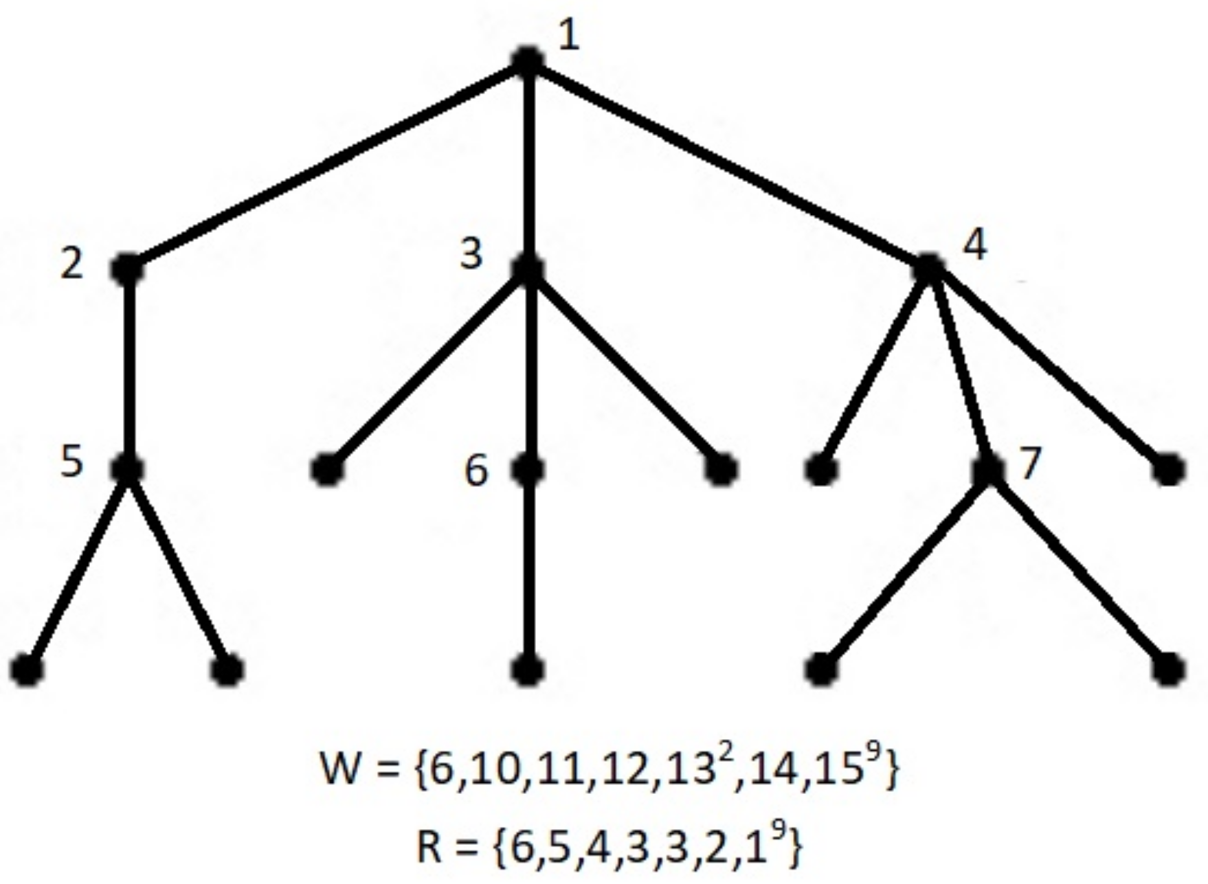
For the sake of clarity, we illustrate this by Figure 6.
Sufficiency.
Let partition R and satisfy conditions (1) and (2). We construct a graph G from these s as follows:
With each , , we associate a vertex and consisting of these s and another vertex . If = (), then = . Join the vertex (i.e., the vertex corresponding to ) with and for , join with . We now show that G is indeed a tree with W as its weight sequence.
Observe that and are adjacent in G if and only if either is in or is in . Thus, we have
= number of parts of ,
= 1 + number of parts of for , and
= 1 for .
Claim 1.
Each is connected to in G and hence G is connected.
Proof of Claim 1.
corresponds to and . If is a part of (), then is joined to . If is a part of for some k, then is joined to . This will stop when , (for, and do not correspond to any element of R). Thus, we have a path from to . This proves the claim.
To show that G is a tree, it is enough to show that . We now show this.
= +
= no. of parts of + (1+no. of parts of ) +
= no. of parts of +
= + = (since ’s partition R and there are
are exactly elements in R, no. of parts of =
We now show that the weight sequence of G is w. ☐
Proof of Claim 2.
Consider . Since , for every i, the only that contains is . Since , . i.e., , as ().
To complete the proof of sufficiency part, consider the neighbourhood structure of G with respect to . consists of all vertices such that and if and only if there exists a vertex in such that . It can easily be proved that each () has exactly descendants with respect to . Thus, by Corollary 2, , . ☐
Remark 6.
The condition that in the above proposition cannot be dropped. This is illustrated by Example 2.
Example 2.
Let W = (3,3,3,4,4). Then, R = (2,2,1,1). Thus, = (2,2), = (1) partitions R, but there is no tree with gcwsW. The proof follows from Jordan’s theorem. Any tree has a maximum of two centroidal vertices; i.e., has a maximum of two vertices with least weight.
Remark 7.
If W is a gcws of a tree, then by taking different set of s satisfying conditions (1) and (2), we get all trees realizing W.
We now show that the only forcible tree sequence is {1,}. To prove this, we need the following lemma.
Lemma 4.
Let T be a tree and . Let be a pair of non-adjacent vertices belonging to the same branch at u. Then, , i.e., the weight of u is same in both graphs T as well as .
Proof of this lemma follows from by a simple observation. However, the weight of the vertices x and y differs in T and . ☐
Now, we have the main proposition
Proposition 12.
The only forcible tree sequence is {1,}.
Proof.
From Proposition 4, {1,} is forcible for stars. Suppose that W is a gcws different from the above, potential for trees. Let T be a tree realizing W. We now show that there exists a graph that is not a tree realizing W.
Let . Consider the neighourhood structure of T with respect to u.
Case 1: There exists a vertex ) with more than one child with respect to u.
Let , be two childeren of v with respect to the neighbourhood structure of u. Since T is a tree, and are not adjacent in T. Let = . We now show that both T and have the same gcws. It is easy to see that = or . We now prove that = . From Corollary 2, = . We also show that is a maximum g-convex set in not containing . Since , from Proposition 1, . Since , no descendant x of belong to , as the geodesic path in passes through . Thus, . Let . Then, it is easy to see that the shortest path between x and y in T and passes through the same vertices. Thus, is a g-convex set in . Thus, we have .
Case 1 exhausts all trees except spiders with the head u being a centrodial vertex.
Case 2: Let T be a spider with the head . Suppose a leaf x is attached to u. Since T is a non-trivial spider, T has a leg L of length . Let and be its child in . Let G = . Then, it is easy to check that gcws(G) = gcws(T).
Suppose that no leaf is attached to u. Let be two legs of T. Let (i = 1, 2) and be a child of in . Let G = . Then, G and T have the same weight sequence. ☐
3. gcws for Some Special Classes of Graphs with Cycles
In this section, we characterize the gcws of some special classes of graphs with cycles, viz. complete graphs, windmill and degenerate windmill graphs and wheels.
A connected graph is complete if and only if every pair of vertices are adjacent.
A graph is a windmill graph is G has exactly one cut vertex and each block of G is a triangle. These triangles are called blades. A graph is a degenerate windmill graph is G is obtained from a windmill graph with at least one blade by attaching at least one pendant edge to its cut vertex.
The wheel is the graph with exactly one cycle of length n and a vertex not in the cycle (called the center of the wheel) adjacent to every vertex in the cycle (these edges are called the spokes for the wheel).
Proposition 13.
A graph is complete if and only if its gcws is {}
Proof.
Obviously, has the weight sequence {}. Conversely, let G be any graph having the gcws {}. Then, for any , and so is a convex set. It can easily be proved that is complete and thus G is complete. ☐
Proposition 14.
The only graph realizing W = {2,} is a windmill or a degenerate windmill graph.
Proof.
Let G be a graph realizing W. Let u be the vertex of G with weight 2.
Claim 1:
u is adjacent with every vertices of G.
If possible, let belong to . Let be the ancestor of v. Then, , as path passes through ; a contradiction as . This proves the claim.
Using the same argument, we can show that has no path on 3-vertices. Since = 2, has at least one edge. Since the weight of every other vertices is n-1, is a union of and . Thus, G is either a windmill or a degenerate windmill graph. ☐
Proposition 15.
The only graph realizing W = {2, } is the graph with at most one cut vertex, whose blocks are either or a wheel with r spokes, .
Proof.
Let G be a graph realizing W. Then, clearly , as .
Case 1: G is a block.
If G is a block on four vertices, then trivially G is . Let . Let u be the vertex of G with weight two. As before, (see Lemma 2).
Claim 1:
Degree of every vertex other than u is three
Suppose v is a vertex of G with . Consider an . By definition, . Let be the other vertex not in (as ). It is easy to see that (otherwise, is complete and hence ). Thus, it follows that contains vertices of . As in previous arguments, these vertices together with v form a complete subgraph of G and thus , a contradiction. Therefore, . We now prove the equality. Clearly, cannot be one, as it would imply . Therefore, we have proved that . To prove , we need the following sub claim.
SubClaim 1:
The eccentricity of u is one, i.e., u is adjacent to all the vertices of G.
First, we show that . If not, let have a descendant z in . Let be a geodesic joining x and z in G. Now, consider . Since , . Hence, . (as geodesic passes through x) Therefore, , a contradiction. Thus, .
It also follows from the above proof that each vertex of has at most one descendant in .
Now, suppose . Let have a descendant y in . If y has no neighbour in and no neighbour other than x in , then . Therefore, y is adjacent to a vertex of or a vertex of N(u). We now discuss the implication of y being adjacent to a vertex in or in (other than x).
Case A: y is adjacent to a vertex in
If is the only geodesic joining x and , then {} is a g-convex set not containing u and hence —a contradiction. Suppose that is another geodesic joining x and . Then, , as x can have at most one descendant in . Since x and are degree saturated (deg = 3), {} is a g-convex set of G. Therefore, ; a contradiction.
Case B: y has an ancestor in
Since , ; otherwise, {x, , y} is a (and thus a g-convex set) not containing u; and hence . Since and G is two-connected, either x or is adjacent to a vertex of (otherwise in , {} are separated from the rest of the vertices). Without loss of generality, assume that is adjacent to of . If is the only geodesic joining and y, as before we get a contradiction. Let be another geodesic joining and y. Then, by our assumption about y, . Clearly, , for then . Consider . Since . Now, cannot contain both and (as an geodesic passes through ). Without loss of generality, assume that . Then, (as a geodesic contains ) and therefore —a contradiction. From cases A and B, we conclude that , i.e., .
We now go back to proving our main claim . If for some v, then it is easy to see that is a clique (as u is adjacent to every vertex of G) and hence , a contradiction. This establishes the claim.
We now show that G is a wheel. Since G is 2-connected, is connected. Since for every vertex v (), is a 2-regular graph. Therefore, is a cycle and hence G is a wheel.
Case 2: G is separable.
Let u be the vertex of G with weight two. First, we show that u is the only cut vertex of G. If not, let v be another cut vertex of G. Since vertices of form a clique (as ), has exactly two components, one with exactly one vertex, say x. Thus, , a contradiction.
In addition, each component of has at least three vertices. For, if a component of has exactly one vertex or a pair of adjacent vertices, then the weight of those vertices is , as their neighbours induce a complete subgraph. As in Case 1, we can prove that each block of G incident with u is either a or a wheel. ☐
4. Conclusions
In this paper, we have presented a necessary and sufficient condition for a sequence to be a gcws for trees. As an immediate generalization, one can try to get such conditions for k-trees, interval graphs and other special classes of graphs such as permutation graphs and circular arc graphs.
Here, we have proved that the gcws are forcible for complete graphs, windmill graphs and degenerate windmill graphs and wheels. One can try to find more such classes.
In this paper, we conjectured that the problem of deciding whether an integer sequence W is gcws or not, is an NP-hard problem. We address this conjecture in our future papers.
We defined a new classes of graphs, which are extensions to trees. We call it as Generalized trees. It will be interesting to classify all graphs that belong to this class and identify the topological properties of graphs that belong to this class.
Conflicts of Interest
The authors declare no conflict of interest.
References
- Bukley, F.; Harary, F. Distance in Graphs; Addison-Wesley: New York, NY, USA, 1991. [Google Scholar]
- Feldman-Hogassen, J. Orders Partiels et Permutoedre. Math. Hum. Sci. 1969, 28, 27–28. [Google Scholar]
- Mulder, H.M. The Interval Function of a Graph; Mathematisch Centrum: Amsterdam, The Netherland, 1980; Volume 132. [Google Scholar]
- Nieminen, J. Centrality, Convexity and Intersections in Graphs. Bull. Math. Soc. Sci. Math. Republ. Soc. Roumania 1984, 28, 337–344. [Google Scholar]
- Veeraraghavan, P. Convexity Studies in Graphs. Ph.D. Thesis, Indian Institute of Technology, Madras, India, 1995. [Google Scholar]
- Veeraraghavan, P. Application of g-Convexity in mobile ad hoc networks. In Proceedings of the 6th IEEE International Conference on Information Technology in Asia, Kuching, Sarawak, Malaysia, 6–9 July 2009. [Google Scholar]
- Bondy, J.A.; Murty, U.S.R. Graph Theory and Its Applications; Elsevier North-Holland: New York, NY, USA, 1976. [Google Scholar]
Figure 1.
Path and a Cyclic graph having the same weight sequence.
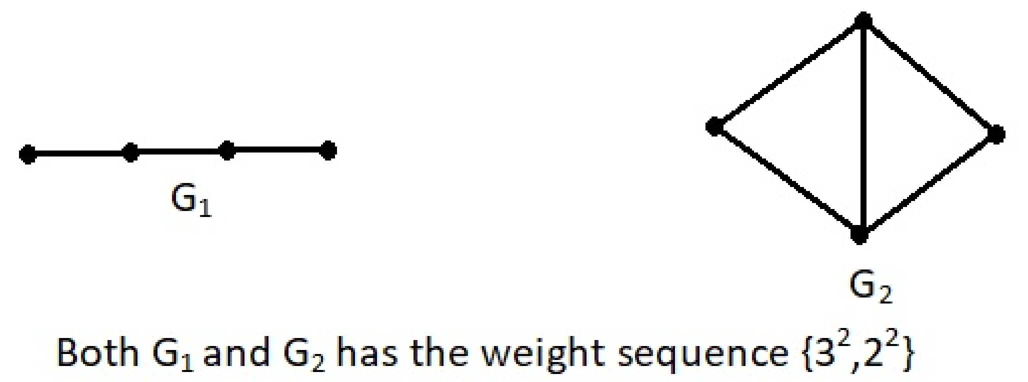
Figure 2.
Example that represents Case 1,2 and 3 of Proposition 6.

Figure 3.
is the only tree with gcws {2, ,}, which is not a caterpillar.

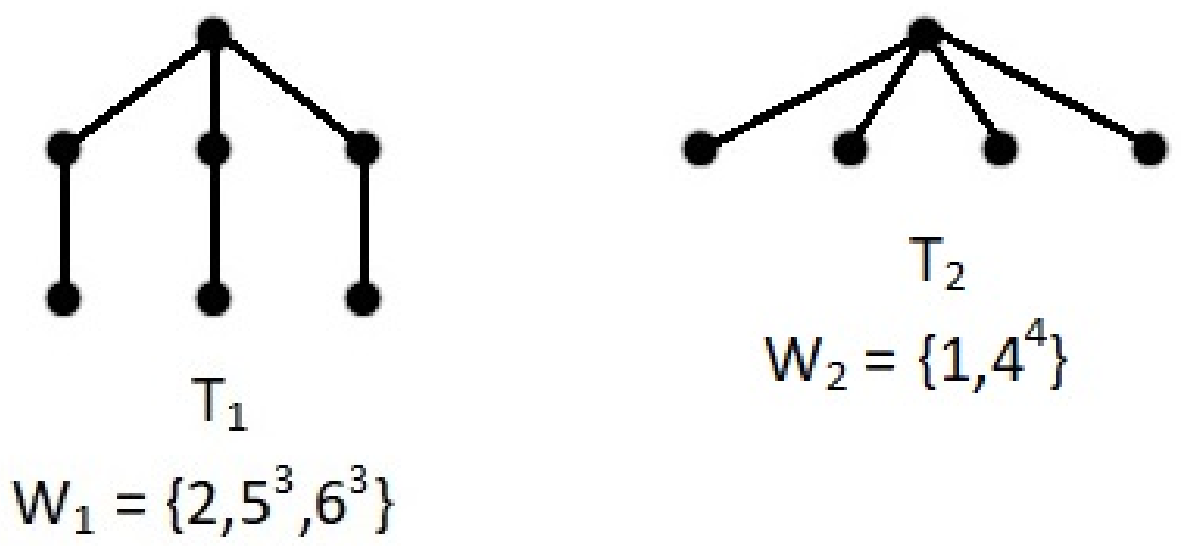
Figure 4.
A non caterpillar and a caterpillar with the same weight sequence.

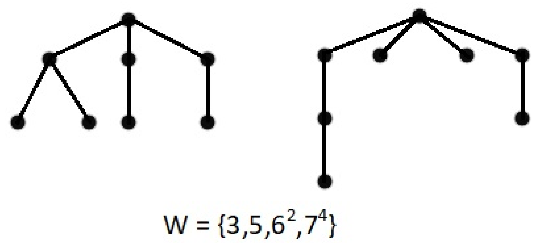
Figure 5.
Two non-isomorphic caterpillars having the same weight sequence.
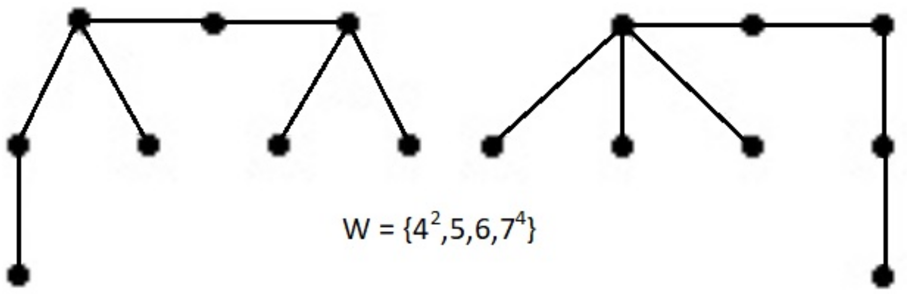
Figure 6.
= (4,5,6), = (3), = (2,1,1), = (1,1,3), = (1,1), = (1), = (1,1).
© 2018 by the author. Licensee MDPI, Basel, Switzerland. This article is an open access article distributed under the terms and conditions of the Creative Commons Attribution (CC BY) license (http://creativecommons.org/licenses/by/4.0/).
Share and Cite
MDPI and ACS Style
Veeraraghavan, P. g-Convex Weight Sequences. Mathematics 2018, 6, 54. https://doi.org/10.3390/math6040054
AMA Style
Veeraraghavan P. g-Convex Weight Sequences. Mathematics. 2018; 6(4):54. https://doi.org/10.3390/math6040054
Chicago/Turabian StyleVeeraraghavan, Prakash. 2018. "g-Convex Weight Sequences" Mathematics 6, no. 4: 54. https://doi.org/10.3390/math6040054
Note that from the first issue of 2016, this journal uses article numbers instead of page numbers. See further details here.