The Emergence of Fuzzy Sets in the Decade of the Perceptron—Lotfi A. Zadeh’s and Frank Rosenblatt’s Research Work on Pattern Classification

The Research Institute for the History of Science and Technology, Deutsches Museum, 80538 Munich, Germany
Mathematics 2018, 6(7), 110; https://doi.org/10.3390/math6070110
Submission received: 25 May 2018
/
Revised: 16 June 2018
/
Accepted: 19 June 2018
/
Published: 26 June 2018
(This article belongs to the Special Issue Fuzzy Mathematics)
Abstract
:In the 1950s, the mathematically oriented electrical engineer, Lotfi A. Zadeh, investigated system theory, and in the mid-1960s, he established the theory of Fuzzy sets and systems based on the mathematical theorem of linear separability and the pattern classification problem. Contemporaneously, the psychologist, Frank Rosenblatt, developed the theory of the perceptron as a pattern recognition machine based on the starting research in so-called artificial intelligence, and especially in research on artificial neural networks, until the book of Marvin L. Minsky and Seymour Papert disrupted this research program. In the 1980s, the Parallel Distributed Processing research group requickened the artificial neural network technology. In this paper, we present the interwoven historical developments of the two mathematical theories which opened up into fuzzy pattern classification and fuzzy clustering.
1. Introduction
“Man’s pattern recognition process—that is, his ability to select, classify, and abstract significant information from the sea of sensory information in which he is immersed—is a vital part of his intelligent behavior.”Charles Rosen [1] (p. 38)
In the 1960s, capabilities for classification, discrimination, and recognition of patterns were demands concerning systems deserving of the label “intelligent”. Back then, and from a mathematical point of view, patterns were sets of points in a mathematical space; however, by and by, they received the meaning of datasets from the computer science perspective.
Under the concept of a pattern, objects of reality are usually represented by pixels; frequency patterns that represent a linguistic sign or a sound can also be characterized as patterns. “At the lowest level, general pattern recognition reduces to pattern classification, which consists of techniques to separate groups of objects, sounds, odors, events, or properties into classes, based on measurements made on the entities being classified”. This said artificial intelligence (AI) pioneer, Charles Rosen, in the introduction of an article in Science in 1967, he claimed in the summary: “This function, pattern recognition, has become a major focus of research by scientists working in the field of artificial intelligence” [1] (p. 38, 43).
The first AI product that was supposed to solve the classification of patterns, such as handwritten characters, was an artificial neuronal network simulation system named perceptron. Its designer was Frank Rosenblatt, a research psychologist at the Cornell Aeronautical Laboratory in Buffalo, New York.
The historical link between pattern discrimination or classification and fuzzy sets documents a RAND report entitled “Abstraction and Pattern Classification”, written in 1964 by Lotfi A. Zadeh, a Berkeley professor of electrical engineering. In this report, he introduced the concept of fuzzy sets for the first time [2]. (The text was written by Zadeh. However, he was not employed at RAND Corporation; Richard Bellman and Robert Kalaba worked at RAND, and therefore, the report appeared under the authorship and order: Bellman, Kalaba, Zadeh; later, the text appeared in the Journal of Mathematical Analysis and Application [3].)
“Pattern recognition, together with learning” was an essential feature of computers going “Steps Toward Artificial Intelligence” in the 1960s as Marvin Lee Minsky postulated already at the beginning of this decade [4] (p. 8). On the 23rd of June of the same year, after four years of simulation experiments, Rosenblatt and his team of engineers and psychologists at the Cornell Aeronautical Laboratory demonstrated to the public their experimental pattern recognition machine, the “Mark I perceptron”.
Another historical link connects pattern recognition or classification with the concept of linear separability when Minsky and Seymour Papert showed in their book, “Perceptrons: an introduction to computational geometry” published in 1969, that Rosenblatt’s perceptron was only capable of learning linearly separable patterns. Turned to logics, this means that a single-layer perceptron cannot learn the logical connective XOR of the propositional logic.
In addition, a historical link combines Zadeh’s research work on optimal systems and the mathematical concept of linear separability, which is important to understand the development from system theory to fuzzy system theory.
We refer to the years from 1957 to 1969 as the decade of the perceptron. It was amidst these years, and it was owing to the research on pattern recognition during the decade of the perceptron, that fuzzy sets appeared as a new “mathematics of fuzzy or cloudy quantities” [5] (p. 857).
This survey documents the history of Zadeh’s mathematical research work in electrical engineering and computer science in the 1960s. It shows the intertwined system of research in various areas, among them, mathematics, engineering and psychology. Zadeh’s mathematically oriented thinking brought him to fundamental research in logics and statistics, and the wide spectrum of his interests in engineering sciences acquainted him with research on artificial neural networks and natural brains as well.
2. Pattern Separation
Today, algorithms in machine learning and statistics solve the problem of pattern classification, i.e., of separating points in a set. More specifically, and in the case of Euclidean geometry, they determine sets of points to be linearly separable. In the case of only two dimensions in the plane, linear separability of two sets A and B means that there exists at least one line in the plane with all elements of A on one side of the line and all elements of B on the other side.
For n-dimensional Euclidean spaces, this generalizes if the word “line” is replaced by “hyperplane”: A and B are linearly separable if there exists at least one hyperplane with all elements of A on one side of the hyperplane and all elements of B on the other side.
Let us consider the case n = 2 (see Figure 1): Two subsets A ⊆ 2n, B ⊆ 2n are linearly separable if there exist n + 1 = 3 real numbers w1, w2, and for all a = (a1, a2) ∈ A, b = (b1, b2) ∈ B it holds
w1a1 + w2 a2 ≤ w3 ≤ w1 b1 + w2 b2.
The points x = (x1, x2) with w1 x1 + w2 x2 = w3 build the separating line.
In 1936, the Polish mathematician, Meier (Maks) Eidelheit (1910–1943), published an article where he proved the later so-called Eidelheit separation theorem concerning the possibility of separating convex sets in normed vector spaces (or local-convex spaces) by linear functionals [6].
One of the researchers who checked the separation theorem for applications in electrical engineering was Lotfi Aliasker Zadeh. He was born in Baku, Azerbaidjan; he studied electrical engineering at the University of Tehran, Iran, and he graduated with a BSc degree in 1942. The following year, he emigrated to the United States (US) via Cairo, Egypt. He landed in Philadelphia, and then worked for the International Electronic Laboratories in New York. In 1944, he went to Boston to continue his studies at the Massachusetts Institute for Technology (MIT). In 1946, Zadeh was awarded a Master’s of Science degree at MIT, and then he changed to Columbia University in New York, where he earned his Doctor of Philosophy (PhD) degree in 1950 for his thesis in the area of continuous analog systems [7]. After being appointed assistant professor, he was searching for new research topics. Both information theory and digital technology interested him, and he turned his attention to digital systems. Zadeh, in an interview with the author on 8 September 1999, in Zittau, at the margin of the 7th Zittau Fuzzy Colloquium at the University Zittau/Görlitz said he “was very much influenced by Shannon’s talk that he gave in New York in 1946 in which he described his information theory.” Zadeh began delivering lectures on automata theory, and in 1949, he organized and moderated a discussion meeting on digital computers at Columbia University, in which Claude E. Shannon, Edmund Berkeley, and Francis J. Murray took part. It was probably the first public debate on this subject ever, as suggested by Zadeh in an interview with the author on 15 June 2001, University of California, Berkeley.)
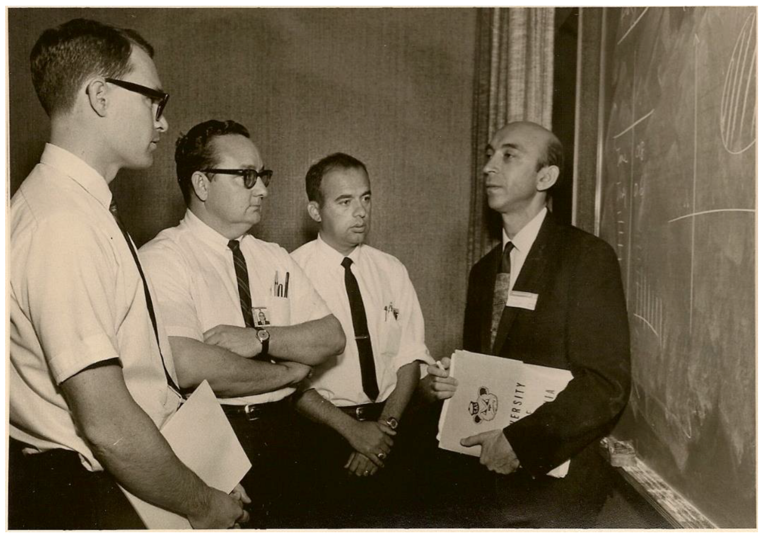
In the second half of the 1950s, Zadeh (Figure 2) became one of the pioneers of system theory, and among his interests, was the problem of evaluating the performance of systems like electrical circuits and networks with respect to their input and their output. His question was whether such systems could be “identified” by experimental means. His thoughts “On the Identification Problem” appeared in the December 1956 edition of “IRE Transactions on Circuit Theory” of the Institute of Radio Engineers [8]. For Zadeh, a system should be identified given (1) a system as a black box B whose input–output relationship is not known a priori, (2) the input space of B, which is the set of all time functions on which the operations with B are defined, and (3) a black box class A that contains B, which is known a priori. Based on the observed response behavior of B for various inputs, an element of A should be determined that is equivalent to B inasmuch as its responses to all time functions in the input space of B are identical to those of B. In a certain sense, one can claim to have “identified” B by means of this known element of A.
Of course, this “system identification” can turn out to be arbitrarily difficult to achieve. Only insofar as information about black box B is available can black box set A be determined. If B has a “normal” initial state in which it returns to the same value after every input, such as the resting state of a linear system, then the problem is not complicated. If this condition is not fulfilled, however, then B’s response behavior depends on a “not normal” initial state, and the attempt to solve the problem gets out of hand very quickly.
All different approaches to solving the problem that was proposed up to that point were of theoretical interest, but they were not very helpful in practice and, on top of that, many of the suggested solutions did not even work when the “black box set” of possible solutions was very limited. In the course of the article, Zadeh only looks at very specific nonlinear systems, which are relatively easy to identify by observation as sinus waves with different amplitudes. The identification problem remained unsolved for Zadeh.
In 1956, Zadeh took a half-year sabbatical at the Institute for Advanced Study (IAS) in Princeton, as disclosed by Zadeh in an interview with the author on 16 June 2001, University of California, Berkeley, that was, for him, the “Mecca for mathematicians”. It inspired him very quickly, and he took back to New York many very positive and lasting impressions. As a “mathematical oriented engineer”—he characterized himself that way in one of my interviews on 26 July 2000, University of California, Berkeley—he now started analyzing concepts in system theory from a mathematical point of view, and one of these concepts was optimality.
In his editorial to the March 1958 issue of the “IRE Transactions on Information Theory”, Zadeh wrote, “Today we tend, perhaps, to make a fetish of optimality. If a system is not ‘best’ in one sense or another, we do not feel satisfied. Indeed, we are not apt to place too much confidence in a system that is, in effect, optimal by definition”. In this editorial, he criticized scalar-valued performance criteria of systems because “when we choose a criterion of performance, we generally disregard a number of important factors. Moreover, we oversimplify the problem by employing a scalar loss function” [9]. Hence, he suggested that vector-valued loss functions might be more suitable in some cases.
3. Optimality and Noninferiority
In September 1963, Zadeh continued the mentioned criticism in a correspondence to the “IEEE Transactions on Automatic Control” of the Institute of Electrical and Electronics Engineers [9]. He emphasized, “one of the most serious weaknesses of the current theories of optimal control is that they are predicated on the assumption that the performance of a system can be measured by a single number”. Therefore, he sketched the usual reasoning with scalar-valued performance criteria of systems as follows: If ∑ is a set of systems and if P(S) is the real-valued performance index of a system S, then a system S0 is called optimal in the ∑ if P(S0) ≥ P(S) for all S ∈ ∑. Thereafter, he criticized that method: “The trouble with this concept of optimality is that, in general, there is more than one consideration that enters into the assessment of performance of S, and in most cases, these considerations cannot be subsumed under a single scalar-valued criterion. In such cases, a system S may be superior to a system S′ in some respects and inferior to S′ in others, and the class of systems ∑ is not completely ordered” [9] (p. 59).
For that reason, Zadeh demanded the distinction between the concepts of “optimality” and “noninferiority”. To define what these concepts mean, he considered the “constraint set” C ⊆ ∑ that is defined by the constraints imposed on system S, and a partial ordering ≥ on ∑ by associating with each system S in ∑ the following three disjoint subsets of ∑:
- (1)
- ∑ > (S), the subset of all systems which are “superior” to S.
- (2)
- ∑ ≤ (S), the subset of all systems, which are inferior or equal (“inferior”) to S.
- (3)
- ∑ ~ (S), the subset of all systems, which are not comparable with S.
That followed Zadeh’s definition of the system’s property of “noninferiority”:
Definition 1.
A system S0 in C is noninferior in C if the intersection of C and ∑> (S0) is empty: C ∩ ∑> (S0) = Ø.
Therefore, there is no system in C, which is better than S0.
The system’s property of optimality he defined, as follows:
Definition 2.
A system S0 in C is optimal in C if C is contained in ∑ ≤ (S0): C ⊆ ∑ ≤ (S).
Therefore, every system in C is inferior to S0 or equal to S0.
These definitions show that an optimal system S0 is necessarily “noninferior”, but not all noninferior systems are optimal.
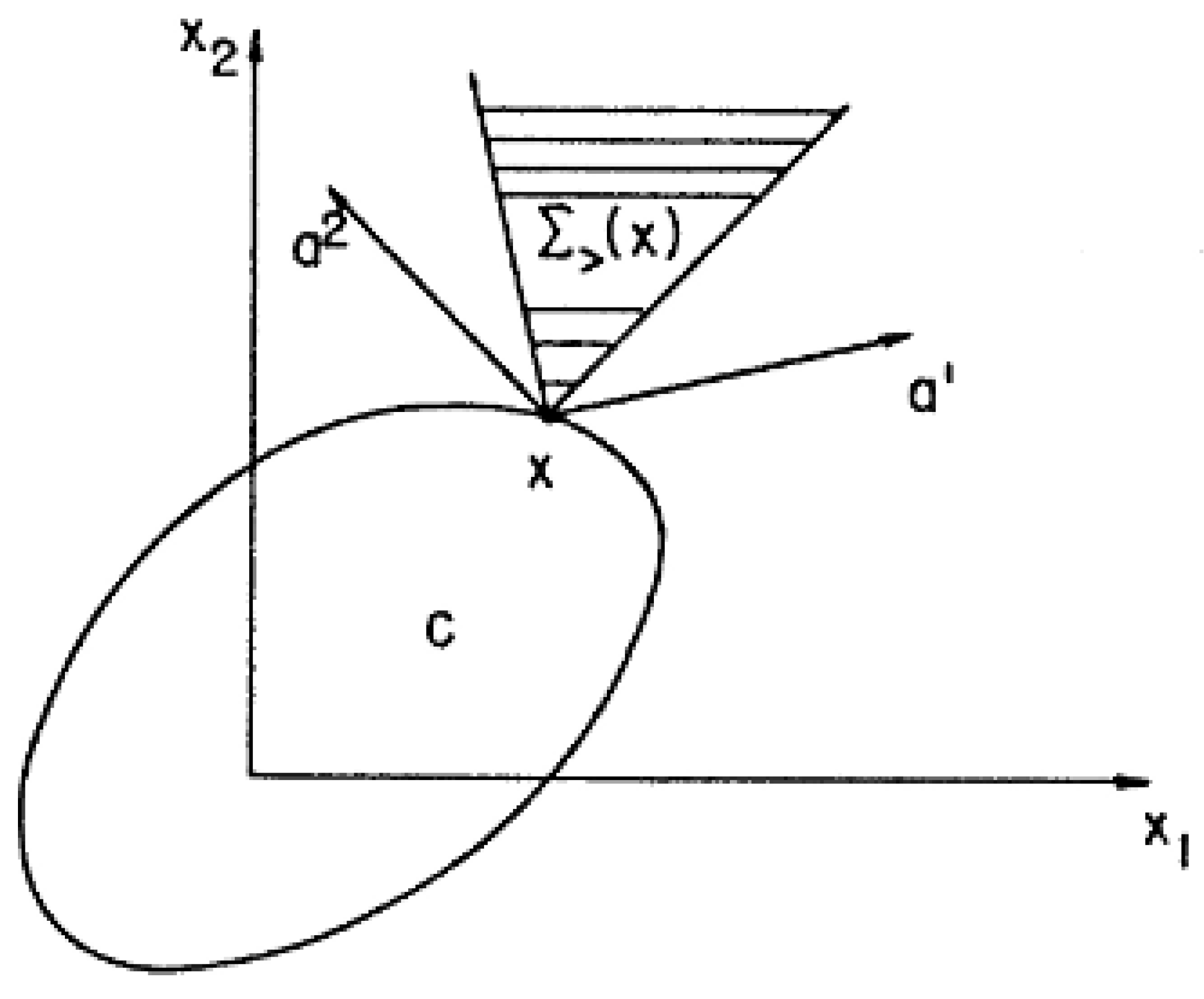
Zadeh considered the partial ordering of the set of systems, ∑, by a vector-valued performance criterion. Let system S be characterized by the vector x = (x1, ..., xn), whose real-valued components represent, say, the values of n adjustable parameters of S, and let C be a subset of n-dimensional Euclidean space Rn. Furthermore, let the performance of S be measured by an m vector p(x) = [p1(x), ..., pm(x)], where pi(x), i = 1, ..., m, is a given real-valued function of x. Then S ≥ S′ if and only if p(x) ≥ p(x′). That is, pi(x) ≥ pi (x′), i = 1, ..., m.
Figure 3 illustrates “the case where ∑> (S) or, equivalently, ∑> (x) is a fixed cone with a vertex at x, and the constraint set C is a closed bounded subset of Rn” [9] (p. 59).
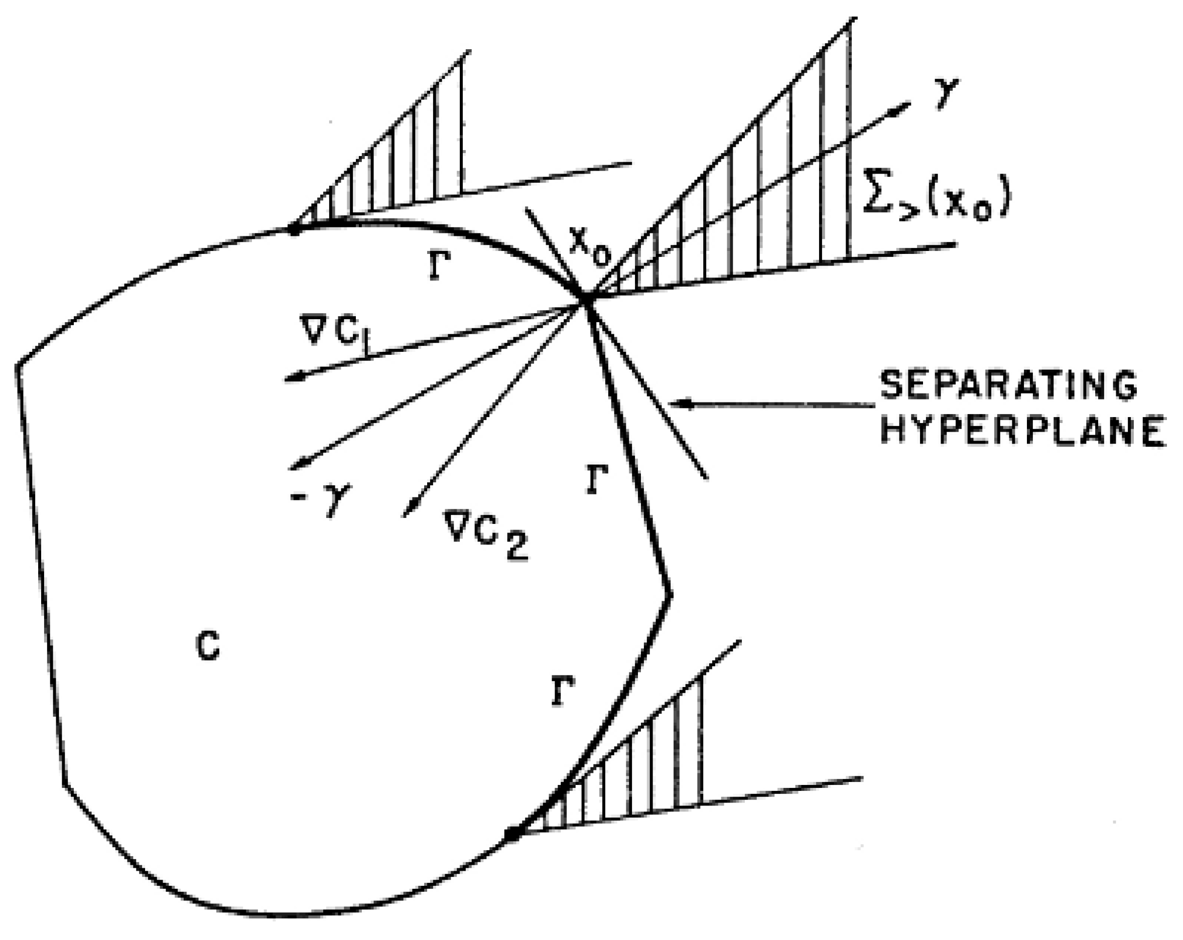
If pi(x) = aiix1 + ... + anxni, where ai = (aii, ..., ani) is the gradient of pi(x), ai = grad pi(x) (a constant vector), then, ∑> (x) is the polar cone of the cone spanned by ai. By definition, noninferior points cannot occur in the interior of the set C. If C is a convex set, then the set of all noninferior points on the boundary of C is the set Γ of all points x0, through which hyperplanes separating the set C and the set ∑> (x0) can be passed. Figure 4 shows the set Γ heavy-lined on the boundary of C.
In this example, ∑> (x0) and C are convex sets, and for convex sets, the separation theorem says that there exists a hyperplane, which separates them.
4. Rosenblatt’s Perceptron
Among other researchers who studied the separability of data points was Frank Rosenblatt, a research psychologist at the Cornell Aeronautical Laboratory in Buffalo, New York. Rosenblatt was born in New Rochelle, New York on 11 July 1928. In 1957, at the Fifteenth International Congress of Psychology held in Brussels, he suggested a “theory of statistical separability” to interpret receiving and recognizing patterns in natural and artificial systems.
In 1943, Warren McCulloch and Walter Pitts published the first model of neurons that was later called “artificial” or “McCulloch–Pitts neuron”. In their article, “A logical calculus of the ideas immanent in nervous activity”, they “realized” the entire logical calculus of propositions by “neuron nets”, and they arrived at the following assumptions [10] (p. 116):
- The activity of the neurons is an “all-or-none” process.
- A certain fixed number of synapses must be excited within the period of latent addition in order to excite a neuron at any time, and this number is independent of previous activity and position on the neuron.
- The only significant delay within the nervous system is synaptic delay.
- The activity of any inhibitory synapse prevents without exception the excitation of the neuron at that time.
The structure of the net does not change with time.
In 1949, based on neurophysiological experiments, the Canadian psychologist, Donald Olding Hebb, proposed the later so-called “Hebb learning rule”, i.e., a time-dependent principle of behavior of nerve cells: “When an axon of cell A is near enough to excite cell B, and repeatedly or persistently takes part in firing it, some growth process or metabolic change takes place in one or both cells so that A’s efficiency, as one of the cells firing B, is increased” [11] (p. 62).
In the same year, the Austrian economist, Friedrich August von Hayek, published “The Sensory Order” [12], in which he outlined general principles of psychology. Especially, he proposed to apply probability theory instead of symbolic logic to model the behavior of neural networks which achieve reliable performance even when they are imperfect by nature as opposed to deterministic machines.
Rosenblatt’s theory was in the tradition of Hebb’s and Hayek’s thoughts. The approach of statistical separability distinguishes his model from former brain models. Rosenblatt “was particularly struck by the fact that all of the mathematically precise, logical models which had been proposed to date were systems in which the phenomenon of distributed memory, or ‘equipotentiality’ which seemed so characteristic of all biological systems, was either totally absent, or present only as a nonessential artefact, due to postulated ‘repetitions’ of an otherwise self-contained functional network, which by itself, would be logically sufficient to perform the functions of memory and recall” [13] (p. iii). Therefore, Rosenblatt chose a “model in terms of probability theory rather than symbolic logic” [14] (p. 388).
In his “Probabilistic Model for Visual Perception”, as his talk was entitled [15], he characterized perception as a classification process, and in his first project report that appeared in the following year, he wrote, “Elements of stimulation which occur most commonly together are assigned to the same classes in a ‘sensory order’. The organization of sensory classes (colors, sounds, textures, etc.) thus comes to reflect the organization of the physical environment from which the sensations originate” ([13], p. 8). To verify his theory, Rosenblatt promised the audience a working electronic model in the near future, and for a start, he presented simulations running on the Weather Bureau’s IBM 704. He fed the computer with “two cards, one with squares marked on the left side and the other with squares on the right side”. The program differentiated between left and right after “reading” through about 50 punched cards. “It then started registering a ‘Q’ for the left squares and ‘O’ for the right squares” [13] (p. 8).
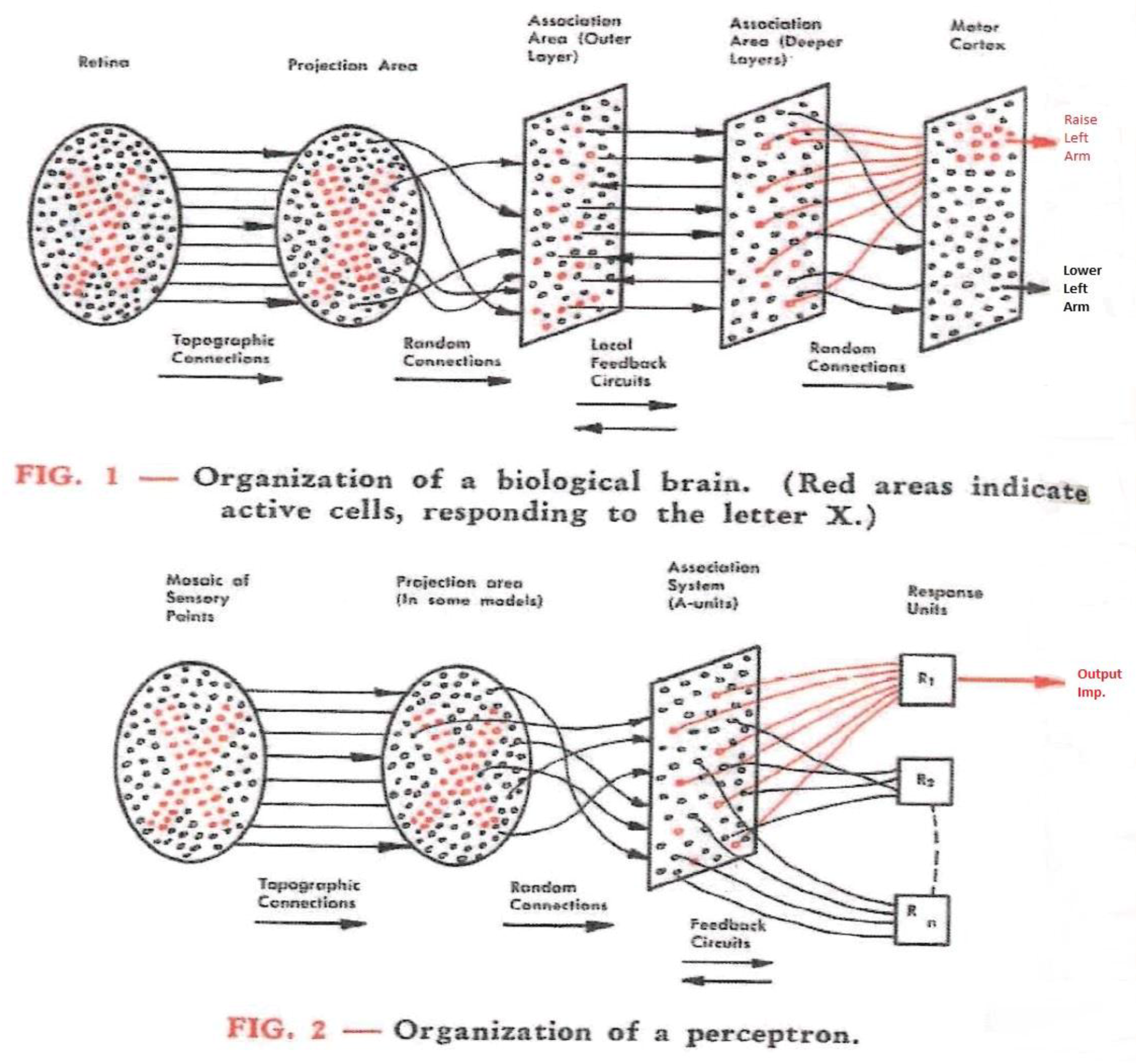
Rosenblatt illustrated the organization of the perceptron via such comparisons with a biological brain, as shown in Figure 5. These illustrations compare the natural brain’s connections from the retina to the visual area with a perceptron that connects each sensory point of the “retina” to one or more randomly selected “A-units” in the association system. The A-units transduce the stimuli, and they increase in value when activated (represented by the red points in Figure 5).
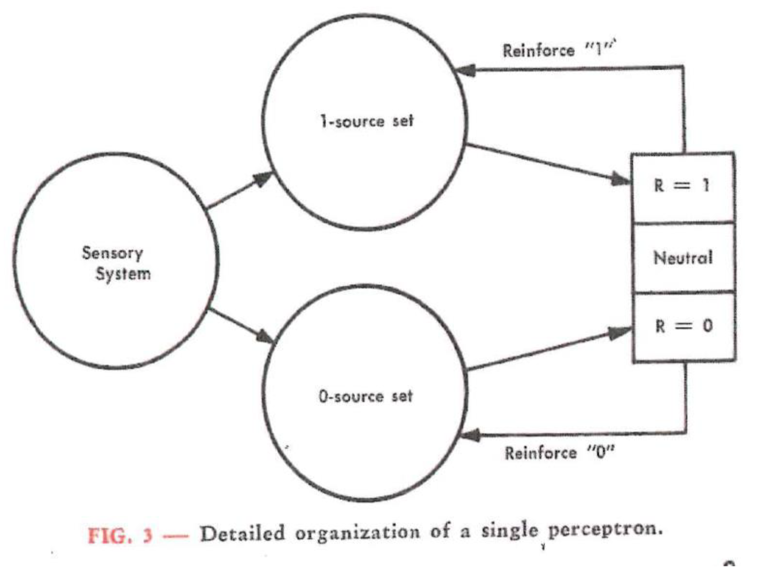
Their responses arrive at “R-units”, which are binary devices (i.e., “on” or “off”, and “neutral” in the absence of any signal because the system will not deliver any output), as Figure 6 shows for a very simple perceptron. The association system has two parts, the upper source set tends to activate the response R = 1, and the lower one tends to activate the response R = 0. From the responses, a feedback to the source set is generated, and these signals multiply the activity rate of the A-unit that receives them. Thus, the activity of the R-units shows the response to stimuli as a square or circle, as presented in the environment. “At the outset, when a perceptron is first exposed to stimuli, the responses which occur will be random, and no meaning can be assigned to them. As time goes on, however, changes occurring in the association systems cause individual responses to become more and more specific to such particular, well-differentiated classes of forms as squares, triangles, clouds, trees, or people” [16] (p. 3).
Rosenblatt attached importance to the following “fundamental feature of the perceptron”: “When an A-unit of the perceptron has been active, there is a persistent after-effect which serves the function of a ‘memory trace’. The assumed characteristic of this memory trace is a simple one: whenever a cell is active, it gains in ‘strength’ so that its output signals (in response to a fixed stimulus) become stronger, or gain in frequency or probability” [16] (p. 3).
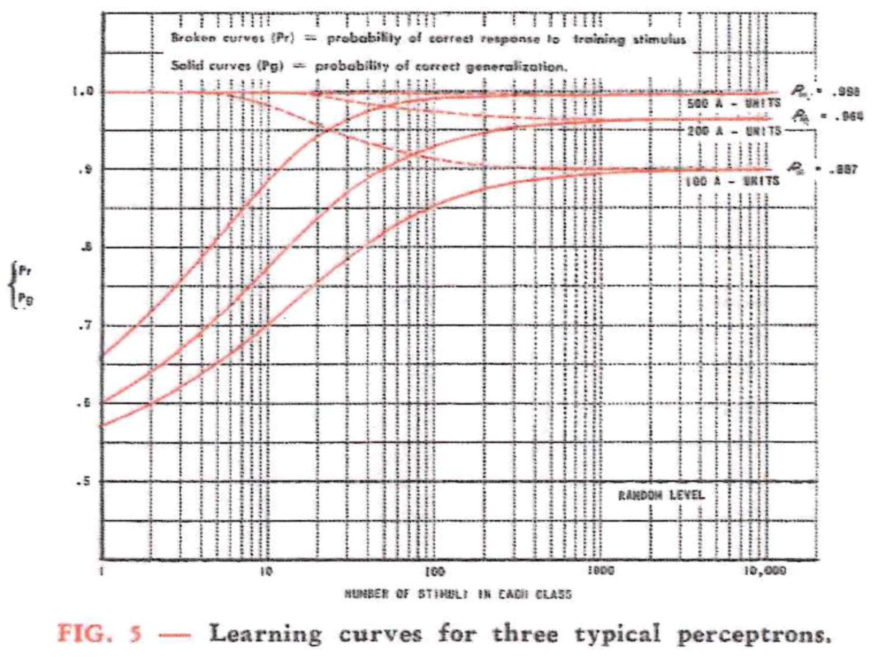
Rosenblatt presented the results of experiments in which a perceptron had to learn to discriminate between a circle and a square with 100, 200, and 500 A-units in each source set of the association system. In Figure 7, the broken curves indicate the probability that the correct response is given when identical stimuli of a test figure were shown during the training period. Rosenblatt called this “the perceptron’s capacity to recollect”. The solid curves show the probability that the appropriate response for any member of the stimulus class picked at random will be given. Rosenblatt called this “the perceptron’s capacity to generalize” [16] (p. 10). Figure 7 shows that both probabilities (capacities) converge in the end to the same limit. “Thus”, concluded Rosenblatt, “in the limit it makes no difference whether the perceptron has seen the particular stimulus before or not; it does equally well in either case” [16] (p. 4).
Clearly, probability theory is necessary to interpret the experimental results gathered with his perceptron simulation system. “As the number of association units in the perceptron is increased, the probabilities of correct performance approach unity”, Rosenblatt claimed, and with reference to Figure 7, he continued, “it is clear that with an amazingly small number of units—in contrast with the human brain’s 1010 nerve cells—the perceptron is capable of highly sophisticated activity [16] (p. 4).
In 1960, on the 23rd of June, a “Perceptron Demonstration”, sponsored by the ONR (Office of Naval Research) and the Directorate of Intelligence and Electronic Warfare, Rome Air Development Center, took place at the Cornell Aeronautical Laboratory. After a period of successful simulation experiments, Rosenblatt and his staff had created the experimental machine Mark I perceptron.
Four hundred photocells formed an imaginary retina in this perceptron—a simulation of the retinal tissue of a biological eye—and over 500 other neuronlike units were linked with these photocells by the principle of contingency, so they could supply them with impulses that came from stimuli in the imaginary retina. The actual perceptron was formed by a third layer of artificial neurons, the processing or response layer. The units in this layer formed a pattern associator.
In this classic perceptron, cells can be differentiated into three layers. Staying with the analogy of biological vision, the “input layer” with its (photo) cells or “stimulus units” (S cells) corresponds to the retinal tissue, and the middle “association layer” consists of so-called association units (A cells), which are wired with permanent but randomly selected weights to S cells via randomly linked contacts. Each A cell can, therefore, receive a determined input from the S layer. In this way, the input pattern of the S layer is distributed to the A layer. The mapping of the input pattern from the S layer onto a pattern in the A layer is considered “pre-processing”. The “output layer”, which actually makes up the perceptron, and which is, thus, also called the “perceptron layer”, contains the pattern-processing response units (R cells), which are linked to the A cells. R and A cells are McCulloch–Pitts neurons, but their synapses are variable and are adapted appropriately according to the Hebb rule. When the sensors detect a pattern, a group of neurons is activated, which prompts another neuron group to classify the pattern, i.e., to determine the pattern set to which said pattern belongs.
A pattern is a point in the x = (x1, x2, ..., xn) n-dimensional vector space, and so, it has n components. Let us consider again just the case n = 2, then a pattern x = (x1, x2) such as this also belongs to one of L “pattern classes”. This membership occurs in each individual use case. The perceptron “learned” these memberships of individual patterns beforehand on the basis of known classification examples it was provided. After an appropriate training phase, it was then “shown” a new pattern, which it placed in the proper classes based on what it already “learned”. For a classification like this, each unit, r, of the perceptron calculated a binary output value, yr, from the input pattern, x, according to the following equation: yr = θ (wr1x1 + wr2x2).
The weightings, wr1 and wr2, were adapted by the unit, r, during the “training phase”, in which the perceptron was given classification examples, i.e., pattern vectors with an indication of their respective pattern class, Cs, such that an output value, yr = 1, occurred only if the input pattern, x, originated in its class, Cr. If an element, r, delivered the incorrect output value, yr, then its coefficients, wr1 and wr2, were modified according to the following formulae:
Δwr1 = εr · (δrs − yr) · x1 and Δwr2 = εr · (δrs − yr) · x2.
In doing so, the postsynaptic activity, yr, used in the Hebb rule is replaced by the difference between the correct output value, δrs, and the actual output value, yr. These mathematical conditions for the perceptron were not difficult. Patterns are represented as vectors, and the similarity and disparity of these patterns can be represented if the vector space is normalized; the dissimilarity of two patterns, v1 and v2, can then be represented as the distance between these vectors, such as in the following definition: d(v1v2) = || v2 − v1 ||.
5. Perceptron Convergence
In 1955, the mathematician Henry David Block came to Cornell where he started in the Department of Mathematics; however, in 1957, he changed to the Department of Theoretical and Applied Mechanics. He collaborated with Rosenblatt, and derived mathematical statements analyzing the perceptron’s behavior. Concerning the convergence theorem, the mathematician, Jim Bezdek, said in my interview: “To begin, I note that Dave Block proved the first Perceptron convergence theorem, I think with Nilsson at Stanford, and maybe Novikoff, in about 1962, you can look this up” [17] (p. 5).
Block published his proof in “a survey of the work to date” in 1962 [18]. Nils John Nilsson was Stanford’s first Kumagai Professor of Engineering in Computer Science, and Albert Boris J. Novikoff earned the PhD from Stanford. In 1958, he became a research mathematician at the Stanford Research Institute (SRI). He presented a convergence proof for perceptrons at the Symposium on Mathematical Theory of Automata at the Polytechnic Institute of Brooklyn (24–26 April 1962) [19]. Other versions of the algorithm were published by the Russian control theorists, Mark Aronovich Aizerman, Emmanuel M. Braverman, and Lev I. Rozonoér, at the Institute of Control Sciences of the Russian Academy of Sciences, Moscow [20,21,22].
In 1965, Nilsson wrote the book “Learning Machines: Foundations of Trainable Pattern-Classifying Systems”, in which he also described in detail the perceptron’s error correction and learning procedure. He also proved that for separable sets, A and B, in the n-dimensional Euclidean space, the relaxation (hill-climbing/gradient) algorithm will converge to a solution in finite iterations.
Judah Ben Rosen, an electrical engineer, who was head of the applied mathematics department in the Shell Development Company (1954–1962) came as a visiting professor to Stanford’s computer science department (1962–1964). In 1963, he wrote a technical report entitled “Pattern Separation by Convex Programming” [23], which he later published as a journal article [24].
Coming from the already mentioned separation theorem, he showed “that the pattern separation problem can be formulated and solved as a convex programming problem, i.e., the minimization of a convex function subject to linear constraints” [24] (p. 123). For the n-dimensional case, he proceeded as follows: A number l of point sets in an n-dimensional Euclidean space is to be separated by an appropriate number of hyperplanes. The mi points in the ith set (where i = 1, ..., l) are denoted by n-dimensional vectors, pij, j = 1, ..., mi. Then, the following matrix describes the points in the ith set:
Pi = pi1, pi2, ..., pimi.
In the simplest case, at which the Rosenblatt perceptron failed, two points, P1 and P2, are to be separated. Rosen provides this definition:
Definition 3.
The point sets, P1 and P2, are linearly separable if their convex hulls do not intersect. (The convex hull of a set is the set of all convex combinations of its points. In other words, given the points pi from P and given λi from R, then the following set is the convex hull of P: conv (P) = λ1·p1 + λ2·p2 + ... + λn·pn.)
An equivalent statement is the following:
“The point sets, P1 and P2, are linearly separable if and only if a hyperplane
H = H(z,α) = {p|p′z = α} exists such that P1 und P2 lie on the opposite sides of H. (p′ refers to the transpose of p.)
The orientation of the hyperplane H is, thus, specified by the n-dimensional unit vector, z, and its distance from the origin is determined by a scalar, α. The linear separation of P1 and P2 was, therefore, equivalent to demonstrating the existence of a solution to the following system of strict inequalities. (Here || || denotes the Euclidean norm, and ei is the mi-dimensional unit vector):
| p1jz > α j = 1, ..., m1 |
| p2jz < α j = 1, ..., m2 || z || = 1, |
| p1jz > α e1 |
| p2jz < α e2 || z || = 1. |
Rosen came to the conclusion “that the pattern separation problem can be formulated and solved as a convex programming problem, i.e., the minimization of a convex subject to linear constraints”. [24] (p. 1) He considered the two linearly separable sets, P1 and P2. The Euclidean distance, δ, between these two sets is then indicated by the maximum value of γ, for which z and α exist such that
| P′1z ≥ (α + ½ γ)e1 |
| P′2z ≤ (α + ½ γ)e2 || z || = 1. |
The task is, therefore, to determine the value of the distance, δ, between the sets, P1 and P2, formulated as the nonlinear programming problem that can find a maximum, γ, for which the above inequalities are true. Rosen was able to reformulate it into a convex quadratic programming problem that has exactly one solution when the points, P1 and P2, are linearly separable. To do so, he introduced a vector, x, and a scalar, β, for which the following applies: , , and . Maximizing γ is, thus, equivalent to minimizing the convex function, :
After introducing the (n + 1)-dimensional vectors, , , and the (n + 1) × mi–matrices, Qi = [qi1, qi2, ..., qimi], Rosen could use the standard form of convex quadratic programming, and formulate the following theorem of linear separability:
Theorem 1.
The point sets, P1 and P2, are linearly separable if and only if the convex quadratic programming problem
has a solution. If P1 and P2 are linearly separable, then the distance, δ, between them is given byand a unique vector,achieves the minimum, σ. The separating hyperplane is given by.
6. Fuzzy Pattern Classification
In the middle of the 1960s, Zadeh also got back to the topics of pattern classification and linear separability of sets. In the summer of 1964, he and Richard E. Bellman, his close friend at the RAND Corporation, planned on doing some research together. Before that, there was the trip to Dayton, Ohio, where he was invited to talk on pattern recognition in the Wright-Patterson Air Force Base. Here, within a short space of time, he developed his little theory of “gradual membership” into an appropriately modified set theory: “Essentially the whole thing, let’s walk this way, it didn’t take me more than two, three, four weeks, it was not long”, Said (Zadeh in an interview with the author on June 19, 2001, UC Berkeley.) When he finally met with Bellman in Santa Monica, he had already worked out the entire theoretical basis for his theory of fuzzy sets: “His immediate reaction was highly encouraging and he has been my strong supporter and a source of inspiration ever since”, said (Zadeh in “Autobiographical Note 1”—an undated two-page typewritten manuscript, written after 1978.)
Zadeh introduced the conceptual framework of the mathematical theory of fuzzy sets in four early papers. Most well-known is the journal article “Fuzzy Sets” [25]; however, in the same year, the conference paper “Fuzzy Sets and Systems” appeared in a proceedings volume [26], in 1966, “Shadows of Fuzzy Sets” was published in Russia [27], and the journal article “Abstraction and Pattern Classification” appeared in print [4]. The latter has three official authors, Bellman, Kalaba, and Zadeh, but it was written by Zadeh; moreover, the text of this article is the same as the text of a RAND memorandum of October 1964 [3]. By the way, preprints of “Fuzzy Sets” and “Shadows of Fuzzy Sets” [28] appeared already as “reports” of the Electronic Research Laboratory, University of California, Berkeley, in 1964 and 1965 ([29], Zadeh 1965c).
Fuzzy sets “do not constitute classes or sets in the usual mathematical sense of these terms”. They are “imprecisely defined ‘classes’”, which “play an important role in human thinking, particularly in the domains of pattern recognition, communication of information, and abstraction”, Zadeh wrote in his seminal paper [25] (p. 338). A “fuzzy set” is “a class in which there may be a continuous infinity of grades of membership, with the grade of membership of an object x in a fuzzy set A represented by a number μA(x) in the interval [0, 1]” [26] (p. 29). He defined fuzzy sets, empty fuzzy sets, equal fuzzy sets, the complement, and the containment of a fuzzy set. He also defined the union and intersection of fuzzy sets as the fuzzy sets that have membership functions that are the maximum or minimum, respectively, of their membership values. He proved that the distributivity laws and De Morgan’s laws are valid for fuzzy sets with these definitions of union and intersection. In addition, he defined other ways of forming combinations of fuzzy sets and relating them to one another, such as, the “algebraic sum”, the “absolute difference”, and the “convex combination” of fuzzy sets.
Concerning pattern classification, Zadeh wrote that these “two basic operations: abstraction and generalization appear under various guises in most of the schemes employed for classifying patterns into a finite number of categories” [3] (p. 1). He completed his argument as follows: “Although abstraction and generalization can be defined in terms of operations on sets of patterns, a more natural as well as more general framework for dealing with these concepts can be constructed around the notion of a ‘fuzzy’ set—a notion which extends the concept of membership in a set to situations in which there are many, possibly a continuum of, grades of membership” [3] (p. 1).
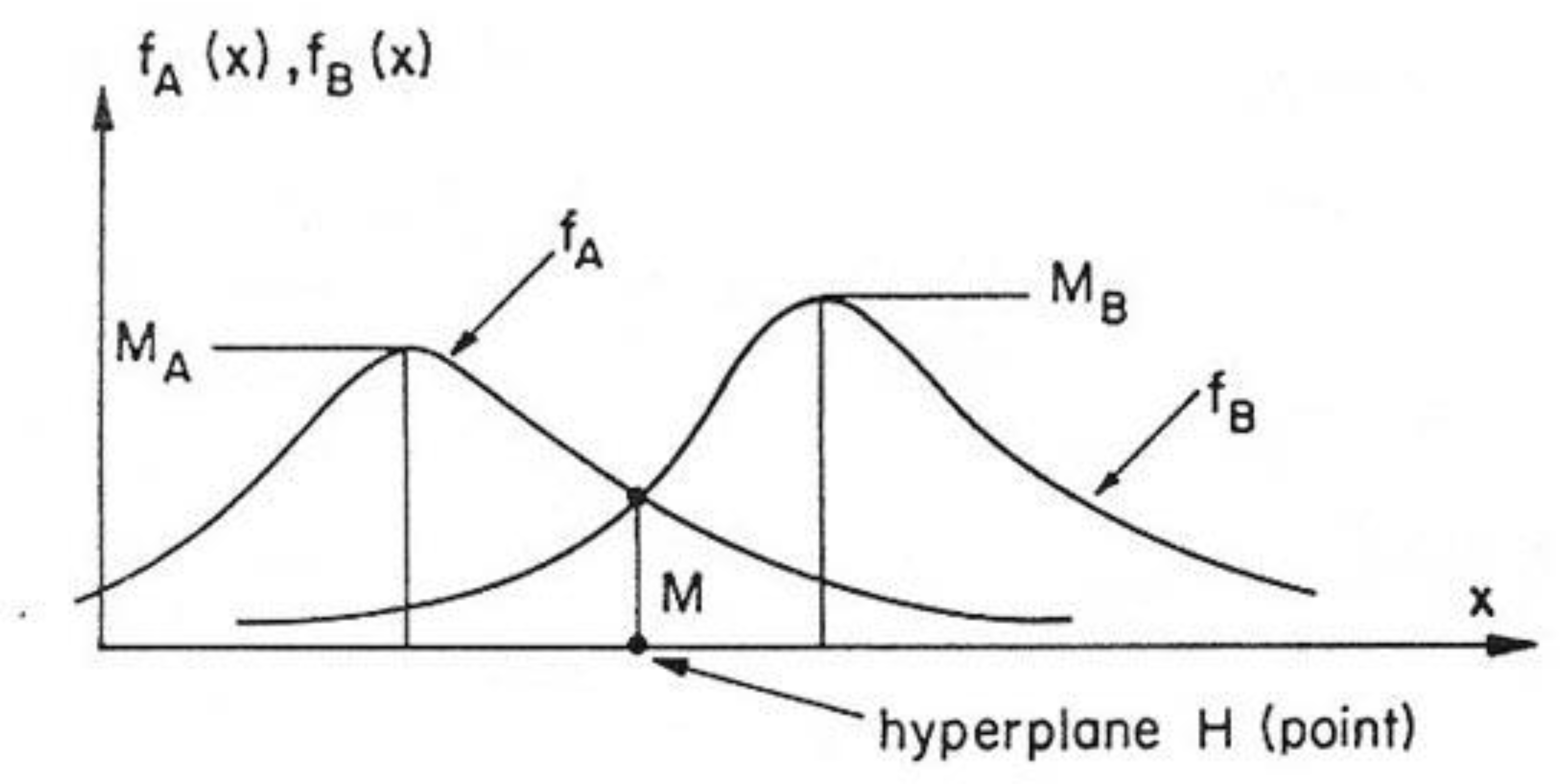
After a discussion of two definitions of “convexity” for fuzzy sets and the definition of “bounded” fuzzy sets, he defined “strictly” and “strongly convex” fuzzy sets. Finally, he proved the separation theorem for bounded convex fuzzy sets, which was relevant to the solution of the problem of pattern discrimination and classification that he perhaps presented at the Wright-Patterson Air Force Base (neither a manuscript nor any other sources exist; Zadeh did not want to either confirm or rule out this detail in the interviews with the author). At any rate, in his first text on fuzzy sets, he claimed that the concepts and ideas of fuzzy sets “have a bearing on the problem of pattern classification” [2] or [3] (p. 1). “For example, suppose that we are concerned with devising a test for differentiating between handwritten letters, O and D. One approach to this problem would be to give a set of handwritten letters, and to indicate their grades of membership in the fuzzy sets, O and D. On performing abstraction on these samples, one obtains the estimates, and of and respectively. Then, given a letter, x, which is not one of the given samples, one can calculate its grades of membership in O and D, and, if O and D have no overlap, classify x in O or D” [26] (p. 30) (see Figure 8).
In his studies about optimality in signal discrimination and pattern classification, he was forced to resort to a heuristic rule to find an estimation of a function f(x) with the only means of judging the “goodness” of the estimate yielded by such a rule lying in experimentation.” [3] (p. 3). In the quoted article, Zadeh regarded a pattern as a point in a universe of discourse, Ω, and f(x) as the membership function of a category of patterns that is a (possibly fuzzy) set in Ω.
With reference to Rosen’s article, Zadeh stated and proofed an “extension of the separation theorem to convex fuzzy sets” in his seminal paper, of course, without requiring that the convex fuzzy sets A and B be disjoint, “since the condition of disjointness is much too restrictive in the case of fuzzy sets” [25] (p. 351). A hyperplane, H, in an Euclidean space, En, is defined by an equation, h(x) = 0, then, h(x) ≥ 0 is true for all points x ∈ En on one side of H, and h(x) ≤ 0 is true for all points, x ∈ En, on the other side of H. If a fuzzy set, A, is on the one side of H, and fuzzy set, B, is on its other side, their membership functions, fA(x) and fB(x), and a number, KH, dependent on H, fulfil the following inequalities:
fA(x) ≤ KH and fB(x) ≥ KH.
Zadeh defined MH, the infimum of all KH, and DH = 1 − MH, the “degree of separation” of A and B by H. To find the highest possible degree of separation, we have to look for a member in the family of all possible hypersurfaces that realizes this highest degree. In the case of hyperplane, H, in En Zadeh defined the infimum of all MH by
and the “degree of separation of A and B” by the relationship,
Thereupon Zadeh presented his extension of the “separation theorem” for convex fuzzy sets:
Theorem 2.
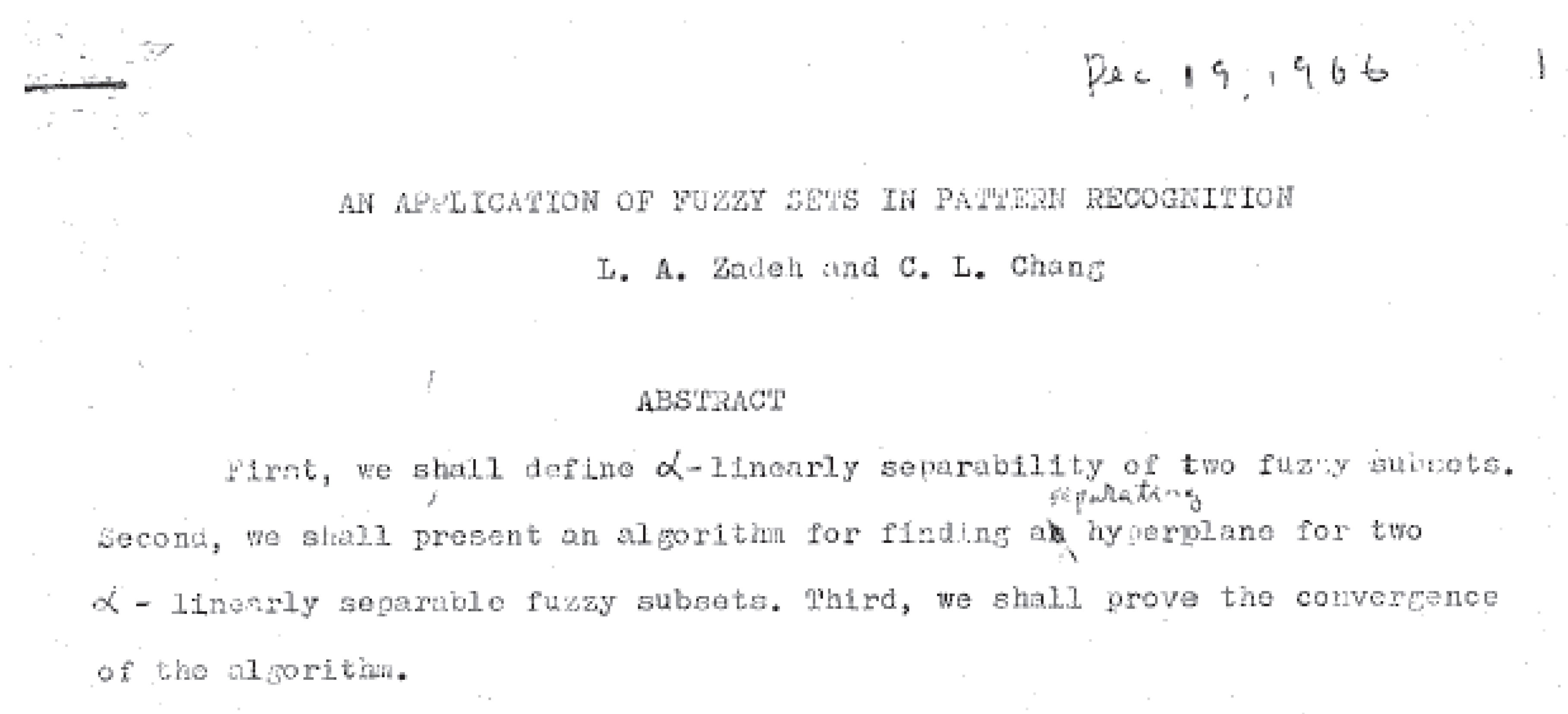
In 1962, the electrical engineer Chin-Liang Chang came from Taiwan to the US, and in 1964, to UC Berkeley to pursue his PhD under the supervision of Zadeh. In his thesis “Fuzzy Sets and Pattern Recognition” (See: http://www.eecs.berkeley.edu/Pubs/Dissertations/Faculty/zadeh.html), he extended the perception convergence theorem to fuzzy sets, he presented an algorithm for finding a separating hyperplane, and he proved its convergence in finite iterations under a certain condition. A manuscript by Zadeh and Chang entitled “An Application of Fuzzy Sets in Pattern Recognition” with a date of 19 December 1966 (see Figure 10) never appeared published in a journal, but it became part of Chang’s PhD thesis.
Rosenblatt heralded the perceptron as a universal machine in his publications, e.g., “For the first time, we have a machine which is capable of having original ideas. ... As a concept, it would seem that the perceptron has established, beyond doubt, the feasibility and principle of nonhuman systems which may embody human cognitive functions ... The future of information processing devices which operate on statistical, rather than logical, principles seems to be clearly indicated” [14]. “For the first time we have a machine which is capable of having original ideas”, he said in “The New Scientist”. “As an analogue of the biological brain the perceptron … seems to come closer to meeting the requirements of a functional explanation of the nervous system than any system previously proposed” [30] (p. 1392), he continued. To the New York Times, he said, “in principle it would be possible to build brains that could reproduce themselves on an assembly line and which would be conscious of their existence” [31] (p. 25).
The euphoria came to an abrupt halt in 1969, however, when Marvin Minsky and Seymour Papert completed their study of perceptron networks, and published their findings in a book [32]. The results of the mathematical analysis to which they had subjected Rosenblatt’s perceptron were devastating: “Artificial neuronal networks like those in Rosenblatt’s perceptron are not able to overcome many different problems! For example, it could not discern whether the pattern presented to it represented a single object or a number of intertwined but unrelated objects. The perceptron could not even determine whether the number of pattern components was odd or even. Yet this should have been a simple classification task that was known as a ‘parity problem’. What we showed came down to the fact that a Perceptron cannot put things together that are visually nonlocal”, Minsky said to Bernstein [33].
Specifically, in their analysis they argued, firstly, that the computation of the XOR had to be done with multiple layers of perceptrons, and, secondly, that the learning algorithm that Rosenblatt proposed did not work for multiple layers.
The so-called “XOR”, the either–or operator of propositional logic presents a special case of the parity problem that, thus, cannot be solved by Rosenblatt’s perceptron. Therefore, the logical calculus realized by this type of neuronal networks was incomplete.
The truth table (Table 1) of the logical functor, XOR, allocates the truth value “0” to the truth values of the two statements, x1 and x2, when their truth values agree, and the truth value “1” when they have different truth values.
x1 and x2 are components of a vector of the intermediate layer of a perceptron, so they can be interpreted, for example, as the coding of a perception by the retina layer. So, y = x1 XOR x2 is the truth value of the output neuron, which is calculated according to the truth table. The activity of x1 and x2 determines this value. It is a special case of the parity problem in this respect. For an even number, i.e., when both neurons are active or both are inactive, the output is 0, while for an odd number, where just one neuron is active, the value is 1.
To illustrate this, the four possible combinations of 0 and 1 are entered into a rectangular coordinate system of x1 and x2, and marked with the associated output values. In order to see that, in principle, a perceptron cannot learn to provide the output values demanded by XOR, the sum of the weighted input values is calculated by w1x1 + w2x2.
The activity of the output depends on whether this sum is larger or smaller than the threshold value, which results in the plane extending between x1 and x2 as follows:
Θ = w1x1 + w2x2, which results in: x2 = −w1 w2 x1 + Θ w2.
This is the equation of a straight line in which, on one side, the sum of the weighted input values is greater than the threshold value (w1x1 + w2x2 > Θ) and the neuron is, thus, active (fires); however, on the other side, the sum of the weighted input values is smaller than the threshold value (w1x1 + w2x2 < Θ), and the neuron is, thus, not active (does not fire).
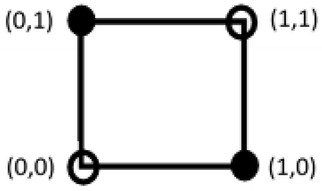
However, the attempt to find precisely those values for the weights, w1 and w2, where the associated line separates the odd number with (0, 1) and (1, 0) from the even number with (0, 0), and (1, 1) must fail (see Figure 10). The proof is very easy to demonstrate by considering all four cases:
- x1 = 0, x2 = 1: y should be 1 → w1 · 0 + w2 · 1 ≥ Θ → neuron is active!
- x1 = 1, x2 = 0: y should be 1 → w1 · 1 + w2 · 0 ≥ Θ → neuron is active!
- x1 = 0, x2 = 0: y should be 0 → w1 · 0 + w2 · 0 < Θ → neuron is inactive!
- x1 = 1, x2 = 1: y should be 0 → w1 · 1 + w2 · 1 < Θ → neuron is inactive!
Adding the first two equations results in w1 + w2 ≥ 2Θ.
From the last two equations comes Θ > w1 + w2 ≥ 2Θ, and so Θ > 2Θ.
This applies only where Θ < 0. This is a contradiction of w10 + w20 < Θ. Q.E.D.
The limits of the Rosenblatt perceptron were, thus, demonstrated, and they were very narrow, for it was not even able to classify linearly separable patterns. In their book, Minsky and Papert estimated that more than 100 groups of researchers were working on perceptron networks or similar systems all over the world at that time. In their paper “Adaptive Switching Circuits”, Bernard Widrow and Marcian Edward Hoff publicized the linear adaptive neuron model, ADALINE, an adaptive system that was quick and precise thanks to a more advanced learning process which today is known as the “Delta rule” [34]. In his 1958 paper “Die Lernmatrix”, German physicist, Karl Steinbuch, introduced a simple technical realization of associative memories, the predecessor of today’s neuronal associative memories [35]. In 1959, the paper “Pandemonium” by Oliver Selfridge was published in which dynamic, interactive mechanisms were described that used filtering operations to classify images by means of “significant criteria, e.g., four corners to identify a square”. He expected to develop a system that will also recognize “other kinds of features, such as curvature, juxtaposition of singular points, that is, their relative bearings and distances and so forth” [36] (p. 93), [37]. Already since 1955, Wilfred Kenelm Taylor in the Department of Anatomy of London’s University College aimed to construct neural analogs to study theories of learning [38].
However, the publication of Minsky and Papert’s book disrupted research in artificial neural networks for more than a decade. Because of their fundamental criticism, many of these projects were shelved or at least modified in the years leading up to 1970. In the 15 years that followed, almost no research grants were approved for projects in the area of artificial neuronal networks, especially not by the US Defense Department for DARPA (Defense Advanced Research Projects Agency. The pattern recognition and learning networks faltered on elementary questions of logic in which their competitor, the digital computer, proved itself immensely powerful.
7. Outlook
The disruption of artificial neural networks research later became known as the “AI winter”, but artificial neural networks were not killed by Minsky and Papert. In 1988, Seymour Papert did wonder whether this was actually their plan: “Did Minsky and I try to kill connectionism, and how do we feel about its resurrection? Something more complex than a plea is needed. Yes there was some hostility in the energy behind the research reported in Perceptrons, and there is some degree of annoyance at the way the new movement has developed; part of our drive came, as we quite plainly acknowledged in our book, from the fact that funding and research energy were being dissipated on what still appear to me (since the story of new, powerful network mechanisms is seriously exaggerated) to be misleading attempts to use connectionist methods in practical applications. But most of the motivation for Perceptrons came from more fundamental concerns many of which cut cleanly across the division between networkers and programmers” [39] (p. 346).
Independent of artificial neural networks, fuzzy pattern classification became popular in the 1960s. Looking to the emerging field of biomedical engineering, the Argentinian mathematician Enrique Ruspini, a graduate student at the University of Buenos Aires, came “across, however, early literature on numerical taxonomy (then focused on “Biological Systematics”, which was mainly concerned with classification of biological species), a field where its seminal paper by Sokal (Robert Reuven Sokal was an Austrian-American biostatistician and entomologist) and Sneath (Peter Henry Andrews Sneath was a British microbiologist. He began working on numerical methods for classifying bacteria in the late 1950s) had been published in 1963” [40,41]. In the interview, he continued, “It is interesting to note that the field was so young that, at the point, there were not even accepted translations to Spanish of words such as ‘pattern’ or ‘clustering’. After trying to understand and formulate the nature of the problem (I am a mathematician after all!), it was clear to me that the stated goal of clustering procedures (‘classify similar objects into the same class and different objects into different classes’) could not be attained within the framework of classical set theory. By sheer accident I walked one day into the small library of the Department of Mathematics at the School of Science. Perusing through the new-arrivals rack I found the 1965 issue of Information and Control with Lotfi Zadeh’s seminal paper [25]. It was clear to me and my colleagues that this was a much better framework to consider and rigorously pose fuzzy clustering problems. Drawing also from results in the field of operations research I was soon able to pose the clustering problem in terms of finding the optimal solution of a continuous variable system with well-defined performance criteria and constraints.” [17] (p. 2f)
In the quoted double-interview, Jim Bezdek also looked back: “So, when I got to Cornell in 1969, the same year that the Minsky and Papert book came out, he [Henry David Block] and others (including his best friend, Bernie Widrow, I might add), were in a funk about the apparent death of the ANNs (artificial neural networks). Dave wanted to continue in this field, but funding agencies were reluctant to forge ahead with NNs in the face of the damning damning indictment (which in hindsight was pretty ridiculous) by Minsky and Papert. About 1970, Richard Duda sent Dave a draft of his book with Peter Hart, the now and forever famous ‘Duda and Hart’ book on Pattern Classification and Scene Analysis, published in 1973 [42,43]. Duda asked Dave to review it. Dave threw it in Joe Dunn’s inbox, and from there it made its way to mine. So I read it—cover to cover—trying to find corrections, etc. whilst simultaneously learning the material, and that’s how I entered the field of pattern recognition”. Bezdek included his best Dave Block story: “In maybe 1971, Dave and I went over to the Cornell Neurobiology Lab in Triphammer Woods, where we met a young enterprising neuroscientist named Howard Moraff, who later moved to the NSF, where he is (I think still today). Howard was hooking up various people to EEG sensor nodes on their scalps—16 sites at that time—and trying to see if there was any information to be gleaned from the signals. We spent the day watching him, talking to him, etc. Dave was non-committal to Howard about the promise of this enterprise, but as we left the building, Dave turned to me and said ‘Maybe there is some information in the signals Jim, but we are about 50 years too early’”. Then, he commented this: “I have told this story many times since then (43 years ago now), and I always end it by saying this: ‘And if Dave could see the signals today, given our current technology, what do you think he would say now? He would say «Jim, we are about 50 years too soon»’. So, the bottom line for me in 1971 was: don’t do NNS, but clustering and classifier design with OTHER paradigms is ok. As it turned out, however, I was out of the frying pan of NNs, and into the fire of Fuzzy Sets, which was in effect a (very) rapid descent into the Maelstrom of probabilistic discontent” [17] (p. 5f). (NFS: National science Foundation, EEG: Electroencephalography)
Since 1981, the psychologists, James L. McClelland and David E. Rumelhart, applied artificial neural networks to explain cognitive phenomena (spoken and visual word recognition). In 1986, this research group published the two volumes of the book “Parallel Distributed Processing: Explorations in the Microstructure of Cognition” [44]. Already in 1982, John J. Hopfield, a biologist and Professor of Physics at Princeton, CalTech, published the paper “Neural networks and physical systems with emergent collective computational abilities” [45] on his invention of an associative neural network (now more commonly known as the “Hopfield Network”), i.e., feedback networks that have only one layer that is both input, as well as output layer, and each of the binary McCulloch–Pitts neurons is linked with every other, except itself. McClelland’s research group could show that perceptrons with more than one layer can realize the logical calculus; multilayer perceptrons were the beginning of the new direction in AI: parallel distributed processing.
In the mid-1980s, traditional AI explored their limitations, and with “more powerful hardware” (e.g., parallel architectures) and “new advances made in neural modelling learning methods” (e.g., feedforward neural networks with more than one layer, i.e., multilayer perceptrons), artificial neural modeling has awakened new interest in the fields of science, industry, and governments. In Japan, this resulted in the Sixth Generation Computing Project that started in 1986 [46], in Europe the following year, the interdisciplinary project “Basic Research in Adaptive Intelligence and Neurocomputing” (BRAIN) of the European Economic Community [47], and in the US, the DARPA Neural Network Study (1987–1988) [48].
Today, among other algorithms, e.g., decision trees and random forests, artificial neural networks are enormously successful in data mining, machine learning, and knowledge discovery in databases.
Funding
This research received no external funding.
Acknowledgments
I would like to thank James C. Bezdek, Enrique H. Ruspini, and Chin-Liang Chang for giving interviews in the year 2014 and helpful discussions. I am very thankful to Lotfi A. Zadeh, who sadly passed away in September 2017, for many interviews and discussions in almost 20 years of historical research work. He has encouraged and supported me with constant interest and assistance, and he gave me the opportunity to collect a “digital fuzzy archive” with historical sources.
Conflicts of Interest
The authors declare no conflict of interest.
References
- Rosen, C.A. Pattern Classification by Adaptive Machines. Science 1967, 156, 38–44. [Google Scholar] [CrossRef] [PubMed]
- Bellman, R.E.; Kalaba, R.; Zadeh, L.A. Abstraction and Pattern Classification. Memorandum RM-4307-PR; The RAND Corporation: Santa Monica, CA, USA, 1964. [Google Scholar]
- Bellman, R.E.; Kalaba, R.; Zadeh, L.A. Abstraction and Pattern Classification. J. Math. Anal. Appl. 1966, 13, 1–7. [Google Scholar] [CrossRef]
- Minsky, M.L. Steps toward Artificial Intelligence. Proc. IRE 1960, 49, 8–30. [Google Scholar] [CrossRef]
- Zadeh, L.A. From Circuit Theory to System Theory. Proc. IRE 1962, 50, 856–865. [Google Scholar] [CrossRef]
- Eidelheit, M. Zur Theorie der konvexen Mengen in linearen normierten Räumen. Studia Mathematica 1936, 6, 104–111. [Google Scholar] [CrossRef]
- Zadeh, L.A. On the Identification Problem. IRE Trans. Circuit Theory 1956, 3, 277–281. [Google Scholar] [CrossRef]
- Zadeh, L.A. What is optimal? IRE Trans. Inf. Theory 1958, 1. [Google Scholar]
- Zadeh, L.A. Optimality and Non-Scalar-Valued Performance Criteria. IEEE Trans. Autom. Control 1963, 8, 59–60. [Google Scholar] [CrossRef]
- McCulloch, W.S.; Pitts, W. A logical calculus of the ideas immanent in nervous activity. Bull. Math. Biophys. 1943, 5, 115–133. [Google Scholar] [CrossRef]
- Hebb, D.O. The Organization of Behavior: A Neuropsychological Theory; Wiley and Sons: New York, NY, USA, 1949. [Google Scholar]
- Hayek, F.A. The Sensory Order: An Inquiry into the Foundations of Theoretical Psychology; University of Chicago Press: Chicago, IL, USA, 1952. [Google Scholar]
- Rosenblatt, F. The Perceptron. A Theory of Statistical Separability in Cognitive Systems, (Project PARA); Report No. VG-1196-G-1; Cornell Aeronautical Laboratory: New York, NY, USA, 1958. [Google Scholar]
- Rosenblatt, F. The Perceptron. A Probabilistic Model for Information Storage and Organization in the Brain. Psychol. Rev. 1958, 65, 386–408. [Google Scholar] [CrossRef] [PubMed]
- Rosenblatt, F. A Probabilistic Model for Visual Perception. Acta Psychol. 1959, 15, 296–297. [Google Scholar] [CrossRef]
- Rosenblatt, F. The Design of an Intelligent Automaton. Res. Trends 1958, VI, 1–7. [Google Scholar]
- Seising, R. On the History of Fuzzy Clustering: An Interview with Jim Bezdek and Enrique Ruspini. IEEE Syst. Man Cybern. Mag. 2015, 1, 20–48. [Google Scholar] [CrossRef]
- Block, H.D. The Perceptron: A Model for Brain Functioning I. Rev. Mod. Phys. 1962, 34, 123–135. [Google Scholar] [CrossRef]
- Novikoff, A. On Convergence Proofs for Perceptions. In Proceedings of the Symposium on Mathematical Theory of Automata; Polytechnic Institute of Brooklyn: Brooklyn, NY, USA, 1962; Volume XII, pp. 615–622. [Google Scholar]
- Aizerman, M.A.; Braverman, E.M.; Rozonoer, L.I. Theoretical Foundations of the Potential Function Method in Pattern Recognition Learning. Autom. Remote Control 1964, 25, 821–837. [Google Scholar]
- Aizerman, M.A.; Braverman, E.M.; Rozonoer, L.I. The Method of Potential Function for the Problem of Restoring the Characteristic of a Function Converter from Randomly Observed Points. Autom. Remote Control 1964, 25, 1546–1556. [Google Scholar]
- Aizerman, M.A.; Braverman, E.M.; Rozonoer, L.I. The Probability Problem of Pattern Recognition Learning and the Method of Potential Functions. Autom. Remote Control 1964, 25, 1175–1190. [Google Scholar]
- Rosen, J.B. Pattern Separation by Convex Programming; Technical Report No. 30; Applied Mathematics and Statistics Laboratories, Stanford University: Stanford, CA, USA, 1963. [Google Scholar]
- Rosen, J.B. Pattern Separation by Convex Programming. J. Math. Anal. Appl. 1965, 10, 123–134. [Google Scholar] [CrossRef]
- Zadeh, L.A. Fuzzy Sets. Inf. Control 1965, 8, 338–353. [Google Scholar] [CrossRef]
- Zadeh, L.A. Fuzzy Sets and Systems. In System Theory; Microwave Research Institute Symposia Series XV; Fox, J., Ed.; Polytechnic Press: Brooklyn, NY, USA, 1965; pp. 29–37. [Google Scholar]
- Zadeh, L.A. Shadows of Fuzzy Sets. Problemy peredachi informatsii. In Akadamija Nauk SSSR Moskva; Problems of Information Transmission: A Publication of the Academy of Sciences of the USSR; The Faraday Press: New York, NY, USA, 1966; Volume 2. [Google Scholar]
- Zadeh, L.A. Shadows of Fuzzy Sets. In Notes of System Theory; Report No. 65-14; Electronic Research Laboratory, University of California Berkeley: Berkeley, CA, USA, 1965; Volume VII, pp. 165–170. [Google Scholar]
- Zadeh, L.A. Fuzzy Sets; ERL Report No. 64-44; University of California at Berkeley: Berkeley, CA, USA, 1964. [Google Scholar]
- Rival. The New Yorker. 6 December 1958, p. 44. Available online: https://www.newyorker.com/magazine/1958/12/06/rival-2 (accessed on 21 June 2018).
- New Navy Device learns by doing. Psychologist Shows Embryo of Computer Designed to Read and Crow Wise. New York Times, 7 July 1958; 25.
- Minsky, M.L.; Papert, S. Perceptrons; MIT Press: Cambridge, MA, USA, 1969. [Google Scholar]
- Bernstein, J.; Profiles, A.I. Marvin Minsky. The New Yorker, 14 December 1981; 50–126. [Google Scholar]
- Widrow, B.; Hoff, M.E. Adaptive Switching Circu its, IRE Wescon Convention Record. New York IRE 1960, 4, 96–104. [Google Scholar]
- Steinbuch, K. Die Lernmatrix, Kybernetik; Springer: Berlin, Germany, 1961; Volume 1. [Google Scholar]
- Selfridge, O.G. Pattern Recognition and Modern Computers. In Proceedings of the AFIPS ‘55 Western Joint Computer Conference, Los Angeles, CA, USA, 1–3 March 1955; ACM: New York, NY, USA, 1955; pp. 91–93. [Google Scholar]
- Selfridge, O.G. Pandemonium: A Paradigm for Learning. In Mechanisation of Thought Processes: Proceedings of a Symposium Held at the National Physical Laboratory on 24th, 25th and 27th November 1958; National Physical Laboratory, Ed.; Her Majesty’s Stationery Office: London, UK, 1959; Volume I, pp. 511–526. [Google Scholar]
- Taylor, W.K. Electrical Simulation of Some Nervous System Functional Activities. Inf. Theory 1956, 3, 314–328. [Google Scholar]
- Papert, S.A. One AI or many? In The Philosophy of Mind; Beakley, B., Ludlow, P., Eds.; MIT Press: Cambridge, MA, USA, 1992. [Google Scholar]
- Sokal, R.R.; Sneath, P.H.A. Principles of numerical Taxonomy; Freeman: San Francisco, NC, USA, 1963. [Google Scholar]
- Sokal, R.R. Numerical Taxonomy the Principles and Practice of Numerical Classification; Freeman: San Francisco, CA, USA, 1973. [Google Scholar]
- Duda, R.O.; Hart, P.E. Pattern Classification and Scene Analysis, 2nd ed.; Wiley: Hoboken, NJ, USA, 1973. [Google Scholar]
- Duda, R.O.; Hart, P.E.; Stork, D.G. Pattern Classification; Wiley: Hoboken, NJ, USA, 2000. [Google Scholar]
- Rumelhart, D.E.; McClelland, J.L.; The PDP Research Group. Parallel Distributed Processing. Explorations in the Microstructure of Cognition; MIT Press: Cambridge, MA, USA, 1986. [Google Scholar]
- Hopfield, J.J. Neural networks and physical systems with emergent collective computational abilities. Proc. Natl. Acad. Sci. USA 1982, 79, 2554–2558. [Google Scholar] [CrossRef] [PubMed]
- Gaines, B. Sixth generation computing. A conspectus of the Japanese proposals. Newsletter 1986, 95, 39–44. [Google Scholar]
- Roman, P. The launching of BRAIN in Europe. In Europea Science Notes; US Office of Naval Research: London, UK, 1987; Volume 41. [Google Scholar]
- DARPA. Neural Network Study; AFCEA International Press: Washington, DC, USA, 1988. [Google Scholar]
Figure 1.
The points (0,1) and (1,0) are not linearly separable.

Figure 2.
Lotfi A. Zadeh, undated photo, approximately 1950s, photo credit: Fuzzy archive Rudolf Seising.
Figure 2.
Lotfi A. Zadeh, undated photo, approximately 1950s, photo credit: Fuzzy archive Rudolf Seising.


Figure 4.
The set of noninferior points on the boundary of C [9].
Figure 4.
The set of noninferior points on the boundary of C [9].

Figure 5.
Organization of a biological brain and a perceptron [16] (p. 2), the picture was modified for better readability).
Figure 5.
Organization of a biological brain and a perceptron [16] (p. 2), the picture was modified for better readability).

Figure 6.
Detailed organization of a single perceptron [16] (p. 3).
Figure 6.
Detailed organization of a single perceptron [16] (p. 3).

Figure 7.
Learning curves for three typical perceptrons [16] (p. 6).
Figure 7.
Learning curves for three typical perceptrons [16] (p. 6).

Figure 8.
Illustration to Zadeh’s view on pattern classification: the sign □ (or x, as Zadeh wrote) belongs with membership value, μO(O), to the “class” of Os and with membership value, μD(D), to the “class” of Ds.
Figure 8.
Illustration to Zadeh’s view on pattern classification: the sign □ (or x, as Zadeh wrote) belongs with membership value, μO(O), to the “class” of Os and with membership value, μD(D), to the “class” of Ds.

Figure 9.
Illustration of the separation theorem for fuzzy sets in E1 [25].
Figure 9.
Illustration of the separation theorem for fuzzy sets in E1 [25].

Figure 10.
Unpublished manuscript (excerpt) of Zadeh and Chang, 1966. (Fuzzy Archive, Rudolf Seising).
Figure 10.
Unpublished manuscript (excerpt) of Zadeh and Chang, 1966. (Fuzzy Archive, Rudolf Seising).


Table 1.
Truth table of the logical operator XOR.
| x1 | x2 | x1 XOR x2 |
|---|---|---|
| 0 | 0 | 0 |
| 0 | 1 | 1 |
| 1 | 0 | 1 |
| 1 | 1 | 0 |
© 2018 by the author. Licensee MDPI, Basel, Switzerland. This article is an open access article distributed under the terms and conditions of the Creative Commons Attribution (CC BY) license (http://creativecommons.org/licenses/by/4.0/).
Share and Cite
MDPI and ACS Style
Seising, R. The Emergence of Fuzzy Sets in the Decade of the Perceptron—Lotfi A. Zadeh’s and Frank Rosenblatt’s Research Work on Pattern Classification. Mathematics 2018, 6, 110. https://doi.org/10.3390/math6070110
AMA Style
Seising R. The Emergence of Fuzzy Sets in the Decade of the Perceptron—Lotfi A. Zadeh’s and Frank Rosenblatt’s Research Work on Pattern Classification. Mathematics. 2018; 6(7):110. https://doi.org/10.3390/math6070110
Chicago/Turabian StyleSeising, Rudolf. 2018. "The Emergence of Fuzzy Sets in the Decade of the Perceptron—Lotfi A. Zadeh’s and Frank Rosenblatt’s Research Work on Pattern Classification" Mathematics 6, no. 7: 110. https://doi.org/10.3390/math6070110
Note that from the first issue of 2016, this journal uses article numbers instead of page numbers. See further details here.