Accelerated Degradation Model of Nonlinear Wiener Process Based on Fixed Time Index

Abstract

In the process of extrapolating a lifetime distribution function under normal storage conditions through nonlinear accelerated degradation data, time indexes under the normal storage conditions are usually set to the mean value of time indexes under various accelerated stresses. However, minor differences in time indexes may lead to great changes in the assessment results. For such a problem, an accelerated degradation model of a nonlinear Wiener process based on a fixed time index is established first and meanwhile, the impact of the measurement error is considered. Then, the probability density function is normalized, and multiple unknown parameters are estimated by using fminsearch function in MATLAB and multiple iterations. Finally, the model is validated by accelerated degradation test data of accelerometers and the O-type rubber sealing rings. The results show that there is a difference of 30,710 h for accelerometers between the mean time to failure under normal storage conditions obtained by the proposed method and the mean time to failure when the time indexes are the mean value of those under various accelerated stresses, and the main cause of the difference is compared and analyzed. A similar phenomenon is observed in the case study of O-type rubber sealing rings.

1. Introduction

For most products, product performance will degrade constantly, as the service time increases during actual use. Parameters that can represent performance information of a product are referred to as degradation values, and the product will be failed when the performance degradation values reach a certain extent. The lifetime information and the reliability function of the product can be obtained through statistics, analysis and calculation on a degradation path of the product. However, some products are characterized in long life, high reliability, long test period, and high test cost, thus being difficult to meet the requirement of rapidity. Therefore, an accelerated test method is required to test samples with the unchanged failure mechanism under environmental conditions or working stresses more severe than use conditions, thus accelerating the degradation of products. Finally, the lifetime information of the products under the design or use conditions is obtained by extrapolation [1,2].

Degradation paths of products are classified into linear degradation paths and nonlinear degradation paths. The nonlinear degradation paths are more universal than the linear degradation paths [3]. Moreover, the linear degradation paths can also be considered as special forms of nonlinear degradation paths. Therefore, models based on nonlinear degradation paths have been widely applied. The Wiener process is a random process, and the degradation process of the product is described using the drift Wiener process that can not only represent the influence of stress on the product, but also describe the uncertainty of the degradation process. At present, there are 4 types of common nonlinear Wiener processes [4]. The first type is a logarithmic transformation model of degradation value, which is mainly applicable to take a logarithm of the degradation value so that the degradation path is linear [5]. The second type is a time scale transformation model, with which the degeneration time scale is transformed first, and then modeling is carried out using a linear Wiener process model in the transformed time scale [6]. The third type is a generalized Wiener model, with which solutions of unknown parameters of accelerated degradation data under multiple stresses will be especially more complicated due to a large number of parameters [7,8]. The fourth type is a nonlinear Wiener degradation model proposed in reference [9], in which a drift value is a nonlinear function of time. The first type and the second type have certain limitations for general nonlinear degradation data, while the third type has too many unknown parameters in the case of accelerated degradation; therefore, this paper mainly adopts the nonlinear Wiener process model proposed in reference [9].

On the basis of the nonlinear Wiener process proposed in reference [9], an accelerated degradation model based on the nonlinear Wiener process is established in reference [10], in which the Arrhenius equation is used to extrapolate the mean value and variance of the drift parameter, as well as the diffusion parameter. Thus, the drift parameter and the diffusion parameter under normal stress condition are obtained by Arrhenius equation, and the time index under normal stress condition is set to the mean value of time indexes under three accelerated stresses. However, the nonlinear Wiener process is very sensitive to the time index, and a small change in the time index can cause dramatic changes in other parameters, especially for the degradation parameters under the constant stress after extrapolation. In this paper, the time index of the nonlinear Wiener process is determined as a fixed value, an accelerated degradation model based on the completely accelerated degradation data is established, and the probability density function (PDF) of the first-passage time is normalized using the normalization method.

Meanwhile, there are measurement errors in the process of collecting the degradation data. Whitmore [11] proposed a degradation model based on time scale transformed nonlinear Wiener process with measurement errors which are assumed to follow normal distribution and are independent of the degradation process. However, the work does not make full use of the degradation data so that a new degradation model including measurement errors was driven [12]. Other degradation model based on Wiener process incorporating measurement errors can refer to reference [13,14,15,16]. Therefore, the impacts of measurement errors on the proposed model are taken into account. Finally, the results obtained by this model are compared with those obtained by the model in reference [10].

2. Accelerated Degradation Model Based on Nonlinear Wiener Process

2.1. Nonlinear Wiener Process

As can be seen from the reference [9], the degradation value of the product at the moment t is X(t), as expressed by the following expression

$$X\left(t\right)=X\left(0\right)+a{\displaystyle {\int }_0^t\mu \left(u;\mathit{\vartheta }\right)du}+{\sigma }_{B}B\left(t\right)$$

(1)

where, X(0) denotes the initial degradation value, which is generally 0, and can be converted using X(t) − X(0) (in an ascending case) or X(0) − X(t) (in a descending case) if it is not 0, a is a random parameter unrelated to the degradation time and denotes the difference between samples, that is, different individuals have different a; $\mu \left(t;\mathit{\vartheta }\right)$ denotes a function of the time t, and this model is a general Wiener model when $\mu \left(u;\mathit{\vartheta }\right)$ = 1; $\mathit{\vartheta }$ denotes the vector of unknown parameters; σ_B denotes the diffusion parameter; and B(t) denotes the standard Brownian motion.

When the degradation value of the product exceeds a failure threshold w, the product cannot meet usage requirements and is thus failed. As for the first-passage time, the time at which the degradation value reaches the failure threshold w for the first time is generally defined as the lifetime of the product, and when the parameter a is given, the lifetime T of the product can be expressed as:

$$T=\inf \left\{t:X\left(t|a\right)\ge w|X\left(0\right)<w\right\}$$

The probability density function of the lifetime T is

$$g_{T|a}\left(t|a\right)\cong \frac{1}{\sqrt{2\pi t}}\left(\frac{S\left(t\right)}{t}+\frac{a}{{\sigma }_B}\mu \left(u;\vartheta \right)\right)\exp \left[-\frac{S^2\left(t\right)}{2t}\right]$$

where

$$S\left(t\right)=\left(w-a{\displaystyle {\int }_0^t\mu \left(u;\mathit{\vartheta }\right)du}\right)/{\sigma }_B$$

By taking the impact of the random parameter a into consideration, the probability density function of the lifetime T can be obtained through a total probability formula

$$g_T\left(t\right)={\displaystyle {\int }_a{g}_{T|a}\left(t|a\right)p\left(a\right)da}=E_a\left[g_{T|a}\left(t|a\right)\right]$$

where p(a) is the probability density function of the random variable a.

It is assumed that the random variable a follows a normal distribution, $a~N\left({\mu }_a,{\sigma }_a^2\right)$; $\mu \left(u;\mathit{\vartheta }\right)=b{t}^{b-1}$ is a common form, where b is the parameter in time scale function, and when it is substituted into the foregoing formula, the probability density function of the lifetime T can be obtained as

$$g_T\left(t\right)\cong \frac{1}{\sqrt{2\pi t^3\left({\sigma }_a^2{t}^{2b-1}+{\sigma }_B^2\right)}}\times \left(w-\left(t^b-b{t}^b\right)\frac{w{\sigma }_a^2{t}^{b-1}+{\mu }_a{\sigma }_B^2}{{\sigma }_a^2{t}^{2b-1}+{\sigma }_B^2}\right)\times \exp \left[-\frac{{\left(w-{\mu }_a{t}^b\right)}^2}{2t\left({\sigma }_a^2{t}^{2b-1}+{\sigma }_B^2\right)}\right]$$

(2)

The probability density function $g_T\left(t\right)$ needs to meet ${\displaystyle {\int }_{\mathsf{\Omega }}{g}_T\left(t\right)}=1$ [8], and therefore, the probability density function can be normalized to obtain

$$f_T\left(t\right)\cong \frac{1}{A_T}{g}_T\left(t\right)$$

(3)

where $A_T={\displaystyle {\int }_0^{\infty }{g}_T\left(t\right)dt}$. The expression of $g_T\left(t\right)$ is complicated, and thus it is difficult to obtain the analytic expression of A_T.

2.2. Accelerated Degradation Model

The mean value and variance of the random variable a, as well as the diffusion parameter σ_B under different accelerated stresses are all related to the accelerated stresses. Their correlational relationships are expressed as follows:

$${\mu }_a={\alpha }_1\varsigma \left(S;{\beta }_1\right)$$

(4)

$${\sigma }_a^2={\alpha }_2\varsigma \left(S;{\beta }_2\right)$$

(5)

$${\sigma }_B^2={\alpha }_3\varsigma \left(S;{\beta }_3\right)$$

(6)

where, $\varsigma \left(S;\beta \right)=\exp \left(\beta /S\right)$ [17] when the accelerated stresses are temperature stresses, and $\varsigma \left(S;\beta \right)=S^{\beta }$ [18] when the accelerated stresses are electrical stresses.

It is assumed that there are K accelerated stresses in total in the accelerated degradation test, the number of samples under the kth stress is N_k(k = 1, 2, …, K), and the number of detections of the ith sample under the kth stress is M_ki. Therefore, the degradation value of the product at a measurement time point t_kij is X_kij

$$X_{kij}\left(t_{kij}\right)=a_{ki}\left(S_k\right){\displaystyle {\int }_0^{t_{kij}}\mu \left(u;\mathit{\vartheta }\right)du}+{\sigma }_B\left(S_k\right)B\left(t_{kij}\right)$$

where i = 1, 2, …, N_k; and j = 1, 2, …, M_ki.

3. Estimation of Unknown Parameters

3.1. Method for Estimating Total Unknown Parameters

In the process of detecting the degradation value, measurement errors are inevitably introduced in a measurement value [19] of the degradation value due to the inherent errors of measurement instrument, operation errors of measurement personnel, and other random factors. Therefore, the degradation value obtained by the test is not the real degradation value of the product. Impacts of the measurement errors need to be taken into consideration in the process of estimating the unknown parameters; therefore, the measured degradation value and the real degradation value have the following relationship:

$$Y\left(t\right)=X\left(t\right)+\epsilon$$

(7)

where ε denotes the measurement error and is generally assumed as the random variable $\epsilon ~N\left(0,{\sigma }_{\epsilon }^2\right)$ following the normal distribution, and the same assumption can be seen in the references [12,17]. At the same time, the measurement error is independent of the real degradation value. An observed value of the degradation value of the ith sample under the kth stress at the jth detection time point is marked as y_kij.

As can be seen from the above analysis that unknown parameters $\mathbf{\Theta }=\left\{{\alpha }_1,{\alpha }_2,{\alpha }_3,{\beta }_1,{\beta }_2,{\beta }_2,b,{\sigma }_{\epsilon }^2\right\}$ need to be solved in the model, and the unknown parameters are estimated using the independence feature of the degradation increment in the Wiener process. The degradation increment of the ith sample under the kth stress can be expressed as $\mathsf{\Delta }{\mathit{y}}_{ki}={\left\{\mathsf{\Delta }{y}_{ki1},\cdots ,\mathsf{\Delta }{y}_{kij},\cdots ,\mathsf{\Delta }{y}_{ki{M}_{ki}}\right\}}^{\mathrm{T}}$, $\mathsf{\Delta }{y}_{ki1}=y_{ki1}$, $\mathsf{\Delta }{y}_{kij}=y_{kij}-y_{ki\left(j-1\right)}$, the corresponding time increment matrix can be expressed as ${\mathit{T}}_{ki}={\left\{\mathsf{\Delta }{\tau }_{ki1},\cdots ,\mathsf{\Delta }{\tau }_{kij},\cdots ,\mathsf{\Delta }{\tau }_{ki{M}_{ki}}\right\}}^{\mathrm{T}}$, $\mathsf{\Delta }{\tau }_{ki1}=t_{ki1}^b$, $\mathsf{\Delta }{\tau }_{kij}=t_{kij}^b-t_{ki\left(j-1\right)}^b$, and it can be obtained according to the independence assumption that the degradation increment matrix $\mathsf{\Delta }{\mathit{y}}_{ki}$ follows a multivariate normal distribution with mean value and covariance

$${\mathit{\mu }}_{ki}={\alpha }_1\varsigma \left(S_k;{\beta }_1\right){\mathit{T}}_{ki}$$

$${\mathbf{\Sigma }}_{ki}={\alpha }_2\varsigma \left(S_k;{\beta }_2\right){\mathit{T}}_{ki}{{\mathit{T}}_{ki}}^{\prime }+{\mathbf{\Omega }}_{ki}$$

where

$${\mathbf{\Omega }}_{ki}=\left[\begin{array}{ccccc}{\omega }_{11}& \cdots & {\omega }_{1q}& \cdots & {\omega }_{1M_{ki}}\\ ⋮& ⋮& ⋮& ⋮& ⋮\\ {\omega }_{p1}& \cdots & {\omega }_{pq}& \cdots & {\omega }_{p{M}_{ki}}\\ ⋮& ⋮& ⋮& ⋮& ⋮\\ {\omega }_{M_{ki}1}& \cdots & {\omega }_{M_{ki}q}& \cdots & {\omega }_{M_{ki}{M}_{ki}}\end{array}\right]$$

$${\omega }_{pq}=\{\begin{array}{ll}{\alpha }_3\varsigma \left(S_k;{\beta }_3\right)\mathsf{\Delta }{t}_{kip}+{\sigma }_{\epsilon }^2,& p=q=1;\\ {\alpha }_3\varsigma \left(S_k;{\beta }_3\right)\mathsf{\Delta }{t}_{kip}+2{\sigma }_{\epsilon }^2,& p=q>1;\\ -{\sigma }_{\epsilon }^2,& p=q+1 or p=q-1;\\ 0,& otherwise;\end{array}$$

where, $\mathsf{\Delta }{t}_{ki1}=t_{ki1}$, $\mathsf{\Delta }{t}_{kip}=t_{kip}-t_{ki\left(p-1\right)}$.

To simplify the calculation, let ${\tilde{\alpha }}_2={\alpha }_2/{\alpha }_3$, ${\tilde{\sigma }}_{\epsilon }^2={\sigma }_{\epsilon }^2/{\alpha }_3$, and therefore, ${\mathbf{\Sigma }}_{ki}={\alpha }_3{\tilde{\mathbf{\Sigma }}}_{ki};{\tilde{\mathbf{\Sigma }}}_{ki}={\tilde{\alpha }}_2\varsigma \left(S_k;{\beta }_2\right){\mathit{T}}_{ki}{{\mathit{T}}_{ki}}^{\prime }+{\tilde{\mathbf{\Omega }}}_{ki}$, correspondingly

$${\tilde{\mathbf{\Omega }}}_{ki}=\left[\begin{array}{ccccc}{\tilde{\omega }}_{11}& \cdots & {\tilde{\omega }}_{1q}& \cdots & {\tilde{\omega }}_{1M_{ki}}\\ ⋮& ⋮& ⋮& ⋮& ⋮\\ {\tilde{\omega }}_{p1}& \cdots & {\tilde{\omega }}_{pq}& \cdots & {\tilde{\omega }}_{p{M}_{ki}}\\ ⋮& ⋮& ⋮& ⋮& ⋮\\ {\tilde{\omega }}_{M_{ki}1}& \cdots & {\tilde{\omega }}_{M_{ki}q}& \cdots & {\tilde{\omega }}_{M_{ki}{M}_{ki}}\end{array}\right]$$

$${\tilde{\omega }}_{pq}=\{\begin{array}{ll}\varsigma \left(S_k;{\beta }_3\right)\mathsf{\Delta }{t}_{kip}+{\tilde{\sigma }}_{\epsilon }^2,& p=q=1;\\ \varsigma \left(S_k;{\beta }_3\right)\mathsf{\Delta }{t}_{kip}+2{\tilde{\sigma }}_{\epsilon }^2,& p=q>1;\\ -{\tilde{\sigma }}_{\epsilon }^2,& p=q+1 or p=q-1;\\ 0,& otherwise.\end{array}$$

Measurement values of degradation values of different samples are independent of one another, and the log-likelihood function for unknown parameters $\mathbf{\Theta }={\left\{{\alpha }_1,{\alpha }_2,{\alpha }_3,{\beta }_1,{\beta }_2,{\beta }_3,b,{\sigma }_{\epsilon }^2\right\}}^{\mathrm{T}}$ can be obtained

$$\begin{array}{ll}\ln L\left(\mathbf{\Theta }\right)=& -\frac{1}{2}\ln \left(2\pi \right){\displaystyle \sum _{k=1}^K{\displaystyle \sum _{i=1}^{N_k}{M}_{ki}}}-\frac{1}{2}{\displaystyle \sum _{k=1}^K{\displaystyle \sum _{i=1}^{N_k}\ln \left(\left|{\tilde{\mathbf{\Sigma }}}_{ki}\right|\right)}}-\frac{1}{2}{\displaystyle \sum _{k=1}^K{\displaystyle \sum _{i=1}^{N_k}{M}_{ki}\ln \left({\alpha }_3\right)}}\\ & -\frac{1}{2{\alpha }_3}{\displaystyle \sum _{k=1}^K{\displaystyle \sum _{i=1}^{N_k}{\left(\mathsf{\Delta }{\mathit{y}}_{ki}-{\alpha }_1\varsigma \left(S_k;{\beta }_1\right){\mathit{T}}_{ki}\right)}^{\prime }{\tilde{\mathbf{\Sigma }}}_{ki}^{-1}\left(\mathsf{\Delta }{\mathit{y}}_{ki}-{\alpha }_1\varsigma \left(S_k;{\beta }_1\right){\mathit{T}}_{ki}\right)}}\end{array}$$

Then, first-order derivatives are taken for the log-likelihood function $\ln L\left(\mathbf{\Theta }\right)$ with respect to α₁, α₃, thus obtaining

$$\frac{\partial \ln L\left(\mathbf{\Theta }\right)}{\partial {\alpha }_1}=\frac{1}{2{\alpha }_3}{\displaystyle \sum _{k=1}^K{\displaystyle \sum _{i=1}^{N_k}{\alpha }_1\varsigma \left(S_k;{\beta }_1\right){{\mathit{T}}_{ki}}^{\prime }{\tilde{\mathbf{\Sigma }}}_{ki}^{-1}{\mathit{y}}_{ki}}}-\frac{1}{2{\alpha }_3}{\displaystyle \sum _{k=1}^K{\displaystyle \sum _{i=1}^{N_k}{\left(\varsigma \left(S_k;{\beta }_1\right)\right)}^2{{\mathit{T}}_{ki}}^{\prime }{\tilde{\mathbf{\Sigma }}}_{ki}^{-1}{\mathit{T}}_{ki}}}$$

$$\frac{\partial \ln L\left(\mathbf{\Theta }\right)}{\partial {\alpha }_3}=-\frac{1}{2{\alpha }_3}{\displaystyle \sum _{k=1}^K{\displaystyle \sum _{i=1}^{N_k}{M}_{ki}}}+\frac{1}{2{\left({\alpha }_3\right)}^2}{\displaystyle \sum _{k=1}^K{\displaystyle \sum _{i=1}^{N_k}{\left(\mathsf{\Delta }{\mathit{y}}_{ki}-{\alpha }_1\varsigma \left(S_k;{\beta }_1\right){\mathit{T}}_{ki}\right)}^{\prime }{\tilde{\mathbf{\Sigma }}}_{ki}^{-1}\left(\mathsf{\Delta }{\mathit{y}}_{ki}-{\alpha }_1\varsigma \left(S_k;{\beta }_1\right){\mathit{T}}_{ki}\right)}}$$

Let $\partial \ln L\left(\mathbf{\Theta }\right)/\partial {\alpha }_1=0$, and the analytic expression of α₁ can be obtained as follows:

$${\widehat{\alpha }}_1=\frac{{\displaystyle \sum _{k=1}^K{\displaystyle \sum _{i=1}^{N_k}\varsigma \left(S_k;{\beta }_1\right){{\mathit{T}}_{ki}}^{\prime }{\tilde{\mathbf{\Sigma }}}_{ki}^{-1}{\mathit{y}}_{ki}}}}{{\displaystyle \sum _{k=1}^K{\displaystyle \sum _{i=1}^{N_k}{\left(\varsigma \left(S_k;{\beta }_1\right)\right)}^2{{\mathit{T}}_{ki}}^{\prime }{\tilde{\mathbf{\Sigma }}}_{ki}^{-1}{\mathit{T}}_{ki}}}}$$

(8)

Substitute ${\widehat{\alpha }}_1$ into the first-order derivative of log-likelihood function $\ln L\left(\mathbf{\Theta }\right)$ with respect to α₃ and let it be equal to 0, thus obtaining the analytic expression of α₃

$${\widehat{\alpha }}_3=\frac{1}{{\displaystyle \sum _{k=1}^K{\displaystyle \sum _{i=1}^{N_k}{M}_{ki}}}}{\displaystyle \sum _{k=1}^K{\displaystyle \sum _{i=1}^{N_k}{\left(\mathsf{\Delta }{\mathit{y}}_{ki}-{\widehat{\alpha }}_1\varsigma \left(S_k;{\beta }_1\right){\mathit{T}}_{ki}\right)}^{\prime }{\tilde{\mathbf{\Sigma }}}_{ki}^{-1}\left(\mathsf{\Delta }{\mathit{y}}_{ki}-{\widehat{\alpha }}_1\varsigma \left(S_k;{\beta }_1\right){\mathit{T}}_{ki}\right)}}$$

(9)

Substitute ${\widehat{\alpha }}_1$, ${\widehat{\alpha }}_3$ into the log-likelihood function to obtain the profile log-likelihood function with respect to the parameter $\mathit{P}=\left\{{\tilde{\alpha }}_2,{\beta }_1,{\beta }_2,{\beta }_3,b,{\tilde{\sigma }}_{\epsilon }^2\right\}$

$$\ln L\left(\mathit{P}|{\alpha }_1,{\alpha }_3\right)=-\frac{1}{2}{\displaystyle \sum _{k=1}^K{\displaystyle \sum _{i=1}^{N_k}{M}_{ki}}}\left(\ln \left(2\pi \right)+1\right)-\frac{1}{2}{\displaystyle \sum _{k=1}^K{\displaystyle \sum _{i=1}^{N_k}\ln \left(\left|{\tilde{\mathbf{\Sigma }}}_{ki}\right|\right)}}-\frac{1}{2}{\displaystyle \sum _{k=1}^K{\displaystyle \sum _{i=1}^{N_k}{M}_{ki}\ln \left({\widehat{\alpha }}_3\right)}}$$

(10)

At this point, there are six unknown parameters left in the profile log-likelihood function, and solutions of the remaining unknown parameters can be calculated using fminsearch function in MATLAB. However, it should be noted that, when the fminsearch function is used, an initial value thereof must be given first. It is generally required that the initial value should not be far from the truth value, and thus the initial value needs to be estimated. The method for estimating the initial value will be provided in the following section.

Due to the large number of parameters and the uncertainty in selecting initial parameters, the optimal solution of the parameters may not be obtained by using the fminsearch function only once. Therefore, loop iteration is needed until the last optimal solution is the same as the optimal solution obtained this time. Specific iteration steps are as follows:

Step1:

Set initial values ${\mathit{P}}^0=\left\{{\tilde{\alpha }}_2^0,{\beta }_1^0,{\beta }_2^0,{\beta }_3^0,b^0,{\left({\tilde{\sigma }}_{\epsilon }^2\right)}^0\right\}$, where the method for setting the initial values is shown in Section 2.2;

Step2:

Let m = 1;

Step3:

Calculate parameter values ${\mathit{P}}^1=\left\{{\tilde{\alpha }}_2^1,{\beta }_1^1,{\beta }_2^1,{\beta }_3^1,b^1,{\left({\tilde{\sigma }}_{\epsilon }^2\right)}^1\right\}$ enabling $-\ln L\left(\mathbf{\Theta }|{\alpha }_1,{\alpha }_3\right)$ to be minimal by using the fminsearch function with the dataset ${\mathit{P}}^0$.

Step4:

If U ≠ 6, let ${\mathit{P}}^0={\mathit{P}}^1$, and perform Step3 again; and if U = 6, mark P₁ as estimated values $\widehat{\mathit{P}}=\left\{{\widehat{\tilde{\alpha }}}_2,{\widehat{\beta }}_1,{\widehat{\beta }}_2,{\widehat{\beta }}_3,\widehat{b},{\widehat{\tilde{\sigma }}}_{\epsilon }^2\right\}$ of the unknown parameters $\mathit{P}=\left\{{\tilde{\alpha }}_2,{\beta }_1,{\beta }_2,{\beta }_3,b,{\tilde{\sigma }}_{\epsilon }^2\right\}$. The expression of U is shown as follows

$$U=\frac{{\tilde{\alpha }}_2^0}{{\tilde{\alpha }}_2^1}+\frac{{\beta }_1^0}{{\beta }_1^1}+\frac{{\beta }_2^0}{{\beta }_2^1}+\frac{{\beta }_3^0}{{\beta }_3^1}+\frac{b^0}{b^1}+\frac{{\left({\tilde{\sigma }}_{\epsilon }^2\right)}^0}{{\left({\tilde{\sigma }}_{\epsilon }^2\right)}^1}$$

Substitute $\widehat{\mathit{P}}=\left\{{\widehat{\tilde{\alpha }}}_2,{\widehat{\beta }}_1,{\widehat{\beta }}_2,{\widehat{\beta }}_3,\widehat{b},{\widehat{\tilde{\sigma }}}_{\epsilon }^2\right\}$ into the formula to obtain estimated values of ${\alpha }_2$ and ${\sigma }_{\epsilon }^2$

$${\widehat{\alpha }}_2={\widehat{\tilde{\alpha }}}_2\ast {\widehat{\alpha }}_3$$

$${\widehat{\sigma }}_{\epsilon }^2={\widehat{\tilde{\sigma }}}_{\epsilon }^2\ast {\widehat{\alpha }}_3$$

In conclusion, the unknown parameters $\mathbf{\Theta }=\left\{{\alpha }_1,{\alpha }_2,{\alpha }_3,{\beta }_1,{\beta }_2,{\beta }_3,b,{\sigma }_{\epsilon }^2\right\}$ are all solved.

3.2. Determination of Initial Values of the Unknown Parameters

Determining the initial values of the unknown parameters mainly refers to selecting parameters $\mathit{P}=\left\{{\tilde{\alpha }}_2,{\beta }_1,{\beta }_2,{\beta }_3,b,{\tilde{\sigma }}_{\epsilon }^2\right\}$. Generally, there are multiple accelerated stresses in the accelerated degradation test, and therefore, the mean value and variance of the drift parameter, the diffusion parameter, the measurement error and the parameter in time scale function under various accelerated stresses, ${\mathbf{Z}}_{S_k}=\left\{{\mu }_a\left(S_k\right),{\sigma }_a^2\left(S_k\right),{\sigma }_B^2\left(S_k\right),{\sigma }_{\epsilon }^2\left(S_k\right),b\left(S_k\right)\right\}$, should be calculated first.

For the ith product under the kth accelerated stress, let $\mathsf{\Delta }{\mathit{y}}_{ki}={\left\{\mathsf{\Delta }{y}_{ki1},\cdots ,\mathsf{\Delta }{y}_{kij},\cdots ,\mathsf{\Delta }{y}_{ki{M}_{ki}}\right\}}^{\mathrm{T}}$, $\mathsf{\Delta }{y}_{ki1}=y_{ki1}$, $\mathsf{\Delta }{y}_{kij}=y_{kij}-y_{ki\left(j-1\right)}$, the corresponding time increment matrix can be expressed as ${\mathit{T}}_{ki}={\left\{\mathsf{\Delta }{\tau }_{ki1},\cdots ,\mathsf{\Delta }{\tau }_{kij},\cdots ,\mathsf{\Delta }{\tau }_{ki{M}_{ki}}\right\}}^{\mathrm{T}}$, $\mathsf{\Delta }{\tau }_{ki1}=t_{ki1}^{b\left(S_k\right)}$, $\mathsf{\Delta }{\tau }_{kij}=t_{kij}^{b\left(S_k\right)}-t_{ki\left(j-1\right)}^{b\left(S_k\right)}$, and it can be obtained according to the independence assumption that the degradation increment matrix $\mathsf{\Delta }{\mathit{y}}_{ki}$ follows a multivariate normal distribution with mean value and covariance

$${\mathit{\nu }}_{ki}={\mu }_a\left(S_k\right){\mathit{T}}_{ki}$$

$${\mathbf{\Pi }}_{ki}={\sigma }_a^2\left(S_k\right){\mathit{T}}_{ki}{{\mathit{T}}_{ki}}^{\prime }+{\mathbf{Q}}_{ki}$$

where

$${\mathit{Q}}_{ki}=\left[\begin{array}{ccccc}{\rho }_{11}& \cdots & {\rho }_{1q}& \cdots & {\rho }_{1M_{ki}}\\ ⋮& ⋮& ⋮& ⋮& ⋮\\ {\rho }_{p1}& \cdots & {\rho }_{pq}& \cdots & {\rho }_{p{M}_{ki}}\\ ⋮& ⋮& ⋮& ⋮& ⋮\\ {\rho }_{M_{ki}1}& \cdots & {\rho }_{M_{ki}q}& \cdots & {\rho }_{M_{ki}{M}_{ki}}\end{array}\right]$$

$${\rho }_{pq}=\{\begin{array}{ll}{\sigma }_B^2\left(S_k\right)\mathsf{\Delta }{t}_{kip}+{\sigma }_{\epsilon }^2\left(S_k\right),& p=q=1;\\ {\sigma }_B^2\left(S_k\right)\mathsf{\Delta }{t}_{kip}+2{\sigma }_{\epsilon }^2\left(S_k\right),& p=q>1;\\ -{\sigma }_{\epsilon }^2\left(S_k\right),& p=q+1 or p=q-1;\\ 0,& otherwise.\end{array}$$

To simplify the calculation, let ${\tilde{\sigma }}_a^2\left(S_k\right)={\sigma }_a^2\left(S_k\right)/{\sigma }_B^2\left(S_k\right)$, ${\tilde{\sigma }}_{\epsilon }^2\left(S_k\right)={\sigma }_{\epsilon }^2\left(S_k\right)/{\sigma }_B^2\left(S_k\right)$, then ${\mathbf{\Pi }}_{ki}={\sigma }_B^2\left(S_k\right){\tilde{\mathbf{\Pi }}}_{ki}$, ${\tilde{\mathbf{\Pi }}}_{ki}={\tilde{\sigma }}_{\alpha }^2\left(S_k\right){\mathit{T}}_{ki}{{\mathit{T}}_{ki}}^{\prime }+{\tilde{\mathit{Q}}}_{ki}$, and correspondingly

$${\tilde{\mathit{Q}}}_{ki}=\left[\begin{array}{ccccc}{\tilde{\rho }}_{11}& \cdots & {\tilde{\rho }}_{1q}& \cdots & {\tilde{\rho }}_{1M_{ki}}\\ ⋮& ⋮& ⋮& ⋮& ⋮\\ {\tilde{\rho }}_{p1}& \cdots & {\tilde{\rho }}_{pq}& \cdots & {\tilde{\rho }}_{p{M}_{ki}}\\ ⋮& ⋮& ⋮& ⋮& ⋮\\ {\tilde{\rho }}_{M_{ki}1}& \cdots & {\tilde{\rho }}_{M_{ki}q}& \cdots & {\tilde{\rho }}_{M_{ki}{M}_{ki}}\end{array}\right]$$

$${\tilde{\rho }}_{pq}=\{\begin{array}{ll}\mathsf{\Delta }{t}_{kip}+{\tilde{\sigma }}_{\epsilon }^2\left(S_k\right),& p=q=1;\\ \mathsf{\Delta }{t}_{kip}+2{\tilde{\sigma }}_{\epsilon }^2\left(S_k\right),& p=q>1;\\ -{\tilde{\sigma }}_{\epsilon }^2\left(S_k\right),& p=q+1 or p=q-1;\\ 0,& otherwise;\end{array}$$

where, $\mathsf{\Delta }{t}_{ki1}=t_{ki1}$, $\mathsf{\Delta }{t}_{kip}=t_{kip}-t_{ki\left(p-1\right)}$.

Measurement values of degradation values of different samples are independent of one another under the stress S_k, and the log-likelihood function for the unknown parameters ${\mathbf{Z}}_{S_k}$ can be obtained

$$\begin{array}{ll}\ln L\left({\mathbf{Z}}_{S_k}\right)=& -\frac{1}{2}\ln \left(2\pi \right){\displaystyle \sum _{i=1}^{N_k}{M}_{ki}}-\frac{1}{2}{\displaystyle \sum _{i=1}^{N_k}\ln \left(\left|{\tilde{\mathbf{\Pi }}}_{ki}\right|\right)}-\frac{1}{2}{\displaystyle \sum _{i=1}^{N_k}{M}_{ki}\ln \left({\sigma }_B^2\left(S_k\right)\right)}\\ & -\frac{1}{2{\sigma }_B^2\left(S_k\right)}{\displaystyle \sum _{i=1}^{N_k}{\left(\mathsf{\Delta }{\mathit{y}}_{ki}-{\mu }_a\left(S_k\right){\mathit{T}}_{ki}\right)}^{\prime }{\tilde{\mathbf{\Pi }}}_{ki}^{-1}\left(\mathsf{\Delta }{\mathit{y}}_{ki}-{\mu }_a\left(S_k\right){\mathit{T}}_{ki}\right)}\end{array}$$

Then, first-order derivatives are taken for the log-likelihood function $\ln L\left({\mathbf{Z}}_{S_k}\right)$ with respect to ${\mu }_a\left(S_k\right)$, ${\sigma }_B^2\left(S_k\right)$, and let the first-order derivatives be equal to 0, thus obtaining the analytic expressions of ${\mu }_a\left(S_k\right)$, ${\sigma }_B^2\left(S_k\right)$ as follows:

$${\widehat{\mu }}_a\left(S_k\right)=\frac{{\displaystyle \sum _{i=1}^{N_k}{{\mathit{T}}_{ki}}^{\prime }{\tilde{\mathbf{\Pi }}}_{ki}^{-1}{\mathit{y}}_{ki}}}{{\displaystyle \sum _{i=1}^{N_k}{{\mathit{T}}_{ki}}^{\prime }{\tilde{\mathbf{\Pi }}}_{ki}^{-1}{\mathit{T}}_{ki}}}$$

(11)

$${\widehat{\sigma }}_B^2\left(S_k\right)=\frac{1}{{\displaystyle \sum _{i=1}^{N_k}{M}_{ki}}}{\displaystyle \sum _{i=1}^{N_k}{\left(\mathsf{\Delta }{\mathit{y}}_{ki}-{\widehat{\mu }}_a\left(S_k\right){\mathit{T}}_{ki}\right)}^{\prime }{\tilde{\mathbf{\Pi }}}_{ki}^{-1}\left(\mathsf{\Delta }{\mathit{y}}_{ki}-{\widehat{\mu }}_a\left(S_k\right){\mathit{T}}_{ki}\right)}$$

(12)

Substitute ${\widehat{\mu }}_a\left(S_k\right)$, ${\widehat{\sigma }}_B^2\left(S_k\right)$ into the log-likelihood function to obtain the profile log-likelihood function with respect to the parameters ${\tilde{\sigma }}_B^2\left(S_k\right),{\tilde{\sigma }}_{\epsilon }^2\left(S_k\right),b\left(S_k\right)$

$$\begin{array}{l}\ln L\left({\tilde{\sigma }}_a^2\left(S_k\right),{\tilde{\sigma }}_{\epsilon }^2\left(S_k\right),b\left(S_k\right)|{\widehat{\mu }}_a\left(S_k\right),{\widehat{\sigma }}_B^2\left(S_k\right)\right)=\\ -\frac{1}{2}\left(\ln \left(2\pi \right)+1\right){\displaystyle \sum _{i=1}^{N_k}{M}_{ki}}-\frac{1}{2}{\displaystyle \sum _{i=1}^{N_k}\ln \left(\left|{\tilde{\mathbf{\Pi }}}_{ki}\right|\right)}-\frac{1}{2}{\displaystyle \sum _{i=1}^{N_k}{M}_{ki}\ln \left({\widehat{\sigma }}_B^2\left(S_k\right)\right)}\end{array}$$

(13)

The fminsearch function in MATLAB is used for the Formula (13) to obtain estimated values ${\widehat{\tilde{\sigma }}}_a^2\left(S_k\right)$, ${\widehat{\tilde{\sigma }}}_{\epsilon }^2\left(S_k\right)$, $\widehat{b}\left(S_k\right)$ of ${\tilde{\sigma }}_a^2\left(S_k\right)$, ${\tilde{\sigma }}_{\epsilon }^2\left(S_k\right)$, $b\left(S_k\right)$, and the estimated values are substituted into the Formulas (11) and (12) to obtain ${\widehat{\mu }}_a\left(S_k\right)$, ${\widehat{\sigma }}_B^2\left(S_k\right)$.

Estimated values of ${\sigma }_a^2\left(S_k\right),{\sigma }_{\epsilon }^2\left(S_k\right)$ obtained according to ${\widehat{\tilde{\sigma }}}_a^2\left(S_k\right)$, ${\widehat{\tilde{\sigma }}}_{\epsilon }^2\left(S_k\right)$, ${\widehat{\sigma }}_B^2\left(S_k\right)$ are as shown in the following

$${\widehat{\sigma }}_a^2\left(S_k\right)={\widehat{\tilde{\sigma }}}_a^2\left(S_k\right)\ast {\widehat{\sigma }}_B^2\left(S_k\right)$$

(14)

$${\widehat{\sigma }}_{\epsilon }^2\left(S_k\right)={\widehat{\tilde{\sigma }}}_{\epsilon }^2\left(S_k\right)\ast {\widehat{\sigma }}_B^2\left(S_k\right)$$

(15)

${\widehat{\mathbf{Z}}}_{S_k}=\{{\widehat{\mu }}_a(S_k),{\widehat{\sigma }}_a^2(S_k),{\widehat{\sigma }}_B^2(S_k),{\widehat{\sigma }}_{\epsilon }^2(S_k),\widehat{b}(S_k)\}$ is obtained under various stresses through the above calculation. Generally, ${\widehat{\mu }}_a\left(S_k\right),{\widehat{\sigma }}_a^2\left(S_k\right),{\widehat{\sigma }}_B^2\left(S_k\right)$ and the stress S_k have the function relationships as shown in the Formulas (4)–(6). Estimated values ${\alpha }_1^0,{\alpha }_2^0,{\alpha }_3^0,{\beta }_1^0,{\beta }_2^0,{\beta }_3^0$ of ${\alpha }_1,{\alpha }_2,{\alpha }_3,{\beta }_1,{\beta }_2,{\beta }_3$ can be obtained through linear transformation and parameter fitting. The initial values of ${\beta }_1,{\beta }_2,{\beta }_3$ are the estimated values of ${\beta }_1^0,{\beta }_2^0,{\beta }_3^0$, the initial value of ${\tilde{\alpha }}_2$ is a ratio of ${\alpha }_2^0$ to ${\alpha }_3^0$, and the initial values of b and ${\tilde{\sigma }}_{\epsilon }^2$ are

$$b^0=\frac{1}{K}{\displaystyle \sum _{k=1}^K\widehat{b}\left(S_k\right)}$$

$${\left({\tilde{\sigma }}_{\epsilon }^2\right)}^0=\frac{1}{K}{\displaystyle \sum _{k=1}^K{\widehat{\sigma }}_{\epsilon }^2\left(S_k\right)}/{\alpha }_3^0$$

The initial values of $\mathit{P}=\left\{{\tilde{\alpha }}_3,{\beta }_1,{\beta }_2,{\beta }_3,b,{\tilde{\sigma }}_{\epsilon }^2\right\}$ can be obtained through the above calculation.

However, the estimated values of b under various temperature stresses differ a lot from each other in some cases. At this point, the extrapolation cannot be performed aimlessly, and the estimated values of b under various temperature stresses should be defined to the mean value of b under various temperature stresses. Data under various temperature stresses is obtained when b is determined and is used for modeling. The values of ${\alpha }_1,{\alpha }_2,{\alpha }_3,{\beta }_1,{\beta }_2,{\beta }_3$ are estimated after the mean value and the variance of the parameter a, and the drift parameter are calculated.

4. Case Study and Comparison

4.1. Accelerometers

The proposed model is validated by using accelerated degradation test data of a certain type of jewel bearing supported pendulous accelerometer under constant stresses. Specific test data can be obtained with reference to the reference [10]. There are three accelerated stress levels including 65 °C, 75 °C, and 85 °C in the test process, six sets of accelerometers are used for the test under each temperature level, and the relative drift D_k1 is used as the characteristic parameter of the degradation value with the failure threshold w = 0.006.

The parameters of the degradation model under various accelerated stresses obtained using the method for calculating the initial values of unknown parameters shown in Section 3.2 are shown in Table 1.

Table 1. Degradation parameters of accelerometers under each accelerated temperature stress.

Temperature	μa	σa2	σB2	σε2	b	lnL
65 °C	2.1387 × 10−59	6.7440 × 10−119	5.1943 × 10−12	4.7097 × 10−9	15.1271	−512.6236
75 °C	6.9711 × 10−63	1.7414 × 10−125	3.0738 × 10−11	1.6677 × 10−8	16.7931	−467.7887
85 °C	3.5007 × 10−45	1.1605 × 10−90	4.8384 × 10−11	1.7152 × 10−8	12.2417	−423.9653

As we can see from Table 1, the time index b differs a lot under various temperature stresses. Compared with the results obtained by reference [10], the drift parameter and the diffusion parameter cannot be extrapolated directly mainly due to the measurement errors. The initial value of b is defined as the mean value 14.7218 under various temperature stresses, and the mean value and variance of the parameter a, as well as the diffusion parameters under various temperature stresses are obtained, as shown in Table 2.

Table 2. Parameters of the degradation model under each stress levels with equal time index.

Temperature	μa	σa2	σB2	σε2	b	lnL
65 °C	6.5706 × 10−58	6.5214 × 10−134	8.6566 × 10−12	6.5666 × 10−9	14.7218	−505.2330
75 °C	1.4130 × 10−55	7.9069 × 10−127	5.5098 × 10−11	2.9833 × 10−8	14.7218	−455.4032
85 °C	1.2603 × 10−53	2.9196 × 10−121	5.9312 × 10−11	2.5547 × 10−8	14.7218	−418.6192

The accelerated stresses are temperature stresses, and therefore, $\varsigma \left(S;\beta \right)=\exp \left(\beta /S\right)$. As shown in Table 3, estimated values of the parameters in Table 2 can be obtained after substituting the parameters into the Formulas (4)–(6).

Table 3. Initial estimated values of parameters in the accelerated model for accelerometers.

(α1)0	(α2)0	(α3)0	(β1)0	(β2)0	(β3)0
3.9761 × 1019	5.5722 × 1093	1.4241 × 104	−59751.1568	−176548.0740	−11753.3935

It can be obtained through the above calculation that initial iteration values of the unknown parameters in the profile log-likelihood function (10) are P⁰ = 6.2552 × 10⁴⁰, −59751.1568, −176548.0740, −11753.3935, 14.7218, 1.2041 × 10⁻⁶,and the estimated values of the unknown parameters are obtained after 20 iterations, as shown in Table 4. The distribution parameters of the storage lifetime in a normal storage state (S = 20 °C) are obtained by extrapolation, as shown in Table 5.

Table 4. Estimated values of unknown parameters for accelerometers.

α1	α2	α3	β1	β2	β3	b	σε2	lnL
1.367 × 1020	4.423 × 1040	2.099 × 1010	−6.221 × 104	−1.252 × 105	−1.674 × 104	15.438	9.687 × 10−9	−1392.376

Table 5. Distribution parameters of storage lifetime at 20 °C for accelerometers.

	μa	σa2	σB2	b
M0	9.4089 × 10−73	1.6577 × 10−145	3.3181 × 10−15	15.438
M1	1.0990 × 10−84	6.4161 × 10−170	3.2422 × 10−13	17.196

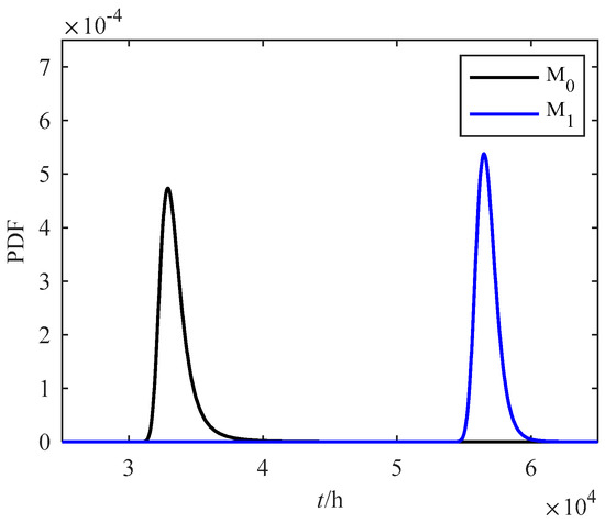
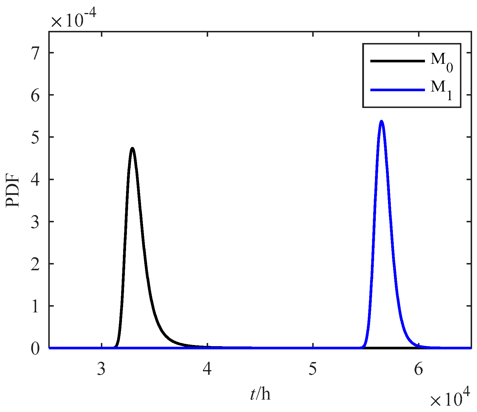
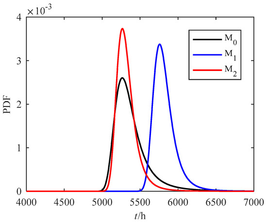
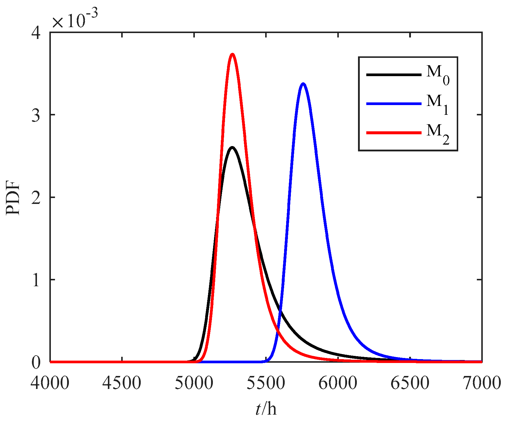
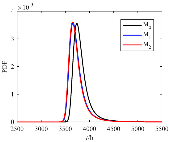
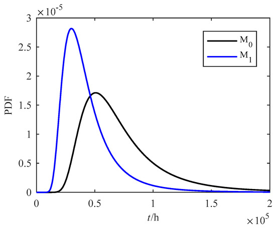
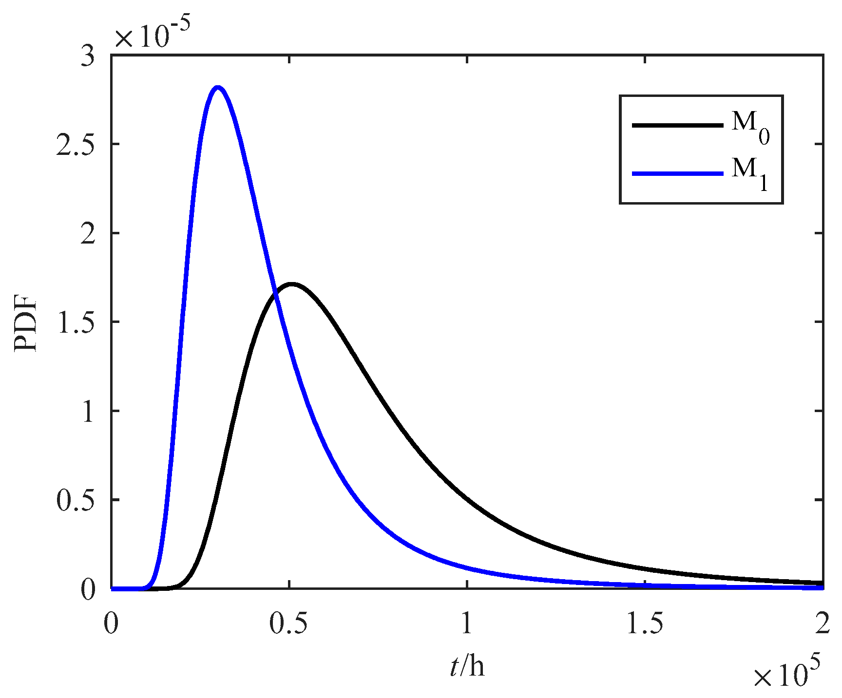
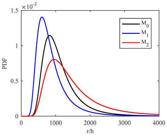
The results obtained in this paper are compared with reference [10]. The distribution parameters of storage lifetime obtained in reference [10] in the normal storage state are also provided in Table 5. The probability density functions of storage lifetimes obtained by the two methods are shown in Figure 1. The model in this paper is denoted by M₀, and the model in the reference [10] is denoted by M₁. As can be seen, the storage lifetimes obtained by the two different methods differ dramatically from each other. In order to analyze causes of the difference, the distribution parameters of storage lifetimes obtained by the two methods at 65 °C, 75 °C, and 85 °C are listed in Table 6, and the failure probability density functions under various accelerated stresses are shown in Figure 2, Figure 3 and Figure 4. As can be seen, the results obtained by the two methods under accelerated stresses have differences.

Figure 1. Comparison of probability density function (PDF) of lifetime at 20 °C for accelerometers.

Table 6. Distribution parameters of lifetime under each accelerated stress based on three methods for accelerometers.

	Temperature	μa	σa2	σB2	b
M0	65 °C	1.7306 × 10−60	7.8608 × 10−121	6.6275 × 10−12	15.438
	75 °C	3.4129 × 10−58	3.2564 × 10−116	2.7474 × 10−11	15.438
	85 °C	5.0105 × 10−56	7.4502 × 10−112	1.0520 × 10−10	15.438
M1	65 °C	1.1670 × 10−67	1.8173 × 10−135	3.6325 × 10−11	17.196
	75 °C	2.5020 × 10−64	2.2892 × 10−128	1.6384 × 10−10	17.196
	85 °C	1.8810 × 10−61	7.1436 × 10−123	2.1433 × 10−10	17.196
M2	65 °C	1.1670 × 10−67	1.8173 × 10−135	3.6325 × 10−11	17.375
	75 °C	2.5020 × 10−64	2.2892 × 10−128	1.6384 × 10−10	17.201
	85 °C	1.8810 × 10−61	7.1436 × 10−123	2.1433 × 10−10	17.012

Figure 2. Comparison of PDF of lifetime at 65 °C for accelerometers.

Figure 3. Comparison of PDF of lifetime at 75 °C for accelerometers.

Figure 4. Comparison of PDF of lifetime at 85 °C for accelerometers.

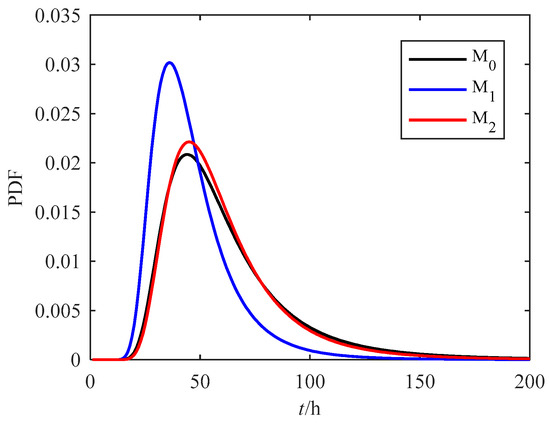
In reference [10], the mean value of time indexes under various accelerated temperature stressesis taken as the time index under the normal temperature stress during extrapolation, while other parameters are kept unchanged. The time index in the distribution parameters of storage lifetime obtained in the reference [10] under various accelerated stresses is replaced with the mean value 17,196, and other parameters are kept unchanged as shown in Table 4 in the reference [10].The degradation parameters under each accelerated stress are estimated by maximum likelihood function where the estimated result is denoted by model M₂. Likewise, the probability density function of M₂ is provided in Figure 2, Figure 3 and Figure 4. The differences between the probability density function of M₁ and those of M₀ and M₂ are very large, indicating that the time index has a great influence on the storage life. When data under accelerated degradation conditions is processed, the time indexes under various temperature stresses cannot be merely averaged. Otherwise the final extrapolated results will be quite different even if the time indexes under various temperature stresses are not significantly different from each other.

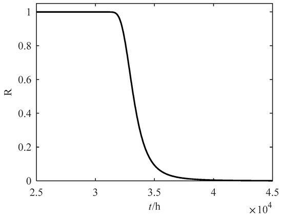
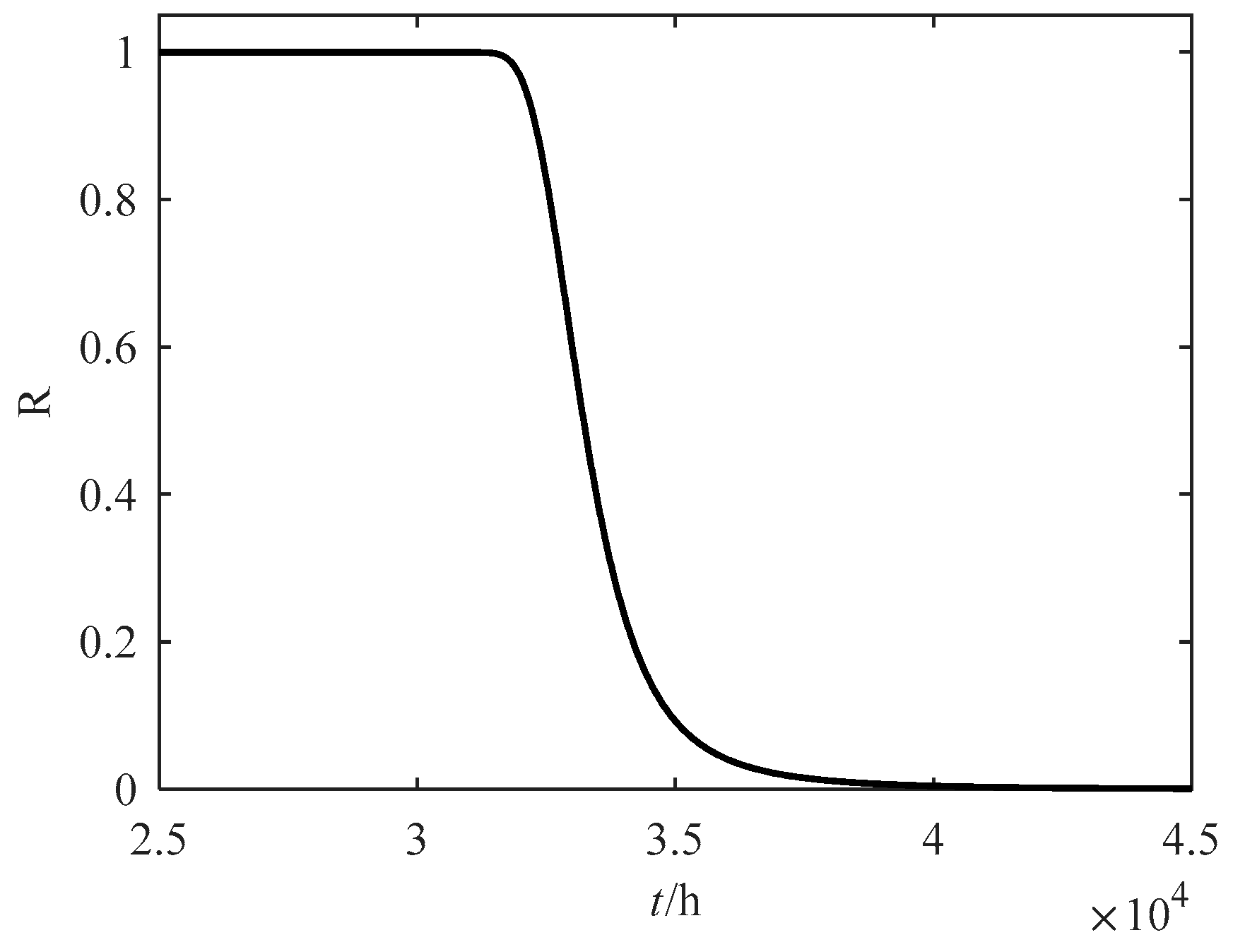
It can be seen from the above analysis that the method provided in this paper is more objective and reasonable, and the impacts of measurement errors are also taken into consideration. The reliability function of storage lifetime under normal storage conditions is shown in Figure 5, and the storage life expectancy thereof is 33,490 h, which is 30,710 h less than 64,200 h obtained in reference [10].

Figure 5. Reliability function of accelerometersat 20 °C.

4.2. O-Type Rubber Sealing Ring

In the fuze system of a certain ammunition, sealing is carried out through an O-type rubber sealing ring, which is necessary in design because of the requirements for reliability and safety in system. Relevant studies show that rubber part is one of the easiest to fail compared with mechanical parts and electronic parts in the ammunition system. In order to obtain the changing rules of the O-type rubber sealing rings quickly, compression permanent deformation rates can be obtained by accelerated degradation tests [20,21]. The data of compression permanent deformation rates of the O-type rubber sealing rings are available in the reference [22]. According to the engineering experience, degradation value y is a function of compression permanent deformation rate as follows.

$$y=-\ln \left(1-\delta \right)$$

where δ means compression permanent deformation rate. When compression permanent deformation rate of O-type rubber sealing ring is great than 31%, air tightness inside the fuze system will be destroyed and the safety will decrease accordingly. So w = 0.3711 is set as the failure threshold of the sealing rings.

Degradation parameters of O-type rubber sealing rings under various accelerated temperature stress levels are estimated through the method in Section 2.1 where the initial values of unknown parameters are introduced in Section 2.2. The estimated parameters are shown in Table 7.

Table 7. Degradation parameters of O-type rubber sealing rings under each accelerated temperature stress.

Temperature	μa	σa2	σB2	σε2	b	lnL
50 ℃	3.306 × 10−2	2.412 × 10−5	9.216 × 10−7	1.870 × 10−5	0.3363	−141.667
60 ℃	4.747 × 10−2	2.201 × 10−5	3.715 × 10−6	6.642 × 10−9	0.3917	−122.118
70 ℃	9.491 × 10−2	1.208 × 10−4	1.081 × 10−5	8.438 × 10−5	0.3396	−118.723
80 ℃	1.243 × 10−1	2.025 × 10−4	2.010 × 10−4	1.339 × 10−9	0.3845	−88.240

Based on the calculation results in Table 7, the estimated values of all degradation parameters in the accelerated degradation model of O-type rubber sealing rings are obtained as shown in Table 8.

Table 8. The estimates of unknown parameters for O-type rubber sealing rings.

α1	α2	α3	β1	β2	β3	b	σε2	lnL
2.081 × 106	2.390 × 109	4.585 × 1022	−5.839 × 103	−1.054 × 104	−2.154 × 104	0.3654	4.919 × 10−5	−456.466

Suppose the temperature stress of O-type rubber seal rings is 25 °C in normal storage environment. The degradation parameters under constant temperature stress can be calculated and obtained as shown in Table 9. Similarly, the degradation parameters under constant temperature stress obtained from model M₁ are also listed in Table 9. Moreover, the probability density functions of lifetime based on these two models are shown in Figure 6.

Table 9. The degradation parameters of O-type rubber sealing rings under 25 °C.

	μa	σa2	σB2	b
M0	6.500 × 10−3	1.049 × 10−6	1.932 × 10−9	0.3654
M1	8.062 × 10−3	1.620 × 10−6	4.247 × 10−9	0.3630

Figure 6. PDF of storage life under 25 °C for O-type rubber seal rings based on of M₀ and M₁.

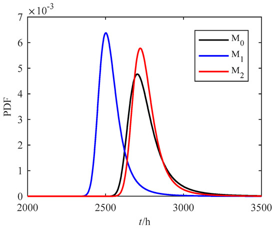
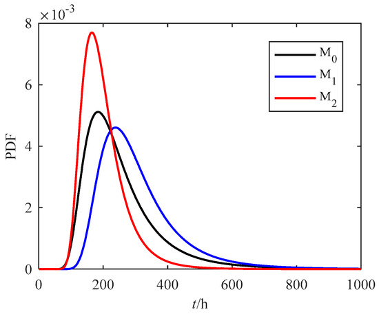
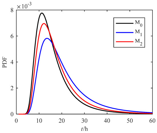
As shown in Figure 6, the probability density functions of lifetime obtained by model M₀ and model M₁ are quite different. In order to analyze the reasons for this phenomenon, the probability density functions under accelerating stresses based on model M₀, model M₁ and model M₂ are given in Figure 7, Figure 8, Figure 9 and Figure 10, The degradation parameters are shown in Table 10.

Figure 7. Comparison of PDF of storage lifetime at 50 °C for O-type rubber seal rings.

Figure 8. Comparison of PDF of storage lifetime at 60 °C for O-type rubber seal rings.

Figure 9. Comparison of PDF of storage lifetime at 70 °C for O-type rubber seal rings.

Figure 10. Comparison of PDF of storage lifetime at 80 °C for O-type rubber seal rings.

Table 10. Distribution parameters of lifetime under each accelerated stress based on three methods for O-type rubber seal rings.

	Temperature	μa	σa2	σB2	b
M0	50 °C	2.957 × 10−2	1.618 × 10−5	5.167 × 10−7	0.3654
	60 °C	5.087 × 10−2	4.308 × 10−5	3.821 × 10−6	0.3654
	70 °C	8.478 × 10−2	1.083 × 10−4	2.515 × 10−5	0.3654
	80 °C	1.373 × 10−1	2.586 × 10−4	1.487 × 10−4	0.3654
M1	50 °C	3.306 × 10−2	2.412 × 10−5	9.216 × 10−7	0.3630
	60 °C	4.747 × 10−2	2.201 × 10−5	3.715 × 10−6	0.3630
	70 °C	9.491 × 10−2	1.208 × 10−4	1.081 × 10−5	0.3630
	80 °C	1.243 × 10−1	2.025 × 10−4	2.010 × 10−4	0.3630
M2	50 °C	3.306 × 10−2	2.412 × 10−5	9.216 × 10−7	0.3363
	60 °C	4.747 × 10−2	2.201 × 10−5	3.715 × 10−6	0.3917
	70 °C	9.491 × 10−2	1.208 × 10−4	1.081 × 10−5	0.3396
	80 °C	1.243 × 10−1	2.025 × 10−4	2.010 × 10−4	0.3845

As can be seen from Figure 7, Figure 8, Figure 9 and Figure 10, it is similar to the accelerometers where the probability density functions of failure lifetime under accelerated stresses obtained from model M₀ and model M₂ are closer compared with the distance of model M₁ and model M₂. It is because the time scale parameters are averaged in model M₁ directly and other parameters remain unchanged. It can be seen that the time index has a great influence on the storage life of O-type rubber seal rings. The conclusion can be derived that the results from the model based on fixed time index presented in this paper are more reasonable.

5. Conclusions

As a key component of the inertial navigation platform of a type of missile, the accelerometer can provide the acceleration information of a moving carrier, and thus quick and accurate estimation of the storage lifetime under normal storage conditions are of great significance. By using the nonlinear Wiener process accelerated degradation model based on a fixed time index proposed in this paper, the obtained storage life expectancy of a certain type of jewel bearing supported pendulous accelerometer is 33,490 h. The comparison and analysis with other models prove that the model obtained in this paper is more consistent with the real situation. Moreover, this method is also applicable to other long-life products with nonlinear degradation characteristics, such as the case study of O-type rubber seal rings. In addition, the results due to model mis-specification and the parameter sensitivity analysis deserve further research.

References

- Deng, A.M.; Chen, X.; Zhang, C.H.; Wang, Y. A comprehensive review of accelerated degradation testing. Acta Armamentarii 2007, 28, 1002–1007. [Google Scholar]
- Escobar, L.A.; Meeker, W.Q. A Review of Accelerated Test Models. Stat. Sci. 2006, 21, 552–577. [Google Scholar] [CrossRef] [Scilit]
- Yuan, X.X.; Pandey, M.D. A nonlinear mixed-effects model for degradation data obtained from in-service inspections. Reliab. Eng. Syst. Saf. 2009, 94, 509–519. [Google Scholar] [CrossRef] [Scilit]
- Tang, S.J.; Guo, X.S.; Yu, C.Q.; Xue, H.J.; Zhou, Z.J. Accelerated degradation tests modeling based on the nonlinear Wiener process with random effects. Math. Probl. Eng. 2014, 2014, 1–11. [Google Scholar] [CrossRef] [Scilit]
- Elsayed, E.A.; Liao, H.T. A geometric Brownian motion model for field degradation data. Int. J. Mater. Prod. Technol. 2004, 20, 51–72. [Google Scholar] [CrossRef] [Scilit]
- Whitmore, G.A.; Schenkelberg, F. Modeling accelerated degradation data using Wiener diffusion with a time scale transformation. Lifetime Data Anal. 1997, 3, 27–45. [Google Scholar] [CrossRef] [Scilit]
- Wang, X.L.; Jiang, P.; Guo, B.; Cheng, Z.J. Real-time reliability evaluation with a general Wiener process-based degradation model. Qual. Reliab. Eng. Int. 2014, 30, 205–220. [Google Scholar] [CrossRef] [Scilit]
- Wang, X.L.; Balakrishnan, N.; Guo, B. Residual life estimation based on a generalized Wiener degradation process. Reliab. Eng. Syst. Saf. 2014, 124, 13–23. [Google Scholar] [CrossRef] [Scilit]
- Si, X.S.; Wang, W.B.; Hu, C.H.; Zhou, D.H.; Pecht, M.G. Remaining useful life estimation based on a nonlinear diffusion degradation process. IEEE Trans. Reliab. 2012, 61, 50–67. [Google Scholar] [CrossRef] [Scilit]
- Li, R.; Wang, L.X.; Gang, L.; Zhou, Z.J.; Automation, D.O. Nonlinear characteristic analysis and storage life forecast for accelerometer based on accelerate degradation model. J. Chin. Inert. Technol. 2014, 22, 125–130. [Google Scholar]
- Whitmore, G.A. Estimating degradation by a Wiener diffusion process subject to measurement error. Lifetime Data Anal. 1995, 1, 307–319. [Google Scholar] [CrossRef] [Scilit]
- Ye, Z.S.; Wang, Y.; Tsui, K.L.; Pecht, M. Degradation data analysis using Wiener processes with measurement errors. IEEE Trans. Reliab. 2013, 62, 772–780. [Google Scholar] [CrossRef] [Scilit]
- Pan, D.H.; Lu, S.L.; Liu, Y.B.; Yang, W.Z.; Liu, J.B. Degradation data analysis using a wiener degradation model with three-source uncertainties. IEEE Access 2019, 7, 37896–37907. [Google Scholar] [CrossRef] [Scilit]
- Li, J.X.; Wang, Z.H.; Zhang, Y.B.; Fu, H.M.; Liu, C.R.; Krishnaswamy, S. Degradation data analysis based on a generalized Wiener process subject to measurement error. Mech. Syst. Signal Process 2017, 94, 57–72. [Google Scholar] [CrossRef] [Scilit]
- Zheng, J.F.; Si, X.S.; Hu, C.H.; Zhang, Z.-X.; Jiang, W. A nonlinear prognostic model for degrading systems with three-source variability. IEEE Trans. Reliab. 2016, 65, 1–15. [Google Scholar] [CrossRef] [Scilit]
- Ye, Z.; Chen, N.; Tsui, K.-L. A Bayesian approach to condition monitoring with imperfect inspections. Qual. Reliab. Eng. Int. 2015, 31, 513–522. [Google Scholar] [CrossRef] [Scilit]
- Li, J.X.; Wang, Z.H.; Liu, X.; Zhang, Y.B.; Fu, H.M.; Liu, C.R. A Wiener process model for accelerated degradation analysis considering measurement errors. Microelectron. Reliab. 2016, 65, 8–15. [Google Scholar] [CrossRef] [Scilit]
- Huang, J.L.; Golubović, D.S.; Koh, S.; Yang, D.G.; Li, X.P.; Fan, X.J.; Zhang, G.Q. Lumen degradation modeling of white-light LEDs in step stress accelerated degradation test. Reliab. Eng. Syst. Saf. 2016, 154, 152–159. [Google Scholar] [CrossRef] [Scilit]
- Ye, Z.S.; Xie, M. Stochastic modelling and analysis of degradation for highly reliable products. Appl. Stoch. Models Bus. Ind. 2015, 31, 16–32. [Google Scholar] [CrossRef] [Scilit]
- El-Hag, A.H.; Jayaram, S.H.; Cherney, E.A. Effect of insulator profile on aging performance of silicone rubber insulators in salt-fog. IEEE Trans. Dielectr. Electr. Insul. 2007, 14, 352–359. [Google Scholar] [CrossRef] [Scilit]
- Woo, C.S.; Choi, S.S.; Lee, S.B.; Kim, H.S. Useful lifetime prediction of rubber components using accelerated testing. IEEE Trans. Reliab. 2010, 59, 11–17. [Google Scholar] [CrossRef] [Scilit]
- Xiao, K.; Gu, X.H.; Peng, C. Reliability Evaluation of the O-type Rubber Sealing Ring for Fuse Based on Constant Stress Accelerated Degradation Testing. J. Mech. Eng. 2014, 50, 62–69. [Google Scholar] [CrossRef] [Scilit]
© 2019 by the authors. Licensee MDPI, Basel, Switzerland. This article is an open access article distributed under the terms and conditions of the Creative Commons Attribution (CC BY) license (http://creativecommons.org/licenses/by/4.0/).