
Overview of Gas Sensors Focusing on Chemoresistive Ones for Cancer Detection


1
Department of Physics and Earth Science, University of Ferrara, 44122 Ferrara, Italy
2
SCENT S.r.l., 44124 Ferrara, Italy
3
Department of Neurosciences and Rehabilitation, University of Ferrara, 44121 Ferrara, Italy
*
Author to whom correspondence should be addressed.
Chemosensors 2023, 11(10), 519; https://doi.org/10.3390/chemosensors11100519
Submission received: 30 August 2023
/
Revised: 20 September 2023
/
Accepted: 29 September 2023
/
Published: 2 October 2023
(This article belongs to the Special Issue An Exciting Journey of Chemical Sensors and Biosensors: A Theme Issue in Honor of Professor Ingemar Lundström)
Abstract
:The necessity of detecting and recognizing gases is crucial in many research and application fields, boosting, in the last years, their continuously evolving technology. The basic detection principle of gas sensors relies on the conversion of gas concentration changes into a readable signal that can be analyzed to calibrate sensors to detect specific gases or mixtures. The large variety of gas sensor types is here examined in detail, along with an accurate description of their fundamental characteristics and functioning principles, classified based on their working mechanisms (electrochemical, resonant, optical, chemoresistive, capacitive, and catalytic). This review is particularly focused on chemoresistive sensors, whose electrical resistance changes because of chemical reactions between the gas and the sensor surface, and, in particular, we focus on the ones developed by us and their applications in the medical field as an example of the technological transfer of this technology to medicine. Nowadays, chemoresistive sensors are, in fact, strong candidates for the implementation of devices for the screening and monitoring of tumors (the second worldwide cause of death, with ~9 million deaths) and other pathologies, with promising future perspectives that are briefly discussed as well.
1. Introduction
The necessity of detecting and recognizing gases is crucial in many research and application fields: industry [1,2,3], environment [4], automotive [3], biomedicine [5,6,7,8], space [9], homeland security [10,11,12], and agri-food [13]. Due to continuously evolving technology and increasing human needs, the growth of the gas sensors market is expected to reach 3 billion USD in 2027, as published in many reports [14,15].
The basic detection principle of gas sensors relies on the conversion of gas concentration changes in the surrounding atmosphere into a readable signal by the transducer that can be analyzed to calibrate sensors to detect specific gases or mixtures. The large variety of gas sensor types is here examined in detail, along with an accurate description of their fundamental characteristics and functioning principles, classified based on their working mechanisms: electrochemical [16], resonant [17], optical [18], chemoresistive (treated here in detail) [19,20], capacitive [21], and catalytic [22].
This review is focused on chemoresistive sensors, whose electrical resistance changes as a result of chemical reactions (reduction or oxidation) between the gas and the active sensor surface. Chemoresistive sensors are based on semiconductor nanostructured films; depending on the film and/or substrate’s physical and geometrical characteristics, they can be classified as: thick-film (with a thickness of tens of µm) [23,24,25], thin-film (with a thickness of 0.1 µm or smaller) [26], or flexible (generally a single or a few sensor material layers on flexible substrates, e.g., to be wearable) [27].
Among the various applications, the progresses of the last decades in the tumor detection field are analyzed here, from the basic research on volatile tumor markers to the realization of oncological screening and monitoring devices based on a core of gas sensors. The focus of this work in the complex panorama of gas sensor technology is exemplified in Figure 1.
Among solid-state semiconductor gas sensors, devices based on semiconductor metal oxide (or metal sulfide) nanostructured films are the most promising, due to their small dimensions, low cost, versatility, high sensitivity (as low as tens of ppb), fast and repeatable responses, portability, low power consumption, cheapness, and easy interfacing with electronic devices [28,29]. After the first observation of the gas-sensing effects in metal-oxide by Seiyama et al. in 1962 [30], these materials began to be widely studied to develop gas sensors. Despite the above-mentioned great advantages, the intrinsic limitation of chemoresistive sensors is their selectivity (i.e., the discrimination capability among different gases), which has, however, been progressively improved thanks to the continuous progress in microelectronic technology and in nanomaterial science. Moreover, to overcome this problem, new sensing materials (with and without doping) have been implemented, as well as grouping different sensors into arrays (i.e., the combination of two or more gas sensors working together). Another important issue is the realization of sensors with highly reproducible responses to meet commercial and industrial requirements [24,31,32]. Reproducibility is indeed fundamental for the application of the same recognition algorithm to different sensors of the same type, guaranteeing univocal results, and being paramount especially in medical screening/monitoring applications. In this respect, this review is centered on the progressive development of suitable materials for biomedical applications and the realization of devices for oncological screening and monitoring (by the detection of tumor volatile biomarkers).
2. Gas Sensors
2.1. Main Sensor Types
A high-performing gas sensor should satisfy the following main requirements:
- -
- High sensitivity (low detection limit of the gas target concentration in the surrounding environment);
- -
- Selectivity (high discrimination power of the gas target from the surrounding atmosphere);
- -
- Repeatability of response in the short, medium, and long term (stability);
- -
- Production reproducibility;
- -
- Cheapness;
- -
- Low power consumption;
- -
- Ease of use;
- -
- Durability;
- -
- Possibility of miniaturization;
- -
- Ease of interfacing with electronic devices.
Among the different gas sensors, the main categories listed in Figure 1 are detailed in this subsection.
Electrochemical gas sensors are devices that are able to determine a target gas concentration by measuring the current resulting from the gas oxidation (or reduction) at an electrode. Electrochemical sensors can be classified into several categories, e.g., amperometric, potentiometric, impedimetric, photoelectrochemical, and electrogenerated chemiluminescent. The operation principle of electrochemical sensors is based on the production of an electrical signal thanks to their reaction with the target analyte. Most of them are amperometric, i.e., capable of generating a current that is linearly proportional to the gas concentration. In practice, the target gas molecules conveyed towards the sensor are first pretreated by an anti-condensation membrane, which also filters dust (Figure 2). Then they diffuse through a capillary, then through a second filter, and finally through a hydrophobic membrane before reaching the sensing electrode surface; the latter is maintained to a fixed voltage, which is applied between the reference electrode and itself. There, the molecules being reduced or oxidized on active catalytic sites acquire or release electrons, thus generating an electric current flowing between the sensing and the counter electrode through the electrolyte filling the cell. This current is conveyed outside the cell through wires terminated with pin connectors, and it is usually measured by means of a potentiostatic circuit [33].
One of the major limitations of electrochemical sensors is the confined temperature range; therefore, they are usually temperature compensated in order to maintain a stable sensor temperature. Another limitation is their short shelf life, typically of six months to one year, and their life span, which could be between one and three years, depending upon their usage and the measured gas type [34].
Another class of gas sensors is the resonant class, consisting of a cantilever that is electrostatically actuated by a couple of electrodes in a resonant mode; the cantilever properties of resonance frequency, vibration amplitude, or quality factor, are measured by means of piezoresistors connected in a Wheatstone bridge configuration (Figure 3). Only the beam tip is coated with a thin layer of a sorbent polymer. The cantilever beam is coated with a chemically sensitive layer, able to adsorb gas molecules from the surrounding atmosphere. Once the gas is adsorbed, the vibrating mass of the cantilever increases, leading to a negative shift in its resonance frequency: the mass resolution of this sensor, working as a microbalance, could be better than 0.4 pg [35,36]. These sensors have been employed to detect humidity, mercury vapors, or a combination of different gases. Sensitive analyte detection in the surrounding atmosphere has been achieved by using a variety of sensing techniques, besides the piezoresistor employment, such as the optical, the mass-sensitive or gravimetric, the calorimetric, and the capacitive techniques.
The main limitation of resonant gas sensors is the progressive resolution decrease as the noise increases. Although the environmental and readout noise can be cancelled or greatly reduced, the thermomechanical noise at finite temperatures, intrinsic to the resonator, cannot be eliminated [37].
Gas concentrations can be easily detected and measured utilizing, for instance, the characteristic optical absorption, emission, or scattering of gas species. By using these physical properties, optical gas sensors have been carefully designed to detect analytes with high sensitivity, specificity, repeatability, and responsivity (even faster than 1 s, allowing in situ, real-time analyte detection). For instance, many gases exhibit high absorption mainly in the ultraviolet–visible (200–400 nm, due to electronic transitions), near-infrared (700 nm to 2.5 μm, due to first harmonic molecular vibrations and rotations), and mid-infrared (2.5–14 μm, due to fundamental molecular vibration and rotation) ranges of the electromagnetic spectrum, with a unique set of absorption bands (Figure 4). Therefore, optical sensors must take advantage of the wavelength and intensity of these bands to be able to detect the analytes and quantify their concentrations [18,38]. Other sensors detect, instead, the fluorescence light emission of the analytes or their light scattering properties, but because of their less common use, they are not reviewed here.
The main limitations of optical sensors are: the interference of ambient light with their operation; the photobleaching or leaching of the indicator, which could impair their long-term stability; and the physical characteristics of the indicator, which limit their dynamic range and selectivity. Finally, the mass transfer of the sample analyte into the indicator phase, which is necessary to obtain an analytical signal, in the end, could contaminate the indicator, compromising its performances [39,40].
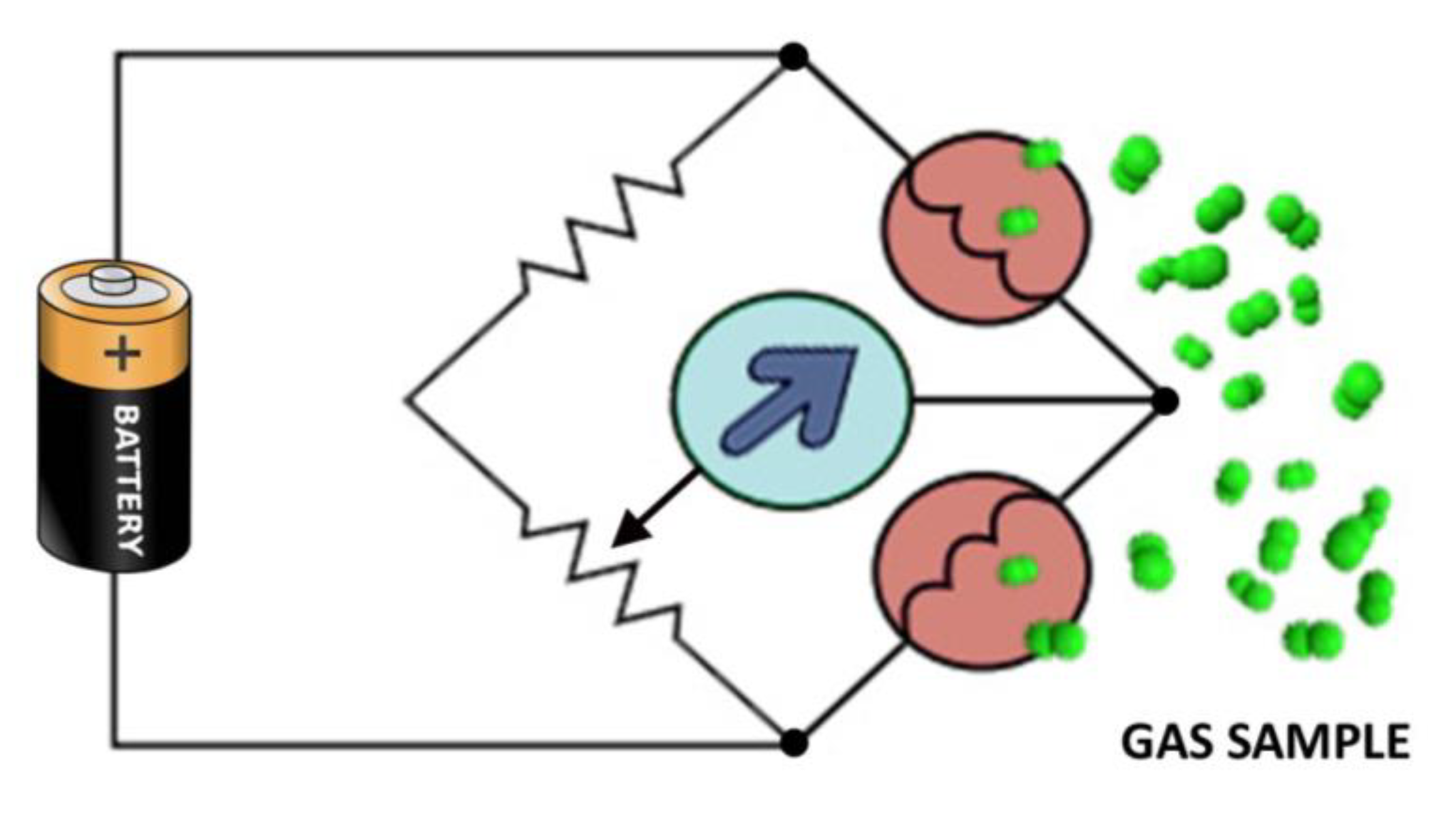
The combustible gases and vapors are mainly detected by catalytic diffusion sensors, usually consisting of two matched “sensing” and “reference” coils: the first one is doped with a catalytic material and is sensitive to combustible gases, the other one is doped with an inert material (i.e., it is “blind” to target gases). A fixed voltage is applied across both coils inserted in a Wheatstone bridge, causing them to heat up to very high temperatures. Combustible gases will burn on the sensing coil only, causing a rise in its temperature and therefore in its resistance, while the temperature and resistance of the reference coil remain unchanged in the presence of the target gases (Figure 5). The bridge is balanced by adjusting a variable resistor (VR) in the presence of clean air. When combustible gases are present, the resistance of the sensing coil will increase, causing an imbalance in the bridge circuit, thus producing an output voltage signal (Vout) which is proportional to the concentration of combustible gases [41].
The main limitation of these sensors is the lack of selectivity towards the flammable gases. Moreover, these sensors could be poisoned by: several elemental organic vapors; some lead compounds (especially tetraethyl lead); sulfur, silicon, and phosphorus compounds; hydrogen sulfide; and halogenated hydrocarbons. Finally, to ensure that combustion happens, the detection environment must contain sufficient oxygen (therefore, they are unable to detect any flammable gas in an oxygen-free environment) [42].
Capacitive type sensors (Figure 6) are able to detect different target gases through the capacitance variations caused by a change in their dielectric constant or a change in their plate thickness induced by the target gas.
Capacitive gas sensors typically detect humidity, CO, hydrocarbons, and CO2: in particular, due to the high water dielectric constant, these sensors are very sensitive to humidity variations because they dramatically change the permittivity of the dielectric material. In particular, the permittivity changes occur in polymers and ceramics, which are the most used material in capacitive type humidity sensors; aluminophosphate-5(AlPO) with pores of uniform size is employed for CO and CO2 detection (the latter is also sensed by 3-amino-propyl-trimethoxysilane and propyl-trimethoxysilane); zeolite is mainly used for hydrocarbon detection. Capacitive sensors also detect analytes by the gas-induced thickness change in their dielectric material, resulting in a change in the electrode distance as well; more rarely, the analyte detection occurs by changing the electrode surface area (as in humidity sensors) [44].
The main limitation of capacitive sensors lies in their high sensitivity to environmental conditions changes (as in humidity, temperature, etc.) and in the complexity of the capacitance measurement with respect to the resistance one. Moreover, the sensor performance can be compromised by the chemical contamination of the polymer composing the dielectric by the sensor hysteresis, which can occur at low temperatures [45].
2.2. Chemoresistive Sensors
Chemoresistive sensors are devices capable of converting an analyte concentration variation into a sensor film resistance change thanks to chemical reactions (reduction and/or oxidation) occurring on the film. For this reason, it is important to maximize the surface-to-volume ratio of the sensing material (e.g., metal oxide or sulfide) by nanostructuring it. These nanostructures can be grown in many different geometries, depending on the specific requirements, such as grains, tubes, sheets, wires, belts, or even more complex ones such as flowers or quantum dots (Figure 7).
Moreover, these nanoshaped films could be manufactured with different thicknesses, usually named “thick” (tens of µm) or “thin” (equal or smaller than 0.1 µm) ones, or printed onto a flexible substrate (to become, for instance, wearable). These semiconductor films are synthesized with different techniques and the most common ones are:
- -
- The hydrothermal method [53], which employs an aqueous solution as a reaction system in a dedicated closed vessel that is heated and pressurized in a controlled mode;
- -
- The “sol-gel” method [54], which involves the conversion of monomers into a colloidal solution (sol) acting as the precursor for an integrated network (gel) of either discrete particles or network polymers; this process has been chosen by the Sensor Laboratory (SL) team of the University of Ferrara for gas sensor production.
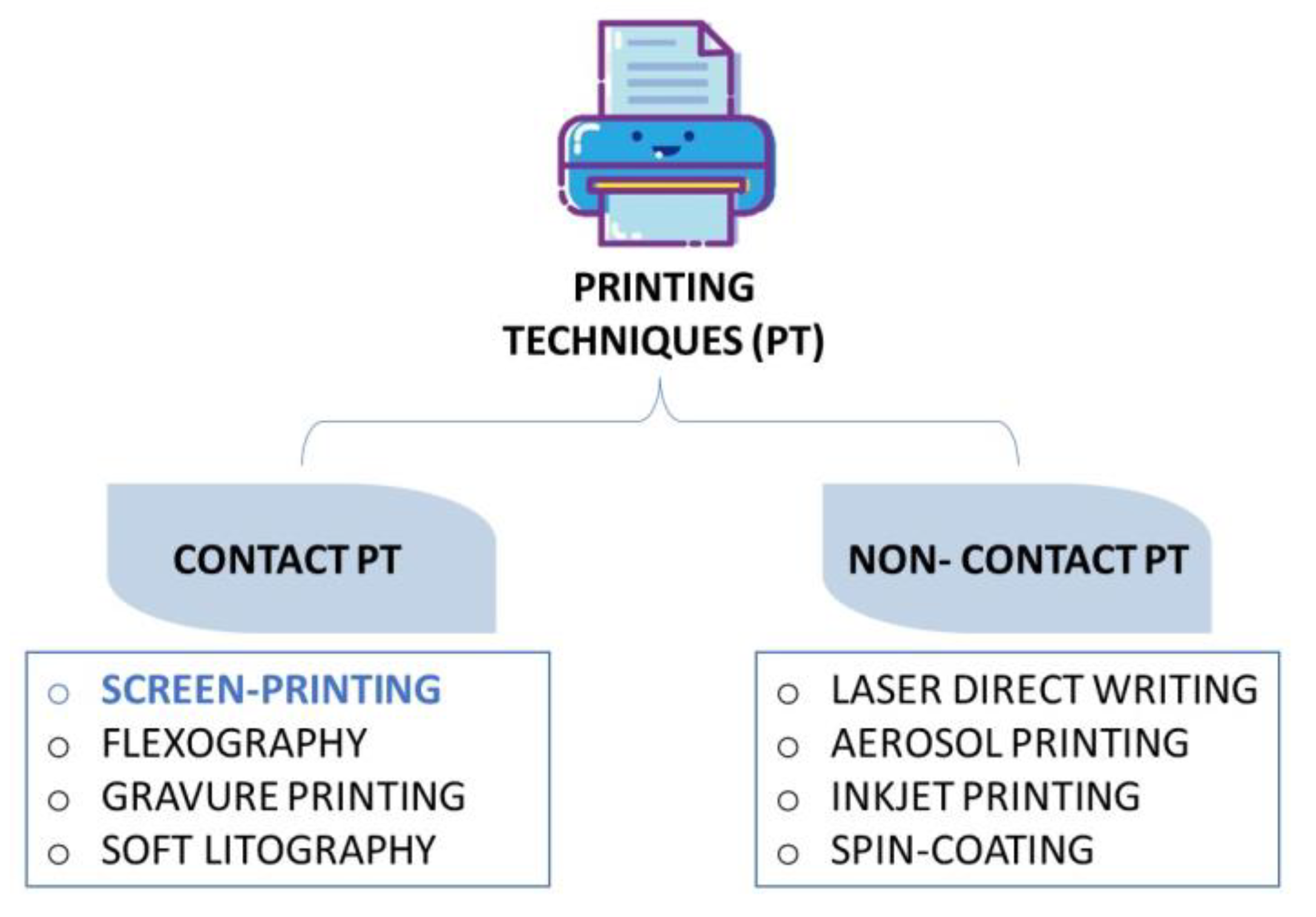
After synthesis, the film is deposited onto a substrate with different technologies depending on the materials employed and the application. These technologies can be divided into contact and non-contact techniques (Figure 8; [55]): contact techniques (e.g., screen-printing, soft lithography, gravure printing, and flexography) involve the printing plate physically touching the substrate; non-contact techniques (e.g., aerosol printing, spin-coating, laser direct writing, and inkjet printing) involve the substrate solely touching the deposition material and not the printing plate. The most widely used technique for sensing film deposition is the serigraphic one [56] (usually by employing a screen-printing machine; Figure 9), in which the semiconductor paste is printed as a film on a substrate (that has the double function of insulator and support), usually made of alumina or silicon.
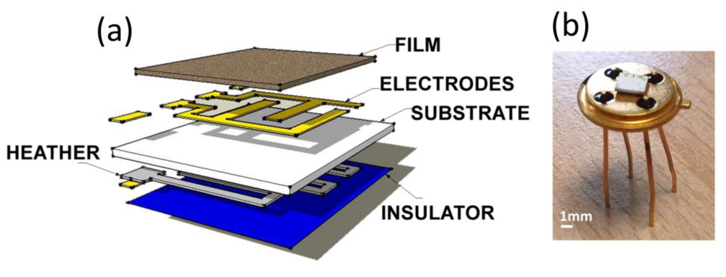
In the case of sensors employed in SL, the film is a square (1 × 1 mm2) of 30 µm thickness, while the alumina substrate is 2.5 × 2.5 mm2.
The substrate hosts, on the front side, two comb-shaped gold electrodes and a heather on the backside (e.g., a platinum meander) to heat the sensor at a desired temperature. Finally, the sensor is bonded with 0.06 mm diameter golden wires by thermocompression onto a TO39 support (by using a bonding machine; Figure 10) [7]. Thermal treatments such as drying (to eliminate volatile organic solvents, usually at 100–150 °C) and firing (to eliminate organic additives and to fix nanostructured dimensions, up to 850 °C), carried out in specific ovens, are fundamental to guarantee sensor stability over time and at high working temperatures (necessary to maximize the thermionic effect but avoid grain coalescence, see below).
Thermal activation is fundamental to activate the sensing film properties and to promote the electrons in the conduction band to create a current among the nanostructures, generated by the potential difference applied between the two electrodes. The working temperatures of a typical metal oxide material range from 300 to 500 °C. However, in those applications in which the sensor cannot be heated at high temperatures, the film activation at room temperature is attained by photoactivation [57] under illumination at specific wavelengths, providing the material with more active sites for gas–surface reactions. Not all the sensing materials can be photoactivated, and only a subclass of semiconductor materials exhibit both chemoresistive and photoconductive properties (e.g., WO3 [58], ZnO [59], CdS [60], and SnS2 [61]).
For the applications treated in this review, the focus is on thick-film sensors made of nanograins, synthesized using the sol–gel technique, then screen-printed and thermally activated. Since the sensing material is a semiconductor, it can be n-type or p-type (depending upon the carrier type: electrons or holes, respectively). Figure 11 represents, schematically, the absorption effect of oxidizing chemical species (atmospheric oxygen) on the semiconductor grain surface. The latter form a region depleted of electrons (depletion region), creating an intergranular potential barrier that electrons must overcome to move from grain to grain, generating a current. This potential barrier is typically parabolic (Figure 11); however, the observed changes in resistance cannot be accounted for solely by thermionic emission because there is also a tunneling contribution [62,63,64]. Therefore, the conductance changes depend not only on the barrier height but also on its width, as tunneling depends on both, and, in general, on the entire barrier shape, which changes as oxygen diffuses into the grain [65].
The conductance of the material depends on the potential barrier height as follows:
where is the bulk conductance ( and have the usual meaning). The interaction of a gaseous species with the oxygen ions occupying the surface states of the sensing material leads to different reaction types that can: (i) release electrons to the conduction band of the material, decreasing the depletion layer width (and so the barrier height and the sensor resistance); (ii) or take electrons from the material bulk, increasing the depletion layer width (and therefore the barrier height and the sensor resistance).
The changes of are detected by an acquisition circuit comprising an operational amplifier in the inverting configuration (Figure 12) in which the sensor is connected to the negative entrance of the amplifier and is polarized by .
The voltage output of the operational amplifier is proportional to the film conductance changes, given by:
where and are the sensor and the feedback resistors. In order to normalize the sensor response to the test gas (labeled as “gas” in Equation (3)) with respect to the baseline acquired in the presence of air only (synthetic or environmental, labeled as “air”), the sensor response is defined as:
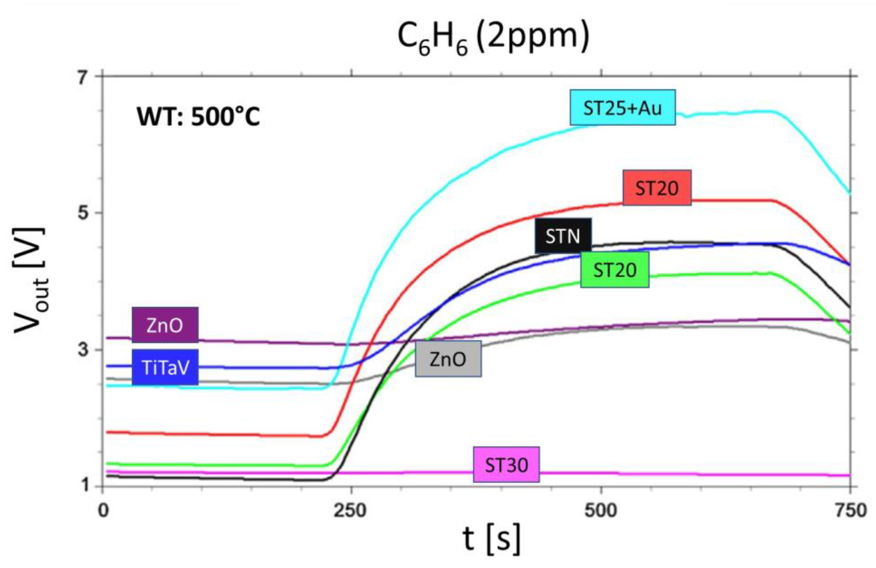
The responses are then analyzed by means of custom algorithms, depending on the study aims (for instance, by using machine learning techniques or a general artificial intelligence algorithm, as in the biomedical applications described below in Chapter 3 [66,67]). Figure 13 shows an example of output voltage curves of eight chemoresistive sensors of different materials in a dry synthetic airflow with benzene at 2 ppm (all the sensors are set at a WT of 500 °C) [68]. Here are visible both the baseline of each sensor and the plateau values, from which the response is calculated by means of Equation (3).
A limitation of chemoresistive sensors is their sensitivity to humidity, which strongly affects their response; therefore, many studies are focused on evaluating humidity interference with target analyte sensing. However, in some studies carried out at SL, it was found that tin oxide-based chemoresistive sensors were able to detect gases such as CO concentrations as low as 1 ppm and at humidity degrees up to 40% with high repeatability [24]. It is possible to conveniently illustrate humidity interference with gas detection by defining a two-dimensional sensitivity, which quantifies the dependence of sensors’ responses to the analyte concentration, the humidity change, and their non-linear combination. The partial derivative of the fitting function with respect to CO concentration not only returns information about the response dependence on the gas concentration, but also on water vapor, even at constant partial pressure, and vice versa [24,25].
3. Main Chemoresistive Sensor Applications
Chemoresistive sensors are very versatile; therefore, they can be employed in a wide range of different applications. One of the main uses of chemoresistive sensors is the detection of air pollutants. The rapid advancements in industrialization have, in fact, led to the release of large amounts of toxic gases into the environment, which have a negative impact both on the planet [69] (e.g., with a decline in plant and animal species diversity [70]) and on human health (e.g., nearly 3.8 million people annually face severe illnesses because of air pollution [71]). Moreover, the presence of sulfur and nitrogen oxides in the atmosphere can cause acid rain and smog that lead to a negative impact on plants and marine organisms [72]. For these reasons, the detection and monitoring of hazardous gases and volatile organic compounds (VOCs) is essential in different working and household environments for promoting occupational and residential health and safety and for protecting the environment. For instance, besides the multitude of toxic gases exhaled by heaters, spray propellants, cleaning products, furniture (such as formaldehyde), glues, etc., at least 420 people die, and more than 100,000 visit the emergency department in the U.S. just from accidental CO poisoning each year [73]. Moreover, the monitoring, through chemoresistive sensors, of the presence of hazardous levels of explosive gases is pivotal in preventing accidents and fire in domestic residences. Moreover, due to their low cost, small size, and ease of use, chemoresistive sensors are also employed in devices for industrial emission control, automotive (e.g., vehicle emission control) and agricultural monitoring, and agri-food processing [74,75,76,77]. Another noticeable application of chemoresistive sensors is in security safeguarding, due to the early and efficient detection of chemical warfare agents (CWAs) that can cause irreversible health damages [12,22]. The last but not least of the main chemoresistive sensor applications is in the biomedical field. In fact, the treatment of diseases at their earliest stages significantly increases survival chances, with additional important savings in treatment costs. The goal of medical diagnostics is to find non-invasive techniques capable of monitoring cancer (e.g., lung cancer, breast cancer, colorectal cancer, etc.) or other diffused pathologies (e.g., diabetes [78], Alzheimer’s [79,80], and Parkinson’s [80]) at their very earliest stages [81]. In the last decades, breath analysis has been one of the most promising candidates [82,83]; in fact, breath can contain volatile biomarkers (e.g., due to metabolic alterations [84]) similar to other human body fluids (e.g., blood, feces, urine, etc.). The use of chemoresistive sensors in specific diagnostic devices will be detailed below.
3.1. Tumor Screening
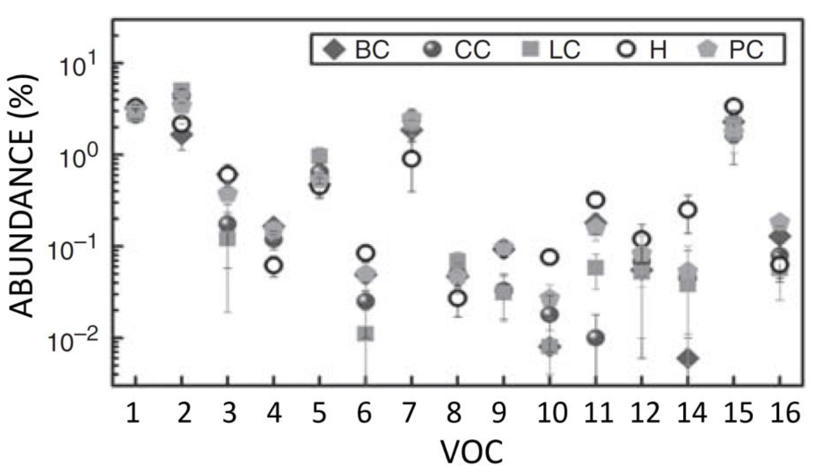
Chemoresistive sensors can offer promising non-invasive (or minimally invasive) methods to identify cancer [6,85,86]. It has been well known since the last decades that volatile organic compound (VOC) emissions, produced by the peroxidation of the cell membrane and alteration of cellular metabolism (for instance, by accelerated glycolysis activity), [87,88,89,90,91,92,93] are strictly related to the presence and growth of a tumor. These VOCs are therefore identified as tumor biomarkers, which can, in principle, be detected both directly (from cancer cells [7,94,95]) and indirectly (e.g., in blood [6,85,91], and from exhaled breath [92,96,97,98,99,100], feces [101,102], urine [103,104], or sweat [105,106]). Vascularized tumor VOCs can, in fact, lead to significant modifications of the blood chemistry, which, in turn, affect the breath composition once the bloodstream reaches the pulmonary alveoli (several VOC concentrations typically range from 20 to 100 ppb [107]). One of the earliest studies performed by Peng et al. [107] on the breath composition with gas chromatography–mass spectrometry (CG-MS) [100,108] identified a pattern of fifteen VOCs of different tumor types (e.g., lung cancer, colon cancer, breast cancer, prostate cancer; Figure 14).
A useful platform cataloguing 450 different VOCs as biomarkers of diverse cancer types, extrapolated from the literature, is the Cancer Odor Database (COD) [109], containing more than 1300 records with 19 critical features for each record, such as the structural and chemical properties (e.g., boiling point, molecular formula, and molecular weight) of VOCs and their origins (as an example, VOCs can be found in breath [110], blood [91], feces [111], urine [112], and sweat [105]). This database is useful for researchers who are developing sensors or electronic nose systems for cancer detection [113] (such as, for instance, a selective chemoresistive sensor for hexanal detection, listed in COD as a biomarker for lung cancer [114]).
Many research studies are focused on the realization of a preventive screening and diagnosis technique for lung cancer through the identification of its biomarkers in breath. This tumor type, in fact, showed over 2.2 million cases and approximately 1.8 million deaths in US, based on the data of “Global Cancer Statistics 2020” on 36 major cancers from 185 countries or regions worldwide [115] and 238,340 cases and 127,070 deaths (see Figure 15 and Table 1) [116,117].
These studies have been focused on the following main goals: the identification of a single VOC as the unique biomarker of lung cancer (such as acetone as an indicator of lung cancer and other illnesses) [118], and the development of medical device prototypes and electronic noses with MOX materials with different structures [119,120], improving their sensitivity and selectivity [121]. However, despite the potential of MOX gas sensors in detecting VOCs in exhaled breath [122,123], there is currently no universal marker for lung cancer [124]. As an example, a set-up based on a ZnO nanosheet chemoresistive sensor, an Arduino system, and a Bluetooth module connected to a smartphone that was realized by Salimi et al. [123] has been conceived to detect VOCs in breath (Figure 16). This device was tested by simulating the breath affected by lung cancer by injecting the biomarkers known from the literature (diethyl ketone, acetone, and isopropanol) [98] into the measurement chamber equipped with the ZnO sensor. These systems, once developed in a functional device, could potentially be used as a non-invasive diagnostic method for lung cancer in its early stage.
Another vehicle of volatile cancer biomarkers can be also human urine, e.g., for the investigation of bladder cancer [125,126], but also, potentially, for other cancer types (e.g., lung, breast, prostate, colorectal, gastric, hepatic, pancreatic, renal, and testicular [103]), as urine is a human body fluid rich in metabolites that easy to handle and available in large amounts without requiring invasive and expensive treatments for collection. Sweat analysis can also be a potential method to detect illnesses by means of the use of specific wearable gas sensors [106]; however, these research studies are still in their preliminary phase and do not lead to any practical results at this time.
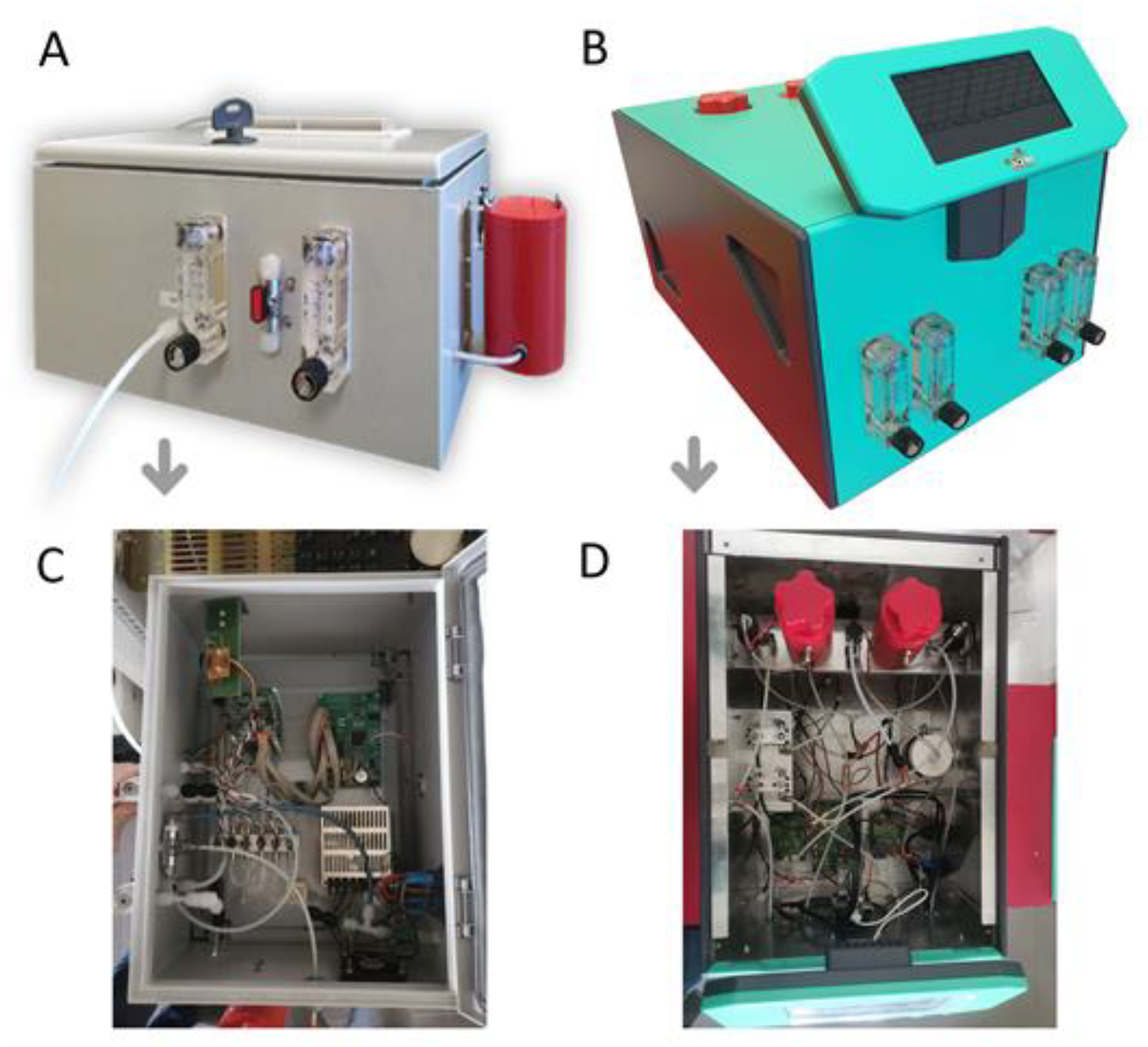
At the SL of UNIFE, a research line aimed at identifying colorectal cancer (CRC) using its biomarkers taken from the literature began in 2013. Colorectal cancer (CRC) has the highest incidence (in both sexes) and the second highest mortality after lung cancer [127], showing 153,020 and 52,550 expected new cases and deaths in 2023 (Table 1 and Figure 15). Nonetheless, if promptly diagnosed, CRC is also one of the most curable cancers (approx. 90% at stage I), and prevention is fundamental to avoid further lesion advancement [128]. A set of different chemoresistive sensor materials, combined into arrays, has been employed in the identification of VOCs listed as CRC-biomarkers in breath (e.g., 1-iodo-nonane [107], decanal [108], and benzene [107] as a representative of VOCs containing benzene rings) in the hypothesis that they may also affect the flatus composition. An artificial intestine has been reproduced in the laboratory [68] by employing a hermetically sealed sensor chamber, a pneumatic system of Teflon tubes, standard gas bottles, and mass flow regulators (controlled by a PC unit running a dedicated software). The sensor responses to the selected CRC-biomarkers were analyzed both singularly and mixed with interferers that are representative digestion products (e.g., H2, CH4, H2S, SO2, N2, NO2, and NO in typical average concentrations [129]) to assess if the chosen arrays are capable of discriminating biomarkers in a normal intestinal atmosphere. It has been demonstrated in other proof of concept studies employing dog smell [130], gas-chromatography, and a commercial electronic nose [101,131], that fecal odor can be altered by CRC volatile emissions. Based on this consideration, the preliminary studies performed at SL paved the way for the implementation of a tailored device for CRC preventive screening through fecal exhalation analysis. The device, named SCENT A1, has been patented in Italy, Germany, and the UK [132], and the first prototype was composed of a microfluidic system, specific electronics, a sensing core with five MOX sensors, and a sensing unit (Figure 17A,C; the basic functioning scheme is reported in Figure 18).
Nowadays, in many countries, the fecal occult blood test (FOBT) is employed in the preventive screening of CRC. As an example, in the Italian region of Emilia-Romagna (as in many other regions of Italy), the Department of Public Health invites all individuals aged between 50 and 69 years to undergo an FIT (the immunochemical version of FOBT) every two years. All FIT positives are subsequently invited to undergo a colonoscopy to further evaluate their health status [86,102]. However, even if FIT is fundamental for prevention, there are many side effects due to the presence of about 65% false positives, inasmuch that the presence of blood in the stool can be due to numerous non-tumor diseases (e.g., inflammatory diseases, diverticula, hemorrhoids, and fissures) [133]. For this reason, a screening method based on the detection of tumor biomarkers, not directly related to occult blood (e.g., VOCs), can be useful to discriminate between CRC false and true positives resulting from FIT. A preliminary study, used to finalize the device, the best sensor array (shown in Table 2), and the analysis protocol, has been performed (in collaboration with the Department of Radiology and Section of General and Thoracic Surgery of the S. Anna Hospital of Ferrara) on fecal samples from CRC-affected patients (extracted during surgery) and from healthy volunteers [134]. As an example, the chosen sensors were successfully able to discriminate the health status of the subjects according to the Principal Component Analysis (PCA; Figure 19). PCA is a multivariate statistical technique that allows to reduction of the data space dimensions without any significant data information loss. It consists of a linear transformation of the original data pool (n-dimensional) (in this case, the sensor responses to each sample exhalations) into a new data pool (n-dimensional), projected in a new Cartesian system in which the data variance is maximized along the main axes (PC1). PC2 is chosen to be perpendicular to PC1, and it is the second axis for variance magnitude. The other axis, containing less and less variance, is often neglected. PCA is useful in those cases in which a system dimensionality reduction is fundamental to improve data visualization as it removes most of the noise and redundancy [135].
On this basis, SCENT A1 and the analysis methods were subjected to a three-year clinical validation protocol (2016–2019), following its approval by the Ethics Committee (number: 151298), involving the following partners from Ferrara: S. Anna Hospital, UNIFE, the Department of Public Health, and SCENT S.r.l. All the participants who had a positive result in the FIT screening program in Ferrara (men and women aged 50–69 who were not CRC diagnosed in the past) were also invited to this experimental trial before colonoscopy investigation (about 1000 subjects). The specificity and sensitivity of this portable device prototype, employing just two selected sensors, resulted in 82.4% and 84.1%, respectively, by means of double-blind tests. The number of sensors was reduced thanks to Support Vector Machine analysis, making the device more easily reproducible and reliable for commercial purposes [86]. This clinical trial was suspended during summer (July and August) to parallel the suspension of the FIT because the chemoresistive sensors do not perform well at high temperatures and humidity and the FIT decreases its specificity in the warmer months [136]. The device was then extensively upgraded in the electronics, pneumatics, packaging (panels B and D of Figure 17), and in the managing software; this strongly improved the user-friendliness of the device, which then obtained CE certification in 2023. The analysis procedure is standardized, simple, and partially automated: firstly, the feces are collected by the patients into a specific standard container and kept in a domestic freezer (−18 °C). The user inserts the defrosted sample in the sample box and starts the measurement by pressing on a virtual button on a touchscreen; the measurements end after about ten minutes giving the result (positive or negative) on the screen by means of an algorithm specifically realized by the SL team, which is able to register and analyze the sensor response curves.
3.2. Tumor Monitoring
Besides the tumor screening, it is important to monitor the health status, the progress of therapeutic pathways, and in general the long-term follow-up of cancer patients. Highly vascularized lesions discharge volatile substances in the bloodstream that could be used as tumor biomarkers; therefore, specific gas sensors, employed in a tailored device, could be successfully devoted to tumor monitoring by sensing the exhalations of human body fluids (such as blood, urine, sweat, etc.). By employing specific sensor arrays, determined by an iterative “trial and error” calibration, it is possible to discriminate tumor-affected patients from healthy subjects by means of two main methods: the identification of a sensor response threshold separating the two classes or with PCA. In the research carried out at the SL and at the Department of Neuroscience and Rehabilitation of UNIFE, a patent prototype (SCENT B1, Figure 20) has been used to perform blood exhalation analysis on tumor-affected patients and on healthy subjects as a control. SCENT B1 [6,8,85] (Figure 20a) comprises a pneumatic system, an electronic unit, and a sensing core. The pneumatic system draws air from the environment and conveys it at a constant pressure, by means of an electronic pump, through a carbon filter (to stabilize the air humidity and temperature) and a 0.2-micron filter (to remove pollutants, such as aerosols, particulate matter, bacteria, and other organic interferers). This clean air flux can be guided directly to the sensors (whose response in this condition is considered the “baseline”, detailed below), or into the sample chamber containing a reusable Teflon container (Figure 20b) filled with a blood sample. The airflow carries the sample headspace VOCs to the sensors by means of a three-way valve. The electronic circuit converts the resistance change of each sensor active film into a voltage that is plotted vs. time by employing a specific software developed by SCENT S.r.l. running on an external PC. The voltage is then transformed into a response R(t) vs. time exploiting Equation (3), which gives results independent of the measured physical quantity and the baseline amplitude, which are generally diverse for each sensor [6,8,85,137].
As an example, the ST25 650 + Au sensor proved to be very effective for tumor marker detection, giving a progressively increasing response with an increase of size and vascularization of the tumor mass and its metastasis (Figure 21). Notably, non-vascularized tumors, not being in contact with the bloodstream, are not detected by the sensor, emphasizing the correlation between the presence of blood tumor markers and sensor response.
Blood samples collected from CRC-affected patients at different stages of their pre- and post-surgery therapeutic path were also analyzed by SCENT B1 to assess its capability of discriminating among these samples. The stages considered were the following ones: T1, the same day of the surgical treatment; T2, before the hospital discharge; T3, after one month from surgery; T4, after 10–12 months from surgery (Figure 22). The four MOX sensors equipping SCENT B1 were all able to discern between T1 and T4, but with different amplitudes (Figure 22a), sensitivities, and specificities (Figure 22b).
The sensor array, composed of these four sensors, resulted in a sensitivity and specificity towards CRC of 93% and 82%, respectively, making the device suitable for patients’ health status monitoring to detect possible post-therapeutic relapses and, more generally, in clinical follow-up protocols.
3.3. Basic Research on Biomarkers
The development of sensors that are more and more specific for CRC detection requires testing them directly on the tumor cell exhalations and on healthy cells as a control. To this aim, the sensor responses to the exhalation of a primary cancer sample and of a healthy sample (both of the same weight, collected during colorectal surgery from the intestine of the same patient, and kept in Dulbecco Modified Eagle Medium, DMEM) were at first statistically analyzed. The employed sensors were: ST25 (based on tin and titanium oxides), STN (based on tin, titanium, and niobium oxides), and TiTaV (based on titanium, tantalum, and vanadium oxides). Preliminary results obtained using PCA indicate that the sensors were able to distinguish between healthy and tumor tissue samples (removed from 13 patients) with coherent responses (the discrimination power of the most sensitive sensor was about 17%), highlighting their strong potential for clinical practice (Figure 23).
This project was further developed to distinguish the VOC patterns of different tumor, immortalized, and healthy cell lines exhalations, by statistically analyzing the sensor responses to them (by employing the same sensors used in the analysis of the explanted tissues described above). The device’s suitability for identifying the cell types and monitoring their growth was determined by analyzing the device output to the VOCs of various cell lines, exhaled at different initial plating concentrations and incubation times. The sensor responses progressively increased along with the cell density and incubation time, except for the sensor W11, which gave unreliable responses to all the tested cell lines (listed in Table 3). All sensors (but W11) gave large and consistent responses to RKO (Figure 24) and HEK293 cells, while they were less responsive to CHO, A549, CACO-2, and fibroblast ones (Figure 25).
The small responses to human skin fibroblasts were expected since they are healthy; therefore, their metabolism is believed to emit VOCs at a lower rate with respect to the cancerous cells (Figure 25, top panel). The CACO-2, derived from human colorectal adenocarcinoma, could also be expected to emit a lower amount of VOCs with respect to more invasive cancer cell lines, as was indeed found (Figure 25, lower panel). Indeed, it is a poorly aggressive tumor, and it has been widely adopted as a model of the intestinal epithelial barrier in order to study the mechanisms implicated in early-stage cancer progression and to test radiation therapeutic efficacy [138].
Figure 25.
Sensor responses to CACO-2 and fibroblast cell lines. Cells plated at 250 K (light colors), 500 K (medium dark colors), and 1 M (darkest colors) cells/dish, measured after being withdrawn from the incubator at 24 h (blue), 48 h (green), and 72 h (orange); cells sorted for the same concentration at different times of incubation. The sensor responses not visible in the histograms were smaller than 0.75. Modified from [95].

Different sensors gave different response amplitudes to the same cell line, while the same sensor gave different response amplitudes to different cell lines [95], illuminating the high potential of MOX sensors to discriminate among various cell types when working inside an array [95]. On this basis, it is possible to construct a matrix that represents the responses of the sensors to different cell lines (with comparable cell densities), so that each set of sensors is able to univocally identify a particular cell line. For example, the entries in this table could be all the sensor responses divided by the response of the less responsive sensor (whose amplitude, reported in red in Table 3, is therefore kept unvaried) to each cell line. W11 was excluded in this computation since it gave unreliable responses.

Table 3.
Responses of ST25, STN, and TiTaV sensors to different cell culture types. W11 was excluded from this computation for its unreliability. Red numbers represent the smallest response given by one of the three sensors to the VOCs exhaled by a particular cell line. Cell cultures analyzed are the following: fibroblasts, human healthy control cells [139]; CACO-2, human colorectal adenocarcinoma cell line; RKO, human colorectal cancer cells; HEK293, specific immortalized cell line originally derived from human embryonic kidney; CHO, epithelial cell line derived from the ovary of the Chinese hamster; A549, explant culture of lung carcinomatous tissue. Modified from [95].
| Cell Type | ST25 | STN | TiTaV |
|---|---|---|---|
| Fibroblasts | 1.11 | 0.78 | 1.17 |
| CACO-2 | 1.03 | 1.00 | 1.14 |
| RKO | 1.14 | 1.29 | 1.01 |
| HEK-293 | 1.12 | 1.12 | 1.15 |
| CHO | 1.08 | 1.33 | 1.20 |
| A549 | 1.35 | 1.06 | 1.30 |
The resulting matrix could be regarded as a “fingerprint response” of the three-sensors array because each cell line is univocally identified by it. The reliability of this strategy depends on the hypothesis that as the cell number increases (but avoiding the cell confluence), the responses of all the sensors increase by the same amount, so that the matrix entries are independent of the number of cells, as, in fact, roughly occurs (Figure 24). To develop a reliable test protocol to discriminate cell cultures by using MOX sensors, it will be paramount to grow three-dimensional cell cultures from healthy and tumor tissues (surgically removed from the same individual). This would allow us to search for the most suitable sensors able to discriminate as well as possible between healthy and tumor tissues (as close as possible to the natural ones) among different cancer types, stages, and grades, and to test the efficacy of antitumor drugs and radiations.
4. Conclusions and Future Perspectives
The present review aimed to present a complete and updated description of the complex gas sensor panorama. The main gas sensor types have been illustrated, along with an accurate description of their fundamental characteristics and functioning principles, focusing on chemoresistive sensors and their applications, and, in particular, in the medical field by the SL of UNIFE. Chemoresistive sensors are, in fact, strong candidates nowadays for the implementation of devices for tumor (and other pathologies) screening and monitoring. The presence of specific biomarkers (correlated to specific pathologies) in human body fluids (e.g., blood, breath, feces, urine, and sweat) is useful for pathology detection. The SL group has developed, in the last years, two main devices: the first one (patented in Italy, Germany, and the UK, clinically validated and CE-certified) is used for colorectal cancer screening by means of fecal exhalations analysis, and the second one (patented in Italy) is used for tumor monitoring through blood exhalations analysis and for basic research on tumor cells. These devices have been described in detail in this review as an example of a strongly transversal technological transfer of gas sensor technology applied to medicine. All the studies could represent a starting point for future research to improve screening and monitoring techniques for cancer detection (being non-invasive or minimally invasive), with great advantages both for population wellbeing and the savings of worldwide Health Services. The basic research on the odor fingerprint of cell cultures (at different tumor stages and grades) could pave the way for different research branches. One of the main future applications could be represented by monitoring the growth of three-dimensional cell lines (derived from surgically removed biopsies), as well as the testing specific drugs before using them on laboratory animals or human test subjects.
5. Patents
- C. Malagù; G. Zonta; S. Gherardi; A. Giberti; N. Landini; A. Gaiardo, Dispositivo per lo screening preliminare di adenomi al colon-retto (2014), National #: RM2014A000595, European #: 3210013 (Germany, UK);
- C. Malagù, S. Gherardi, G. Zonta, N. Landini, A. Giberti, B. Fabbri, A. Gaiardo, G. Anania, G. Rispoli, L. Scagliarini, Combinazione di materiali semiconduttori nanoparticolati per uso nel distinguere cellule normali da cellule tumorali (2015), National #: 102015000057717.
Author Contributions
Conceptualization, writing—original draft preparation, writing—review and editing, supervision, G.Z., G.R., C.M. and M.A. All authors have read and agreed to the published version of the manuscript.
Funding
This research received no external funding.
Institutional Review Board Statement
Not applicable.
Informed Consent Statement
Not applicable.
Data Availability Statement
Not applicable.
Acknowledgments
This research has been supported and partially funded by the Italian Ministero dell’ Università e della Ricerca (PRIN 20228AAJRL, PRIN 2017KC8WMB).
Conflicts of Interest
The authors declare no conflict of interest.
References
- Shu, L.; Mukherjee, M.; Wu, X. Toxic Gas Boundary Area Detection in Large-Scale Petrochemical Plants with Industrial Wireless Sensor Networks. IEEE Commun. Mag. 2016, 54, 22–28. [Google Scholar] [CrossRef]
- Spector, Y.; Jacobson, E. Novel Technology for Flame & Gas Detection in the Petrochemical Industry. In Proceedings of the International Petroleum Conference and Exhibition of Mexico, Villahermosa, Mexico, 3–5 March 1998. [Google Scholar]
- Velasco, G.; Schnell, J.-P. Gas Sensors and Their Applications in the Automotive Industry. J. Phys. 1983, 16, 973. [Google Scholar] [CrossRef]
- Martinelli, G.; Carotta, M.C.; Ferroni, M.; Sadaoka, Y.; Traversa, E. Screen-Printed Perovskite-Type Thick Films as Gas Sensors for Environmental Monitoring. Sens. Actuators B Chem. 1999, 55, 99–110. [Google Scholar] [CrossRef]
- Sakumura, Y.; Koyama, Y.; Tokutake, H.; Hida, T.; Sato, K.; Itoh, T.; Akamatsu, T.; Shin, W. Diagnosis by Volatile Organic Compounds in Exhaled Breath from Lung Cancer Patients Using Support Vector Machine Algorithm. Sensors 2017, 17, 287. [Google Scholar] [CrossRef] [PubMed]
- Astolfi, M.; Rispoli, G.; Anania, G.; Artioli, E.; Nevoso, V.; Zonta, G.; Malagù, C. Tin, Titanium, Tantalum, Vanadium and Niobium Oxide Based Sensors to Detect Colorectal Cancer Exhalations in Blood Samples. Molecules 2021, 26, 466. [Google Scholar] [CrossRef] [PubMed]
- Astolfi, M.; Rispoli, G.; Anania, G.; Nevoso, V.; Artioli, E.; Landini, N.; Benedusi, M.; Melloni, E.; Secchiero, P.; Tisato, V.; et al. Colorectal Cancer Study with Nanostructured Sensors: Tumor Marker Screening of Patient Biopsies. Nanomaterials 2020, 10, E606. [Google Scholar] [CrossRef] [PubMed]
- Landini, N.; Anania, G.; Astolfi, M.; Fabbri, B.; Guidi, V.; Rispoli, G.; Valt, M.; Zonta, G.; Malagù, C. Nanostructured Chemoresistive Sensors for Oncological Screening and Tumor Markers Tracking: Single Sensor Approach Applications on Human Blood and Cell Samples. Sensors 2020, 20, 1411. [Google Scholar] [CrossRef] [PubMed]
- Hunter, G.W.; Chen, L.-Y.; Neudeck, P.G.; Knight, D.; Liu, C.-C.; Wu, Q.-H.; Zhou, H.-J. Chemical Gas Sensors for Aeronautic and Space Applications; NASA: Boston, MA, USA, 1997. [Google Scholar]
- Potyrailo, R.A.; Morris, W.G. Multianalyte Chemical Identification and Quantitation Using a Single Radio Frequency Identification Sensor. Anal. Chem. 2007, 79, 45–51. [Google Scholar] [CrossRef]
- Potyrailo, R.A.; Nagraj, N.; Surman, C.; Boudries, H.; Lai, H.; Slocik, J.M.; Kelley-Loughnane, N.; Naik, R.R. Wireless Sensors and Sensor Networks for Homeland Security Applications. TrAC Trends Anal. Chem. 2012, 40, 133–145. [Google Scholar] [CrossRef]
- Barreca, D.; Maccato, C.; Gasparotto, A. Metal Oxide Nanosystems As Chemoresistive Gas Sensors for Chemical Warfare Agents: A Focused Review. Adv. Mater. Interfaces 2022, 9, 2102525. [Google Scholar] [CrossRef]
- Love, C.; Nazemi, H.; El-Masri, E.; Ambrose, K.; Freund, M.S.; Emadi, A. A Review on Advanced Sensing Materials for Agricultural Gas Sensors. Sensors 2021, 21, 3423. [Google Scholar] [CrossRef] [PubMed]
- Chansin, G.; Pugh, D. Environmental Gas Sensors 2017–2027; CISION: Cambridge, UK, 2016. [Google Scholar]
- Reportlinker Environmental Gas Sensors 2017–2027. Available online: https://www.prnewswire.com/news-releases/environmental-gas-sensors-2017-2027-300377842.html (accessed on 24 July 2023).
- Ruiz Simões, F.; Xavier, M.G. Electrochemical Sensors. In Nanoscience and Its Applications; William Andrew: Norwich, NY, USA, 2017; pp. 155–178. ISBN 978-0-323-49780-0. [Google Scholar]
- Aloisio, D.; Donato, N. Development of Gas Sensors on Microstrip Disk Resonators. Procedia Eng. 2014, 87, 1083–1086. [Google Scholar] [CrossRef]
- Hodgkinson, J.; Tatam, R.P. Optical Gas Sensing: A Review. Meas. Sci. Technol. 2013, 24, 012004. [Google Scholar] [CrossRef]
- Franco, M.A.; Conti, P.P.; Andre, R.S.; Correa, D.S. A Review on Chemiresistive ZnO Gas Sensors. Sens. Actuators Rep. 2022, 4, 100100. [Google Scholar] [CrossRef]
- Velmathi, G.; Mohan, S.; Henry, R. Analysis and Review of Tin Oxide-Based Chemoresistive Gas Sensor. IETE Tech. Rev. 2016, 33, 323–331. [Google Scholar] [CrossRef]
- Arena, A.; Donato, N.; Saitta, G. Capacitive Humidity Sensors Based on MWCNTs/Polyelectrolyte Interfaces Deposited on Flexible Substrates. Microelectron. J. 2009, 40, 887–890. [Google Scholar] [CrossRef]
- Lee, E.-B.; Hwang, I.-S.; Cha, J.-H.; Lee, H.-J.; Lee, W.-B.; Pak, J.J.; Lee, J.-H.; Ju, B.-K. Micromachined Catalytic Combustible Hydrogen Gas Sensor. Sens. Actuators B Chem. 2011, 153, 392–397. [Google Scholar] [CrossRef]
- Bârsan, N.; Weimar, U. Understanding the Fundamental Principles of Metal Oxide Based Gas Sensors; the Example of CO Sensing with SnO2 Sensors in the Presence of Humidity. J. Phys. Condens. Matter 2003, 15, R813. [Google Scholar] [CrossRef]
- Astolfi, M.; Rispoli, G.; Gherardi, S.; Zonta, G.; Malagù, C. Reproducibility and Repeatability Tests on (SnTiNb)O2 Sensors in Detecting ppm-Concentrations of CO and Up to 40% of Humidity: A Statistical Approach. Sensors 2023, 23, 1983. [Google Scholar] [CrossRef]
- Gherardi, S.; Zonta, G.; Astolfi, M.; Malagù, C. Humidity Effects on SnO2 and (SnTiNb)O2 Sensors Response to CO and Two-Dimensional Calibration Treatment. Mater. Sci. Eng. B 2021, 265, 115013. [Google Scholar] [CrossRef]
- Parellada-Monreal, L.; Gherardi, S.; Zonta, G.; Malagù, C.; Casotti, D.; Cruciani, G.; Guidi, V.; Martínez-Calderón, M.; Castro-Hurtado, I.; Gamarra, D.; et al. WO3 Processed by Direct Laser Interference Patterning for NO2 Detection. Sens. Actuators B Chem. 2020, 305, 127226. [Google Scholar] [CrossRef]
- Alvarado, M.; La Flor, S.D.; Llobet, E.; Romero, A.; Ramírez, J.L. Performance of Flexible Chemoresistive Gas Sensors after Having Undergone Automated Bending Tests. Sensors 2019, 19, 5190. [Google Scholar] [CrossRef] [PubMed]
- Comini, E.; Faglia, G.; Sberveglieri, G.; Pan, Z.; Wang, Z.L. Stable and Highly Sensitive Gas Sensors Based on Semiconducting Oxide Nanobelts. Appl. Phys. Lett. 2002, 81, 1869–1871. [Google Scholar] [CrossRef]
- Wang, C.; Yin, L.; Zhang, L.; Xiang, D.; Gao, R. Metal Oxide Gas Sensors: Sensitivity and Influencing Factors. Sensors 2010, 10, 2088–2106. [Google Scholar] [CrossRef] [PubMed]
- Seiyama, T.; Kato, A.; Fujiishi, K.; Nagatani, M. A New Detector for Gaseous Components Using Semiconductive Thin Films. Anal. Chem. 1962, 34, 1502–1503. [Google Scholar] [CrossRef]
- Yamazoe, N. Toward Innovations of Gas Sensor Technology. Sens. Actuators B Chem. 2005, 108, 2–14. [Google Scholar] [CrossRef]
- Zonta, G.; Astolfi, M.; Casotti, D.; Cruciani, G.; Fabbri, B.; Gaiardo, A.; Gherardi, S.; Guidi, V.; Landini, N.; Valt, M.; et al. Reproducibility Tests with Zinc Oxide Thick-Film Sensors. Ceram. Int. 2019, 46. [Google Scholar] [CrossRef]
- Electrochemical Gas Sensors—Membrapor. Available online: https://www.membrapor.ch/electrochemical-gas-sensors/ (accessed on 24 July 2023).
- Panjan, P.; Ohtonen, E.; Tervo, P.; Virtanen, V.; Sesay, A.M. Shelf Life of Enzymatic Electrochemical Sensors. Procedia Technol. 2017, 27, 306–308. [Google Scholar] [CrossRef]
- Lange, D.; Brand, O.; Baltes, H. Resonant Gas Sensor. In CMOS Cantilever Sensor Systems: Atomic Force Microscopy and Gas Sensing Applications; Lange, D., Brand, O., Baltes, H., Eds.; Microtechnology and Mems; Springer: Berlin/Heidelberg, Germany, 2002; pp. 57–83. ISBN 978-3-662-05060-6. [Google Scholar]
- Hajjaj, A.Z.; Jaber, N.; Alcheikh, N.; Younis, M.I. A Resonant Gas Sensor Based on Multimode Excitation of a Buckled Microbeam. IEEE Sens. J. 2020, 20, 1778–1785. [Google Scholar] [CrossRef]
- Manzaneque, T.; Ghatkesar, M.K.; Alijani, F.; Xu, M.; Norte, R.A.; Steeneken, P.G. Resolution Limits of Resonant Sensors. Phys. Rev. Appl. 2023, 19, 054074. [Google Scholar] [CrossRef]
- Mishra, V.; Rashmi; Sukriti. Optical Gas Sensors; IntechOpen: London, UK, 2022; ISBN 978-1-80356-962-8. [Google Scholar]
- Wang, W. Advances in Chemical Sensors; IntechOpen: London, UK, 2012; ISBN 978-953-307-792-5. [Google Scholar]
- Pizzoferrato, R. Optical Chemical Sensors: Design and Applications. Sensors 2023, 23, 5284. [Google Scholar] [CrossRef] [PubMed]
- Catalytic Type—Operating Principle—Technology—FIGARO Engineering Inc. Available online: https://www.figaro.co.jp/en/technicalinfo/principle/catalytic-type.html (accessed on 24 July 2023).
- Principles, Advantages and Disadvantages of Common Sensors of Gas Detectors. Available online: https://www.aiyitec.com/info/principles-advantages-and-disadvantages-of-co-46102599.html (accessed on 19 September 2023).
- Ahmad, W.R.W.; Mamat, M.H.; Zoolfakar, A.S.; Khusaimi, Z.; Rusop, M. A Review on Hematite α-Fe2O3 Focusing on Nanostructures, Synthesis Methods and Applications. In Proceedings of the 2016 IEEE Student Conference on Research and Development (SCOReD), Kuala Lumpur, Malaysia, 13–14 December 2016; pp. 1–6. [Google Scholar]
- Ishihara, T.; Matsubara, S. Capacitive Type Gas Sensors. J. Electroceramics 1998, 2, 215–228. [Google Scholar] [CrossRef]
- Prior, E.M.; Brumbelow, K.; Miller, G.R. Measurement of Above-Canopy Meteorological Profiles Using Unmanned Aerial Systems. Hydrol. Process. 2020, 34, 865–867. [Google Scholar] [CrossRef]
- Bargougui, R.; Omri, K.; Mhemdi, A.; Ammar, S. Synthesis and Characterization of SnO2 Nanoparticles: Effect of Hydrolysis Rate on the Optical Properties. Adv. Mater. Lett. 2015, 6, 816–819. [Google Scholar] [CrossRef]
- Liu, Y.; Jiao, Y.; Qu, F.; Gong, L.; Wu, X. Facile Synthesis of Template-Induced SnO2 Nanotubes. J. Nanomater. 2013, 2013, e610964. [Google Scholar] [CrossRef]
- Park, M.-S.; Wang, G.-X.; Kang, Y.-M.; Wexler, D.; Dou, S.-X.; Liu, H.-K. Preparation and Electrochemical Properties of SnO2 Nanowires for Application in Lithium-Ion Batteries. Angew. Chem. 2007, 119, 764–767. [Google Scholar] [CrossRef]
- Choi, P.G.; Izu, N.; Shirahata, N.; Masuda, Y. SnO2 Nanosheets for Selective Alkene Gas Sensing. ACS Appl. Nano Mater. 2019, 2, 1820–1827. [Google Scholar] [CrossRef]
- Liu, Y.; Huang, J.; Yang, J.; Wang, S. Pt Nanoparticles Functionalized 3D SnO2 Nanoflowers for Gas Sensor Application. Solid-State Electron. 2017, 130, 20–27. [Google Scholar] [CrossRef]
- Zou, R.; Hu, J.; Zhang, Z.; Chen, Z.; Liao, M. SnO2 Nanoribbons: Excellent Field-Emitters. CrystEngComm 2011, 13, 2289–2293. [Google Scholar] [CrossRef]
- Lu, X.; Wang, H.; Wang, Z.; Jiang, Y.; Cao, D.; Yang, G. Room-Temperature Synthesis of Colloidal SnO2 Quantum Dot Solution and Ex-Situ Deposition on Carbon Nanotubes as Anode Materials for Lithium Ion Batteries. J. Alloys Compd. 2016, 680, 109–115. [Google Scholar] [CrossRef]
- Fan, H.; Zheng, X.; Shen, Q.; Wang, W.; Dong, W. Hydrothermal Synthesis and Their Ethanol Gas Sensing Performance of 3-Dimensional Hierarchical Nano Pt/SnO2. J. Alloys Compd. 2022, 909, 164693. [Google Scholar] [CrossRef]
- Bokov, D.; Turki Jalil, A.; Chupradit, S.; Suksatan, W.; Javed Ansari, M.; Shewael, I.H.; Valiev, G.H.; Kianfar, E. Nanomaterial by Sol-Gel Method: Synthesis and Application. Adv. Mater. Sci. Eng. 2021, 2021, e5102014. [Google Scholar] [CrossRef]
- Cruz, S.; Rocha, L.; Viana, J. Printing Technologies on Flexible Substrates for Printed Electronics; IntechOpen: London, UK, 2018; ISBN 978-1-78923-456-5. [Google Scholar]
- Simonenko, N.P.; Fisenko, N.A.; Fedorov, F.S.; Simonenko, T.L.; Mokrushin, A.S.; Simonenko, E.P.; Korotcenkov, G.; Sysoev, V.V.; Sevastyanov, V.G.; Kuznetsov, N.T. Printing Technologies as an Emerging Approach in Gas Sensors: Survey of Literature. Sensors 2022, 22, 3473. [Google Scholar] [CrossRef] [PubMed]
- Kumar, R.; Liu, X.; Zhang, J.; Kumar, M. Room-Temperature Gas Sensors Under Photoactivation: From Metal Oxides to 2D Materials. Nano-Micro Lett. 2020, 12, 164. [Google Scholar] [CrossRef] [PubMed]
- Imran, M.; Rashid, S.S.A.A.H.; Sabri, Y.; Motta, N.; Tesfamichael, T.; Sonar, P.; Shafiei, M. Template Based Sintering of WO3 Nanoparticles into Porous Tungsten Oxide Nanofibers for Acetone Sensing Applications. J. Mater. Chem. C 2019, 7, 2961–2970. [Google Scholar] [CrossRef]
- Espid, E.; Adeli, B.; Taghipour, F. Enhanced Gas Sensing Performance of Photo-Activated, Pt-Decorated, Single-Crystal ZnO Nanowires. J. Electrochem. Soc. 2019, 166, H3223. [Google Scholar] [CrossRef]
- Giberti, A.; Casotti, D.; Cruciani, G.; Fabbri, B.; Gaiardo, A.; Guidi, V.; Malagù, C.; Zonta, G.; Gherardi, S. Electrical Conductivity of CdS Films for Gas Sensing: Selectivity Properties to Alcoholic Chains. Sens. Actuators B Chem. 2015, 207, 504–510. [Google Scholar] [CrossRef]
- Gaiardo, A.; Fabbri, B.; Guidi, V.; Bellutti, P.; Giberti, A.; Gherardi, S.; Vanzetti, L.; Malagù, C.; Zonta, G. Metal Sulfides as Sensing Materials for Chemoresistive Gas Sensors. Sensors 2016, 16, 296. [Google Scholar] [CrossRef]
- Castro, M.S.; Aldao, C.M. Prebreakdown Conduction in Zinc Oxide Varistors: Thermionic or Tunnel Currents and One-step or Two-step Conduction Processes. Appl. Phys. Lett. 1993, 63, 1077–1079. [Google Scholar] [CrossRef]
- Blaustein, G.; Castro, M.S.; Aldao, C.M. Influence of Frozen Distributions of Oxygen Vacancies on Tin Oxide Conductance. Sens. Actuators B Chem. 1999, 55, 33–37. [Google Scholar] [CrossRef]
- Aldao, C.M.; Mirabella, D.A.; Ponce, M.A.; Giberti, A.; Malagù, C. Role of Intragrain Oxygen Diffusion in Polycrystalline Tin Oxide Conductivity. J. Appl. Phys. 2011, 109, 063723. [Google Scholar] [CrossRef]
- Aldao, C.M.; Malagù, C. Non-Parabolic Intergranular Barriers in Tin Oxide and Gas Sensing. J. Appl. Phys. 2012, 112, 024518. [Google Scholar] [CrossRef]
- Aharon, M.; Elad, M.; Bruckstein, A. K-SVD: An Algorithm for Designing Overcomplete Dictionaries for Sparse Representation. IEEE Trans. Signal Process. 2006, 54, 4311–4322. [Google Scholar] [CrossRef]
- Zonta, G.; Astolfi, M.; de Togni, A.; Gaiardo, A.; Gherardi, S.; Guidi, V.; Landini, N.; Palmonari, C.; Malagù, C. Sensing Device for Colorectal Cancer Preventive Screening through Fecal Odor Analysis: Clinical Validation Outcomes. ECS Meet. Abstr. 2020, MA2020-01, 2032. [Google Scholar] [CrossRef]
- Zonta, G.; Fabbri, B.; Giberti, A.; Guidi, V.; Landini, N.; Malagù, C. Detection of Colorectal Cancer Biomarkers in the Presence of Interfering Gases. Procedia Eng. 2014, 87, 596–599. [Google Scholar] [CrossRef]
- Calderón-Garcidueñas, L.; Mora-Tiscareño, A.; Ontiveros, E.; Gómez-Garza, G.; Barragán-Mejía, G.; Broadway, J.; Chapman, S.; Valencia-Salazar, G.; Jewells, V.; Maronpot, R.R.; et al. Air Pollution, Cognitive Deficits and Brain Abnormalities: A Pilot Study with Children and Dogs. Brain Cogn. 2008, 68, 117–127. [Google Scholar] [CrossRef] [PubMed]
- Therivel, J.G.; Therivel, R. Introduction to Environmental Impact Assessment, 5th ed.; Routledge: London, UK, 2019; ISBN 978-0-429-47073-8. [Google Scholar]
- Schraufnagel, D.E.; Balmes, J.R.; Cowl, C.T.; De Matteis, S.; Jung, S.-H.; Mortimer, K.; Perez-Padilla, R.; Rice, M.B.; Riojas-Rodriguez, H.; Sood, A.; et al. Air Pollution and Noncommunicable Diseases: A Review by the Forum of International Respiratory Societies’ Environmental Committee, Part 2: Air Pollution and Organ Systems. Chest 2019, 155, 417–426. [Google Scholar] [CrossRef]
- Manisalidis, I.; Stavropoulou, E.; Stavropoulos, A.; Bezirtzoglou, E. Environmental and Health Impacts of Air Pollution: A Review. Front. Public Health 2020, 8, 14. [Google Scholar] [CrossRef]
- Carbon Monoxide. Available online: https://www.cdc.gov/nceh/features/copoisoning/index.html (accessed on 25 July 2023).
- Gaiardo, A.; Krik, S.; Valt, M.; Fabbri, B.; Tonezzer, M.; Feng, Z.; Guidi, V.; Bellutti, P. Development of a Sensor Array Based on Pt, Pd, Ag and Au Nanocluster Decorated SnO2 for Precision Agriculture. ECS Meet. Abstr. 2021, MA2021-01, 1550. [Google Scholar] [CrossRef]
- Gallardo, A.H. Hydrogeological Characterisation and Groundwater Exploration for the Development of Irrigated Agriculture in the West Kimberley Region, Western Australia. Groundw. Sustain. Dev. 2019, 8, 187–197. [Google Scholar] [CrossRef]
- Strati, V.; Albéri, M.; Anconelli, S.; Baldoncini, M.; Bittelli, M.; Bottardi, C.; Chiarelli, E.; Fabbri, B.; Guidi, V.; Raptis, K.G.C.; et al. Modelling Soil Water Content in a Tomato Field: Proximal Gamma Ray Spectroscopy and Soil–Crop System Models. Agriculture 2018, 8, 60. [Google Scholar] [CrossRef]
- Neethirajan, S.; Jayas, D.S.; Sadistap, S. Carbon Dioxide (CO2) Sensors for the Agri-Food Industry—A Review. Food Bioprocess Technol. 2009, 2, 115–121. [Google Scholar] [CrossRef]
- Ochoa-Muñoz, Y.H.; Mejía de Gutiérrez, R.; Rodríguez-Páez, J.E. Metal Oxide Gas Sensors to Study Acetone Detection Considering Their Potential in the Diagnosis of Diabetes: A Review. Molecules 2023, 28, 1150. [Google Scholar] [CrossRef] [PubMed]
- Mazzatenta, A.; Pokorski, M.; Sartucci, F.; Domenici, L.; Di Giulio, C. Volatile Organic Compounds (VOCs) Fingerprint of Alzheimer’s Disease. Respir. Physiol. Neurobiol. 2015, 209, 81–84. [Google Scholar] [CrossRef] [PubMed]
- Tisch, U.; Schlesinger, I.; Ionescu, R.; Nassar, M.; Axelrod, N.; Robertman, D.; Tessler, Y.; Azar, F.; Marmur, A.; Aharon-Peretz, J.; et al. Detection of Alzheimer’s and Parkinson’s Disease from Exhaled Breath Using Nanomaterial-Based Sensors. Nanomedicine 2013, 8, 43–56. [Google Scholar] [CrossRef] [PubMed]
- Nasiri, N.; Clarke, C. Nanostructured Chemiresistive Gas Sensors for Medical Applications. Sensors 2019, 19, 462. [Google Scholar] [CrossRef] [PubMed]
- Moon, H.G.; Jung, Y.; Han, S.D.; Shim, Y.-S.; Jung, W.-S.; Lee, T.; Lee, S.; Park, J.H.; Baek, S.-H.; Kim, J.-S.; et al. All Villi-like Metal Oxide Nanostructures-Based Chemiresistive Electronic Nose for an Exhaled Breath Analyzer. Sens. Actuators B Chem. 2018, 257, 295–302. [Google Scholar] [CrossRef]
- Aasi, A.; Aghaei, S.M.; Panchapakesan, B. Noble Metal (Pt or Pd)-Decorated Atomically Thin MoS2 as a Promising Material for Sensing Colorectal Cancer Biomarkers through Exhaled Breath. Int. J. Comput. Mater. Sci. Eng. 2024, 13, 2350014. [Google Scholar] [CrossRef]
- Hammoudi, N.; Ahmed, K.B.R.; Garcia-Prieto, C.; Huang, P. Metabolic Alterations in Cancer Cells and Therapeutic Implications. Chin. J. Cancer 2011, 30, 508–525. [Google Scholar] [CrossRef]
- Astolfi, M.; Rispoli, G.; Anania, G.; Zonta, G.; Malagù, C. Chemoresistive Nanosensors Employed to Detect Blood Tumor Markers in Patients Affected by Colorectal Cancer in a One-Year Follow Up. Cancers 2023, 15, 1797. [Google Scholar] [CrossRef]
- Zonta, G.; Malagù, C.; Gherardi, S.; Giberti, A.; Pezzoli, A.; De Togni, A.; Palmonari, C. Clinical Validation Results of an Innovative Non-Invasive Device for Colorectal Cancer Preventive Screening through Fecal Exhalation Analysis. Cancers 2020, 12, 1471. [Google Scholar] [CrossRef] [PubMed]
- Jang, M.; Kim, S.S.; Lee, J. Cancer Cell Metabolism: Implications for Therapeutic Targets. Exp. Mol. Med. 2013, 45, e45. [Google Scholar] [CrossRef] [PubMed]
- Van der Paal, J.; Neyts, E.C.; Verlackt, C.C.W.; Bogaerts, A. Effect of Lipid Peroxidation on Membrane Permeability of Cancer and Normal Cells Subjected to Oxidative Stress. Chem. Sci. 2016, 7, 489–498. [Google Scholar] [CrossRef] [PubMed]
- Masotti, L.; Casali, E.; Gesmundo, N.; Sartor, G.; Galeotti, T.; Borrello, S.; Piretti, M.V.; Pagliuca, G. Lipid Peroxidation in Cancer Cells: Chemical and Physical Studies. Ann. N. Y. Acad. Sci. 1988, 551, 47–57; discussion 57–58. [Google Scholar] [CrossRef] [PubMed]
- Schmidt, K.; Podmore, I. Current Challenges in Volatile Organic Compounds Analysis as Potential Biomarkers of Cancer. J. Biomark. 2015, 2015, 981458. [Google Scholar] [CrossRef] [PubMed]
- Wang, C.; Li, P.; Lian, A.; Sun, B.; Wang, X.; Guo, L.; Chi, C.; Liu, S.; Zhao, W.; Luo, S.; et al. Blood Volatile Compounds as Biomarkers for Colorectal Cancer. Cancer Biol. Ther. 2014, 15, 200–206. [Google Scholar] [CrossRef] [PubMed]
- Amann, A.; Mochalski, P.; Ruzsanyi, V.; Broza, Y.Y.; Haick, H. Assessment of the Exhalation Kinetics of Volatile Cancer Biomarkers Based on Their Physicochemical Properties. J. Breath Res. 2014, 8, 016003. [Google Scholar] [CrossRef]
- Bratulic, S.; Limeta, A.; Dabestani, S.; Birgisson, H.; Enblad, G.; Stålberg, K.; Hesselager, G.; Häggman, M.; Höglund, M.; Simonson, O.E.; et al. Noninvasive Detection of Any-Stage Cancer Using Free Glycosaminoglycans. Proc. Natl. Acad. Sci. USA 2022, 119, e2115328119. [Google Scholar] [CrossRef]
- Bajaj, J.S.; Saeian, K.; Schubert, C.M.; Hafeezullah, M.; Franco, J.; Varma, R.R.; Gibson, D.P.; Hoffmann, R.G.; Stravitz, R.T.; Heuman, D.M.; et al. Minimal Hepatic Encephalopathy Is Associated with Motor Vehicle Crashes: The Reality beyond the Driving Test. Hepatology 2009, 50, 1175–1183. [Google Scholar] [CrossRef]
- Astolfi, M.; Rispoli, G.; Benedusi, M.; Zonta, G.; Landini, N.; Valacchi, G.; Malagù, C. Chemoresistive Sensors for Cellular Type Discrimination Based on Their Exhalations. Nanomaterials 2022, 12, 1111. [Google Scholar] [CrossRef]
- Ligor, M.; Ligor, T.; Bajtarevic, A.; Ager, C.; Pienz, M.; Klieber, M.; Denz, H.; Fiegl, M.; Hilbe, W.; Weiss, W.; et al. Determination of Volatile Organic Compounds in Exhaled Breath of Patients with Lung Cancer Using Solid Phase Microextraction and Gas Chromatography Mass Spectrometry. Clin. Chem. Lab. Med. 2009, 47, 550–560. [Google Scholar] [CrossRef] [PubMed]
- Mazzone, P.J. Analysis of Volatile Organic Compounds in the Exhaled Breath for the Diagnosis of Lung Cancer. J. Thorac. Oncol. 2008, 3, 774–780. [Google Scholar] [CrossRef] [PubMed]
- Bajtarevic, A.; Ager, C.; Pienz, M.; Klieber, M.; Schwarz, K.; Ligor, M.; Ligor, T.; Filipiak, W.; Denz, H.; Fiegl, M.; et al. Noninvasive Detection of Lung Cancer by Analysis of Exhaled Breath. BMC Cancer 2009, 9, 348. [Google Scholar] [CrossRef] [PubMed]
- Horvath, E.; Majlis, S.; Rossi, R.; Franco, C.; Niedmann, J.P.; Castro, A.; Dominguez, M. An Ultrasonogram Reporting System for Thyroid Nodules Stratifying Cancer Risk for Clinical Management. J. Clin. Endocrinol. Metab. 2009, 94, 1748–1751. [Google Scholar] [CrossRef] [PubMed]
- Altomare, D.F.; Di Lena, M.; Porcelli, F.; Trizio, L.; Travaglio, E.; Tutino, M.; Dragonieri, S.; Memeo, V.; de Gennaro, G. Exhaled Volatile Organic Compounds Identify Patients with Colorectal Cancer. Br. J. Surg. 2013, 100, 144–150. [Google Scholar] [CrossRef]
- de Meij, T.G.; Larbi, I.B.; van der Schee, M.P.; Lentferink, Y.E.; Paff, T.; Terhaar Sive Droste, J.S.; Mulder, C.J.; van Bodegraven, A.A.; de Boer, N.K. Electronic Nose Can Discriminate Colorectal Carcinoma and Advanced Adenomas by Fecal Volatile Biomarker Analysis: Proof of Principle Study. Int. J. Cancer 2014, 134, 1132–1138. [Google Scholar] [CrossRef] [PubMed]
- Zonta, G.; Anania, G.; Astolfi, M.; Feo, C.; Gaiardo, A.; Gherardi, S.; Alessio, G.; Guidi, V.; Landini, N.; Palmonari, C.; et al. Chemoresistive Sensors for Colorectal Cancer Preventive Screening through Fecal Odor: Double-Blind Approach. Sens. Actuators B Chem. 2019, 301, 127062. [Google Scholar] [CrossRef]
- Bax, C.; Lotesoriere, B.J.; Sironi, S.; Capelli, L. Review and Comparison of Cancer Biomarker Trends in Urine as a Basis for New Diagnostic Pathways. Cancers 2019, 11, 1244. [Google Scholar] [CrossRef]
- Chandrapalan, S.; Arasaradnam, R.P. Urine as a Biological Modality for Colorectal Cancer Detection. Expert Rev. Mol. Diagn. 2020, 20, 489–496. [Google Scholar] [CrossRef]
- Monedeiro, F.; Dos Reis, R.B.; Peria, F.M.; Sares, C.T.G.; De Martinis, B.S. Investigation of Sweat VOC Profiles in Assessment of Cancer Biomarkers Using HS-GC-MS. J. Breath Res. 2020, 14, 026009. [Google Scholar] [CrossRef]
- Gao, F.; Liu, C.; Zhang, L.; Liu, T.; Wang, Z.; Song, Z.; Cai, H.; Fang, Z.; Chen, J.; Wang, J.; et al. Wearable and Flexible Electrochemical Sensors for Sweat Analysis: A Review. Microsyst. Nanoeng. 2023, 9, 1. [Google Scholar] [CrossRef] [PubMed]
- Peng, G.; Hakim, M.; Broza, Y.Y.; Billan, S.; Abdah-Bortnyak, R.; Kuten, A.; Tisch, U.; Haick, H. Detection of Lung, Breast, Colorectal, and Prostate Cancers from Exhaled Breath Using a Single Array of Nanosensors. Br. J. Cancer 2010, 103, 542–551. [Google Scholar] [CrossRef] [PubMed]
- Di Lena, M.; Porcelli, F.; Altomare, D.F. Volatile Organic Compounds as New Biomarkers for Colorectal Cancer: A Review. Color. Dis. 2016, 18, 654–663. [Google Scholar] [CrossRef] [PubMed]
- COD. Available online: http://bioinf.modares.ac.ir/software/COD/ (accessed on 24 July 2023).
- Phillips, M.; Gleeson, K.; Hughes, J.M.; Greenberg, J.; Cataneo, R.N.; Baker, L.; McVay, W.P. Volatile Organic Compounds in Breath as Markers of Lung Cancer: A Cross-Sectional Study. Lancet 1999, 353, 1930–1933. [Google Scholar] [CrossRef] [PubMed]
- Bond, A.; Greenwood, R.; Lewis, S.; Corfe, B.; Sarkar, S.; O’Toole, P.; Rooney, P.; Burkitt, M.; Hold, G.; Probert, C. Volatile Organic Compounds Emitted from Faeces as a Biomarker for Colorectal Cancer. Aliment. Pharmacol. Ther. 2019, 49, 1005–1012. [Google Scholar] [CrossRef] [PubMed]
- da Costa, B.R.B.; De Martinis, B.S. Analysis of Urinary VOCs Using Mass Spectrometric Methods to Diagnose Cancer: A Review. Clin. Mass Spectrom. 2020, 18, 27–37. [Google Scholar] [CrossRef]
- Janfaza, S.; Banan Nojavani, M.; Khorsand, B.; Nikkhah, M.; Zahiri, J. Cancer Odor Database (COD): A Critical Databank for Cancer Diagnosis Research. Database 2017, 2017, bax055. [Google Scholar] [CrossRef]
- Janfaza, S.; Banan Nojavani, M.; Nikkhah, M.; Alizadeh, T.; Esfandiar, A.; Ganjali, M.R. A Selective Chemiresistive Sensor for the Cancer-Related Volatile Organic Compound Hexanal by Using Molecularly Imprinted Polymers and Multiwalled Carbon Nanotubes. Microchim. Acta 2019, 186, 137. [Google Scholar] [CrossRef]
- Sung, H.; Ferlay, J.; Siegel, R.L.; Laversanne, M.; Soerjomataram, I.; Jemal, A.; Bray, F. Global Cancer Statistics 2020: GLOBOCAN Estimates of Incidence and Mortality Worldwide for 36 Cancers in 185 Countries. CA Cancer J. Clin. 2021, 71, 209–249. [Google Scholar] [CrossRef]
- Common Cancer Types—NCI. Available online: https://www.cancer.gov/types/common-cancers (accessed on 24 July 2023).
- Siegel, R.L.; Miller, K.D.; Wagle, N.S.; Jemal, A. Cancer Statistics, 2023. CA Cancer J. Clin. 2023, 73, 17–48. [Google Scholar] [CrossRef]
- Ahmadipour, M.; Pang, A.L.; Ardani, M.R.; Pung, S.-Y.; Ooi, P.C.; Hamzah, A.A.; Mohd Razip Wee, M.F.; Aniq Shazni Mohammad Haniff, M.; Dee, C.F.; Mahmoudi, E.; et al. Detection of Breath Acetone by Semiconductor Metal Oxide Nanostructures-Based Gas Sensors: A Review. Mater. Sci. Semicond. Process. 2022, 149, 106897. [Google Scholar] [CrossRef]
- Borowik, P.; Adamowicz, L.; Tarakowski, R.; Wacławik, P.; Oszako, T.; Ślusarski, S.; Tkaczyk, M. Development of a Low-Cost Electronic Nose for Detection of Pathogenic Fungi and Applying It to Fusarium Oxysporum and Rhizoctonia Solani. Sensors 2021, 21, 5868. [Google Scholar] [CrossRef] [PubMed]
- Yuan, H.; Li, N.; Fan, W.; Cai, H.; Zhao, D. Metal-Organic Framework Based Gas Sensors. Adv. Sci. 2022, 9, 2104374. [Google Scholar] [CrossRef]
- Vajhadin, F.; Mazloum-Ardakani, M.; Amini, A. Metal Oxide-Based Gas Sensors for the Detection of Exhaled Breath Markers. Med. Devices Sens. 2021, 4, e10161. [Google Scholar] [CrossRef] [PubMed]
- Peled, N.; Hakim, M.; Bunn, P.A.; Miller, Y.E.; Kennedy, T.C.; Mattei, J.; Mitchell, J.D.; Hirsch, F.R.; Haick, H. Non-Invasive Breath Analysis of Pulmonary Nodules. J. Thorac. Oncol. 2012, 7, 1528–1533. [Google Scholar] [CrossRef] [PubMed]
- Salimi, M.; Milani Hosseini, S.M.R. Smartphone-Based Detection of Lung Cancer-Related Volatile Organic Compounds (VOCs) Using Rapid Synthesized ZnO Nanosheet. Sens. Actuators B Chem. 2021, 344, 130127. [Google Scholar] [CrossRef]
- Li, G.; Zhu, X.; Liu, J.; Li, S.; Liu, X. Metal Oxide Semiconductor Gas Sensors for Lung Cancer Diagnosis. Chemosensors 2023, 11, 251. [Google Scholar] [CrossRef]
- Lett, L.; George, M.; Slater, R.; De Lacy Costello, B.; Ratcliffe, N.; García-Fiñana, M.; Lazarowicz, H.; Probert, C. Investigation of Urinary Volatile Organic Compounds as Novel Diagnostic and Surveillance Biomarkers of Bladder Cancer. Br. J. Cancer 2022, 127, 329–336. [Google Scholar] [CrossRef]
- Pinto, J.; Carapito, Â.; Amaro, F.; Lima, A.R.; Carvalho-Maia, C.; Martins, M.C.; Jerónimo, C.; Henrique, R.; de Lourdes Bastos, M.; de Pinho, P.G. Discovery of Volatile Biomarkers for Bladder Cancer Detection and Staging through Urine Metabolomics. Metabolites 2021, 11, 199. [Google Scholar] [CrossRef]
- Colorectal Cancer Statistics|How Common Is Colorectal Cancer? Available online: https://www.cancer.org/cancer/types/colon-rectal-cancer/about/key-statistics.html (accessed on 24 July 2023).
- Cancer of the Colon and Rectum—Cancer Stat Facts. Available online: https://seer.cancer.gov/statfacts/html/colorect.html (accessed on 24 July 2023).
- Tomlin, J.; Lowis, C.; Read, N.W. Investigation of Normal Flatus Production in Healthy Volunteers. Gut 1991, 32, 665–669. [Google Scholar] [CrossRef]
- Sonoda, H.; Kohnoe, S.; Yamazato, T.; Satoh, Y.; Morizono, G.; Shikata, K.; Morita, M.; Watanabe, A.; Morita, M.; Kakeji, Y.; et al. Colorectal Cancer Screening with Odour Material by Canine Scent Detection. Gut 2011, 60, 814–819. [Google Scholar] [CrossRef] [PubMed]
- Zhang, Y.; Lorenzi, M.F.; Goddard, K.; Spinelli, J.J.; Gotay, C.; McBride, M.L. Late Morbidity Leading to Hospitalization among 5-Year Survivors of Young Adult Cancer: A Report of the Childhood, Adolescent and Young Adult Cancer Survivors Research Program. Int. J. Cancer 2014, 134, 1174–1182. [Google Scholar] [CrossRef] [PubMed]
- Malagù, C.; Gherardi, S.; Zonta, G.; Landini, N.; Giberti, A.; Fabbri, B.; Gaiardo, A.; Anania, G.; Rispoli, G.; Scagliarini, L. Combinazione Di Materiali Semiconduttori Nanoparticolati per Uso Nel Distinguere Cellule Normali Da Cellule Tumorali. Italian Patent 102015000057717, 10 February 2015. [Google Scholar]
- Allison, J.E.; Fraser, C.G.; Halloran, S.P.; Young, G.P. Population Screening for Colorectal Cancer Means Getting FIT: The Past, Present, and Future of Colorectal Cancer Screening Using the Fecal Immunochemical Test for Hemoglobin (FIT). Gut Liver 2014, 8, 117–130. [Google Scholar] [CrossRef] [PubMed]
- Zonta, G.; Anania, G.; de Togni, A.; Gaiardo, A.; Gherardi, S.; Giberti, A.; Guidi, V.; Landini, N.; Palmonari, C.; Ricci, L.; et al. Use of Gas Sensors and FOBT for the Early Detection of Colorectal Cancer. Proceedings 2017, 1, 398. [Google Scholar] [CrossRef]
- Jolliffe, I.T.; Cadima, J. Principal Component Analysis: A Review and Recent Developments. Philos. Trans. R. Soc. A 2016, 374, 20150202. [Google Scholar] [CrossRef]
- Grazzini, G.; Ventura, L.; Zappa, M.; Ciatto, S.; Confortini, M.; Rapi, S.; Rubeca, T.; Visioli, C.B.; Halloran, S.P. Influence of Seasonal Variations in Ambient Temperatures on Performance of Immunochemical Faecal Occult Blood Test for Colorectal Cancer Screening: Observational Study from the Florence District. Gut 2010, 59, 1511–1515. [Google Scholar] [CrossRef] [PubMed]
- Astolfi, M.; Zonta, G.; Landini, N.; Gherardi, S.; Rispoli, G.; Anania, G.; Benedusi, M.; Guidi, V.; Palmonari, C.; Secchiero, P. Chemoresistive Nanostructured Sensors for Tumor Pre-Screening. Multidiscip. Digit. Publ. Inst. Proc. 2019, 14, 29. [Google Scholar]
- Guardamagna, I.; Lonati, L.; Savio, M.; Stivala, L.A.; Ottolenghi, A.; Baiocco, G. An Integrated Analysis of the Response of Colorectal Adenocarcinoma Caco-2 Cells to X-ray Exposure. Front. Oncol. 2021, 11, 688919. [Google Scholar] [CrossRef]
- Sticozzi, C.; Belmonte, G.; Pecorelli, A.; Cervellati, F.; Leoncini, S.; Signorini, C.; Ciccoli, L.; De Felice, C.; Hayek, J.; Valacchi, G. Scavenger Receptor B1 Post-Translational Modifications in Rett Syndrome. FEBS Lett. 2013, 587, 2199–2204. [Google Scholar] [CrossRef]
Figure 1.
Scheme of gas sensor technology panorama. This review is focused on the tumor detection biomedical application of thick-film chemoresistive gas sensors.
Figure 1.
Scheme of gas sensor technology panorama. This review is focused on the tumor detection biomedical application of thick-film chemoresistive gas sensors.

Figure 2.
Scheme of an electrochemical sensor. Modified from [33].
Figure 2.
Scheme of an electrochemical sensor. Modified from [33].

Figure 3.
Sketch of a cantilever beam gas sensor. Electrodes (in green in panel (a)) are used for the electrostatic actuation of the beam (in pink in panels (a,b)), while the piezoresistor transduces the cantilever movement into an electrical signal (panel (b)); the heater is sketched in blue.
Figure 3.
Sketch of a cantilever beam gas sensor. Electrodes (in green in panel (a)) are used for the electrostatic actuation of the beam (in pink in panels (a,b)), while the piezoresistor transduces the cantilever movement into an electrical signal (panel (b)); the heater is sketched in blue.

Figure 4.
Sketch of a typical optical gas sensor. (a) Global view of the sensing apparatus, comprising a light emitter (usually a laser beam or an LED, sketched with the light bulb), a chamber in which the gas (blue spheres) is fluxed, and a detector, endowed with a light filter to select the desired wavelength; (b) maximal sensor signal (shown by the sketched meter) in the presence of low gas concentration (a few blue spheres) with the light emitter on (red light bulb); (c) lower sensor signal in the presence of higher gas concentration, (d) sensor signal in the absence of light (grey bulb).

Figure 5.
Sketch of a typical catalytic gas sensor inserted into a Wheatstone bridge. The green spheres represent the target gas; the pink coils are the “sensing” and “reference” ones; the light blue circle with the arrow represents the voltage meter; the variable resistance balances the Wheatstone bridge.

Figure 6.
Sketch of a typical capacitive gas sensor, with an expanded view of its interior. Modified from [43].
Figure 6.
Sketch of a typical capacitive gas sensor, with an expanded view of its interior. Modified from [43].

Figure 7.
Main chemoresistive sensor nanostructures. All the SEM images are taken from SnO2 sensor films published in different papers; modified from [28,46,47,48,48,49,50,51,52].

Figure 8.
Scheme of printing technologies. The technique employed by SL is in blue.

Figure 9.
Scheme of the screen-printing process.

Figure 10.
Typical structure of a chemoresistive gas sensor. (a) The layers composing the sensor; (b) photograph of the assembled sensor on a TO39 support.
Figure 10.
Typical structure of a chemoresistive gas sensor. (a) The layers composing the sensor; (b) photograph of the assembled sensor on a TO39 support.

Figure 11.
Sketch of the conduction mechanism between nanograins. Top, two grains are schematically represented with their structure composed of a bulk at the center (in pink), the depletion region (in yellow), and the surface occupied by oxygen ions; bottom, the level of the potential barriers between grains is indicated by the dashed line.

Figure 12.
Inverting operational amplifier.

Figure 13.
Example of sensor output voltage curves to 2 ppm C6H6. (measured in Volts) is plotted vs. time (measured in seconds); the sensors are all heated at a WT of 500 °C and are: ST25 + Au (mixture of tin and titanium oxide at 25% with addition of gold nanoparticles); two ST20 (mixture of tin and titanium oxide at 20%); STN (mixture of tin, titanium, and niobium oxide); ST30 (mixture of tin and titanium oxide at 20%); two ZnO (zin oxide); and TiTaV (solid solution of titanium oxide with addition of tantalum and vanadium). Modified from [68].

Figure 14.
Breath VOC patterns of different tumor types obtained with GC-MS. Fifteen VOCs that are biomarkers for breast (BC), colorectal (CC), lung (LC), and prostate (PC) cancers compared with healthy controls (H). GC-MS analysis did not yield compounds without overlap in abundance for lung cancer, breast cancer, colorectal cancer, and prostate cancer and healthy test groups together. The VOCs were tentatively identified as: VOC 1 ¼ 1-methyl-4-(1-methylethyl)benzene (m/z ¼ 119; CAS: 99-87-6); VOC 2 ¼ toluene (m/z ¼ 91; CAS: 108-88-3); VOC 3 ¼ dodecane (m/z ¼ 57; CAS: 112-40-3); VOC 4 ¼ 3,3-dimethyl pentane (m/z ¼ 43; CAS: 562-49-2); VOC 5 ¼ 2,3,4-trimethyl hexane (m/z ¼ 43, CAS: 921-47-1); VOC 6 ¼ 1,10-(1-butenylidene)bis benzene (m/z ¼ 208, CAS: 1726-14-3); VOC 7 ¼ 1,3-dimethyl benzene (m/z ¼ 91, CAS: 108-38-3); VOC 8 ¼ 1-iodo nonane (m/z ¼ 43; CAS: 4282-42-2); VOC 9 ¼ [(1,1-dimethylethyl)thio] acetic acid (m/z ¼ 57; CAS: 24310-22-3); VOC 10 ¼ 4-(4-propylcyclohexyl)-40-cyano[1,10-biphenyl]-4-yl ester benzoic acid (m/z ¼ 257; CAS: 82406-83-5); VOC 11 ¼ 2-amino-5-isopropyl-8-methyl-1-azulenecarbonitrile (m/z ¼ 224; CAS: 93946-48-6); VOC 12 ¼ 5-(2-methylpropyl)nonane (m/z ¼ 57; CAS: 62185-53-9); VOC 14 ¼ 2,3,4-trimethyl decane (m/z ¼ 43; CAS: 62238-15-7); VOC 14 ¼ 6-ethyl-3-octyl ester 2-trifluoromethyl benzoic acid (m/z ¼ 173; NIST: 282650); VOC 15 ¼ p-xylene (m/z ¼ 91; CAS: 106-42-3); and VOC 15 ¼ 2,2-dimethyl decane (m/z ¼ 57; CAS: 17302-37-3). m/z indicates the major target mass. Modified from [107].

Figure 15.
Estimated numbers of new cases and deaths for each common cancer type in 2023 in the US, related to Table 1. The male breast cancer incidence (2800 cases) and mortality (530 cases) that should be in light grey are so small that they are not visible in both pie charts.
Figure 15.
Estimated numbers of new cases and deaths for each common cancer type in 2023 in the US, related to Table 1. The male breast cancer incidence (2800 cases) and mortality (530 cases) that should be in light grey are so small that they are not visible in both pie charts.

Figure 16.
Schematic diagram of the VOCs detection system. VOCs (typically present in breath of lung cancer patients) were injected at a known concentration in a system composed of a chemoresistive sensor made of ZnO nanosheets, an Arduino Uno-based device to monitor the resistance changes, and a smartphone, plotting on-screen the VOC concentration vs. time.

Figure 17.
Device for CRC screening. (A) First prototype for CRC preventive screening with a single sensing core and sampling box (in red, on the right) that requires an external computer; (B) the current device version; (C) internal detail of the first prototype showing the electronics and pneumatics; (D) internal detail of the current device version, hosting a Raspberry computer, a touch screen display as the user interface, and two sensing cores and sampling boxes (in red). This arrangement allows the simultaneous analysis of two different samples by two identical sensing cores, thus doubling the number of tests, or the same sample could be analyzed by two different sensor arrays in order to identify the one that exhibits the largest sensitivity to the sample under test.

Figure 18.
Functioning scheme of the patented prototype SCENT A1. The environmental airflow is filtered by a carbon filter to stabilize humidity and conveyed by a pump and two flowmeters to the sensors either directly or after passing through the sample box hosting the fecal sample in its standard container. The data are then collected and processed via a computer (a Raspberry integrated with the CE-certified version of the device). The first prototype hosted five sensors, while the latest version hosted just two of them. The CE-certified SCENT A1 is composed of two identical systems working in parallel, with a common pump and flowmeters, and managed by the same Raspberry.

Figure 19.
Discrimination between healthy and CRC-affected subjects through PCA (Section 3.2) on the responses of a suitable array. Green dots represent 18 control (healthy) samples and blue dots represent 10 samples from subjects with CRC; the healthy subjects are located in the green area, while the CRC-affected patients are in the grey area; the overlap between the two classes is minimal. Modified from [134].

Figure 20.
B1 prototype. (a) The device connected to a touch-screen PC; (b) the reusable Teflon containers: an empty one (left) and a blood-filled one (right); (c) block scheme of SCENT B1 pneumatic system. Modified from [6,85].

Figure 21.
Distribution of the responses of a single sensor (ST25 650 + Au) to all the blood samples taken from all the donors (total = 89 samples). Color legend: healthy subjects = light blue, 42 cases; subjects with cancer without metastasis = red, 26 cases; patients with metastasis = black, 17 cases; patients with tumors not vascularized = gold, 4 cases. Modified from [7].

Figure 22.
Sensor response analysis to the blood collected during patient follow-up. (a) Response R averaged on all patients and relative standard error of each sensor at the different blood collection times (red, T1, number of patients n = 30; green, T2, n = 22; yellow, T3, n = 29; blue, T4, n = 28); (b) evaluation of the sensor sensitivity and specificity in discriminating between T1 and T4; the ROC curves of the four sensors results from 1000 iterations. Modified from [85].

Figure 23.
Average sensor responses to healthy and tumor tissues and relative PCAs. (a) Bar graph of the average ratio (n = 13) between the sensor response to a flux of air containing the gasses exhaled by DMEM (as a control; green bars), healthy tissue (light blue), and CRC tissue (red), and its response to a flux of clean air (baseline); error bars represent the standard error; (b) PCA of sensor responses, i.e., PC1 vs. PC3. PCA score plot (blue points and blue confidence ellipse: healthy tissues; red points and pink confidence ellipse: tumor tissues) constructed with the responses (n = 13) of the ST25, W11, and TiTaV sensors only; (c) PCA of sensor responses related to tumor grade index: PC1 vs. PC3 score plot constructed with the responses (n = 13) of the ST25, W11, and TiTaV sensors to the healthy sample counterparts of the low-grade tumors (blue points) and to the high-grade ones (red points); (d) PC1 vs. PC3 score plot constructed with the responses (n = 13) of the same sensors to the low-grade tumor samples (blue points) and to the high-grade ones (red points). Modified from [7].

Figure 24.
Analysis of RKO exhalation at different incubation times and plating concentrations. (a) Microphotograph of RKO cells plated at various times of withdrawal from the incubator and at different densities; cells plated at 250 K, 500 K, and 1 M cells/dish withdrawn from the incubator after 24 h (blue background), 48 h (green), and 72 h (orange); black scale bar is 200 μm and it applies to all microphotographs, but the white scale bar (50 μm) applies to its microphotograph only; sensor responses to RKO cell line. Cells plated at 250 K (light colors), 500 K (medium dark colors), and 1 M (dark colors) cells/dish, measured after being withdrawn from the incubator at 24 h (blue), 48 h (green), and 72 h (orange); (b) cells sorted for the same concentration at different incubation times; (c) cells sorted for the same incubation time but at different concentrations; (d) three Petri dishes containing the cells, or the culture medium only, positioned in the holding tray to be placed in the SCENT B1 sample chamber. Modified from [95].

Table 1.
Estimated numbers of new cases and deaths for each common cancer type in 2023 in the US.
| Cancer Type | Estimated New Cases | Estimated Deaths |
|---|---|---|
| Bladder | 82,290 | 16,710 |
| Breast (female) | 297,790 | 43,170 |
| Breast (male) | 2800 | 530 |
| Colorectal | 153,020 | 52,550 |
| Endometrial | 66,200 | 13,030 |
| Kidney | 81,800 | 14,890 |
| Leukemia | 59,610 | 23,710 |
| Liver and Intrahepatic Bile Duct | 41,210 | 29,380 |
| Lung (Including Bronchus) | 238,340 | 127,070 |
| Melanoma | 97,610 | 7990 |
Table 2.
List of the best performing sensors for the SCENT A1 array. These sensors were selected following a feasibility study and they were employed in the clinical validation protocol.
Table 2.
List of the best performing sensors for the SCENT A1 array. These sensors were selected following a feasibility study and they were employed in the clinical validation protocol.
| Code | WT (°C) | Materials | Nanostructure Average Size (nm) |
|---|---|---|---|
| SmFeO3 | 350 | Iron and Samarium oxides | 63 |
| TiTaV | 450 | Titanium, tantalum, and vanadium oxides | 52 |
| ST20 | 450 | Tin and Titanium oxide (20%) | 36 |
| In2O3 | 350 | Indium Oxide | 53 |
| ST25 + Au | 450 | Tin and Titanium oxide (25%) with the addition of gold nanoparticles | 30 |
Disclaimer/Publisher’s Note: The statements, opinions and data contained in all publications are solely those of the individual author(s) and contributor(s) and not of MDPI and/or the editor(s). MDPI and/or the editor(s) disclaim responsibility for any injury to people or property resulting from any ideas, methods, instructions or products referred to in the content. |
© 2023 by the authors. Licensee MDPI, Basel, Switzerland. This article is an open access article distributed under the terms and conditions of the Creative Commons Attribution (CC BY) license (https://creativecommons.org/licenses/by/4.0/).
Share and Cite
MDPI and ACS Style
Zonta, G.; Rispoli, G.; Malagù, C.; Astolfi, M. Overview of Gas Sensors Focusing on Chemoresistive Ones for Cancer Detection. Chemosensors 2023, 11, 519. https://doi.org/10.3390/chemosensors11100519
AMA Style
Zonta G, Rispoli G, Malagù C, Astolfi M. Overview of Gas Sensors Focusing on Chemoresistive Ones for Cancer Detection. Chemosensors. 2023; 11(10):519. https://doi.org/10.3390/chemosensors11100519
Chicago/Turabian StyleZonta, Giulia, Giorgio Rispoli, Cesare Malagù, and Michele Astolfi. 2023. "Overview of Gas Sensors Focusing on Chemoresistive Ones for Cancer Detection" Chemosensors 11, no. 10: 519. https://doi.org/10.3390/chemosensors11100519
Note that from the first issue of 2016, this journal uses article numbers instead of page numbers. See further details here.