

Identification of Healthy Tissue from Malignant Tissue in Surgical Margin Using Raman Spectroscopy in Oral Cancer Surgeries
 and
and
Abstract
: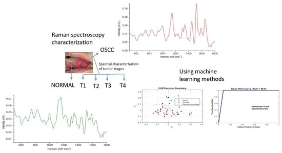
1. Introduction
2. Methods and Materials
2.1. Sample Collection and Preparation
2.2. Raman Spectroscopy Detection and Data Acquisition
2.3. Data Analysis
3. Results
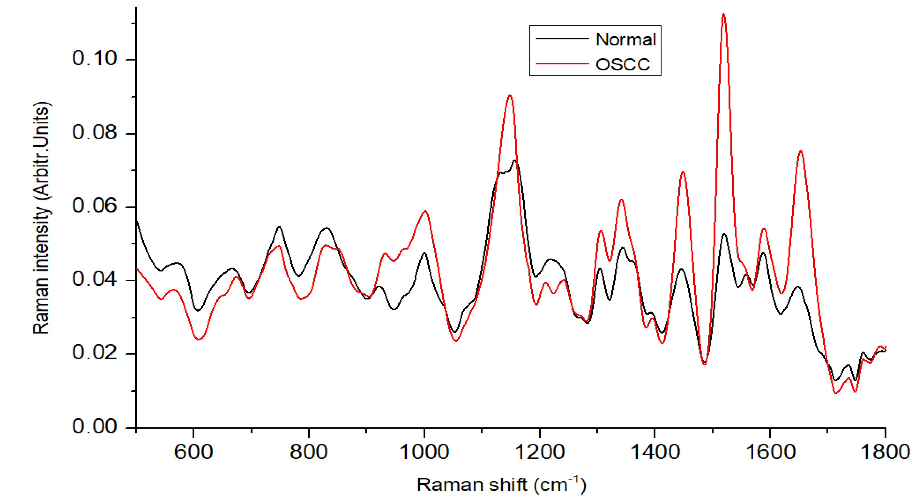
3.1. Spectral Features
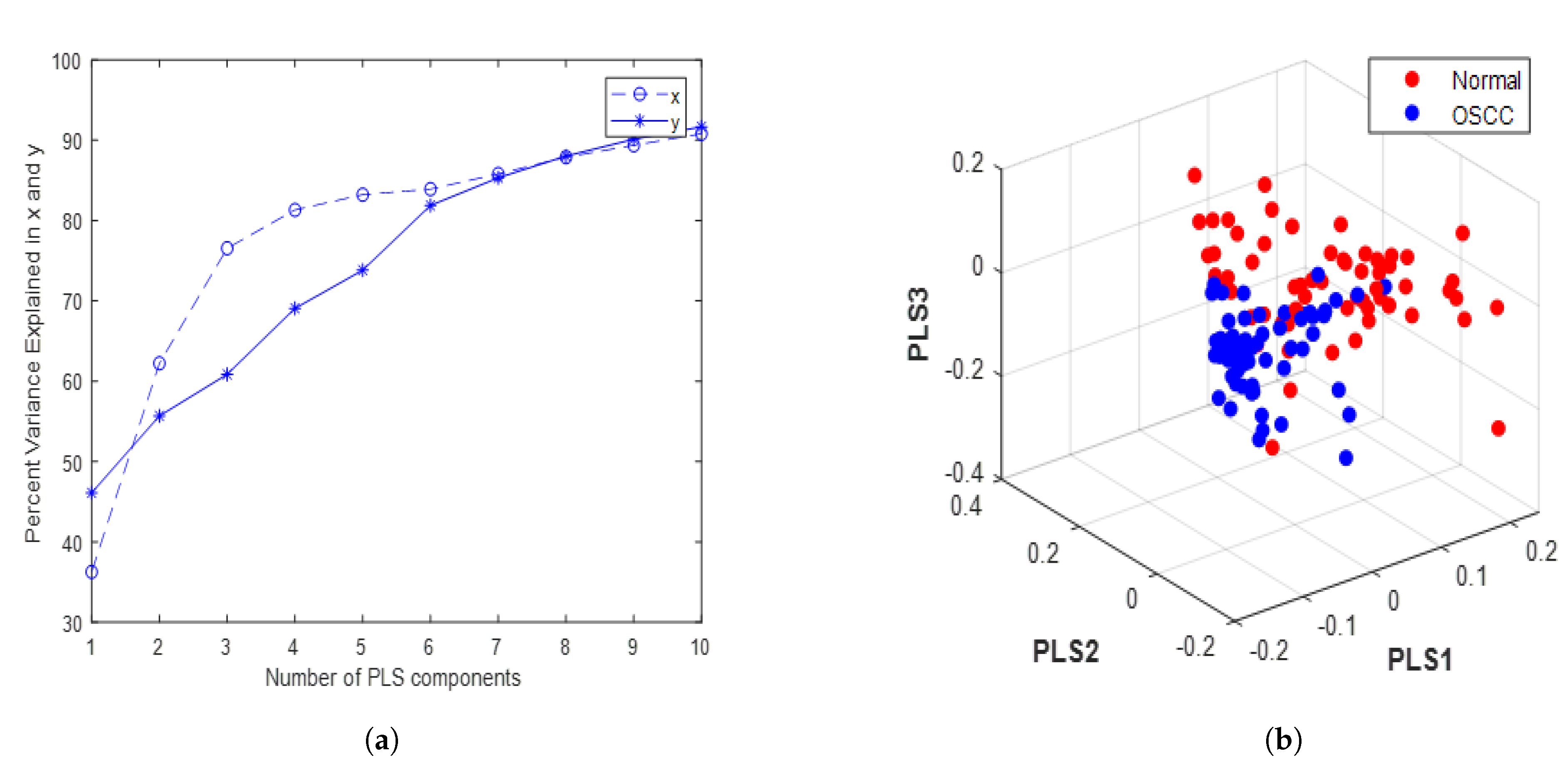
3.2. Optimization of PLS Components and Evaluation
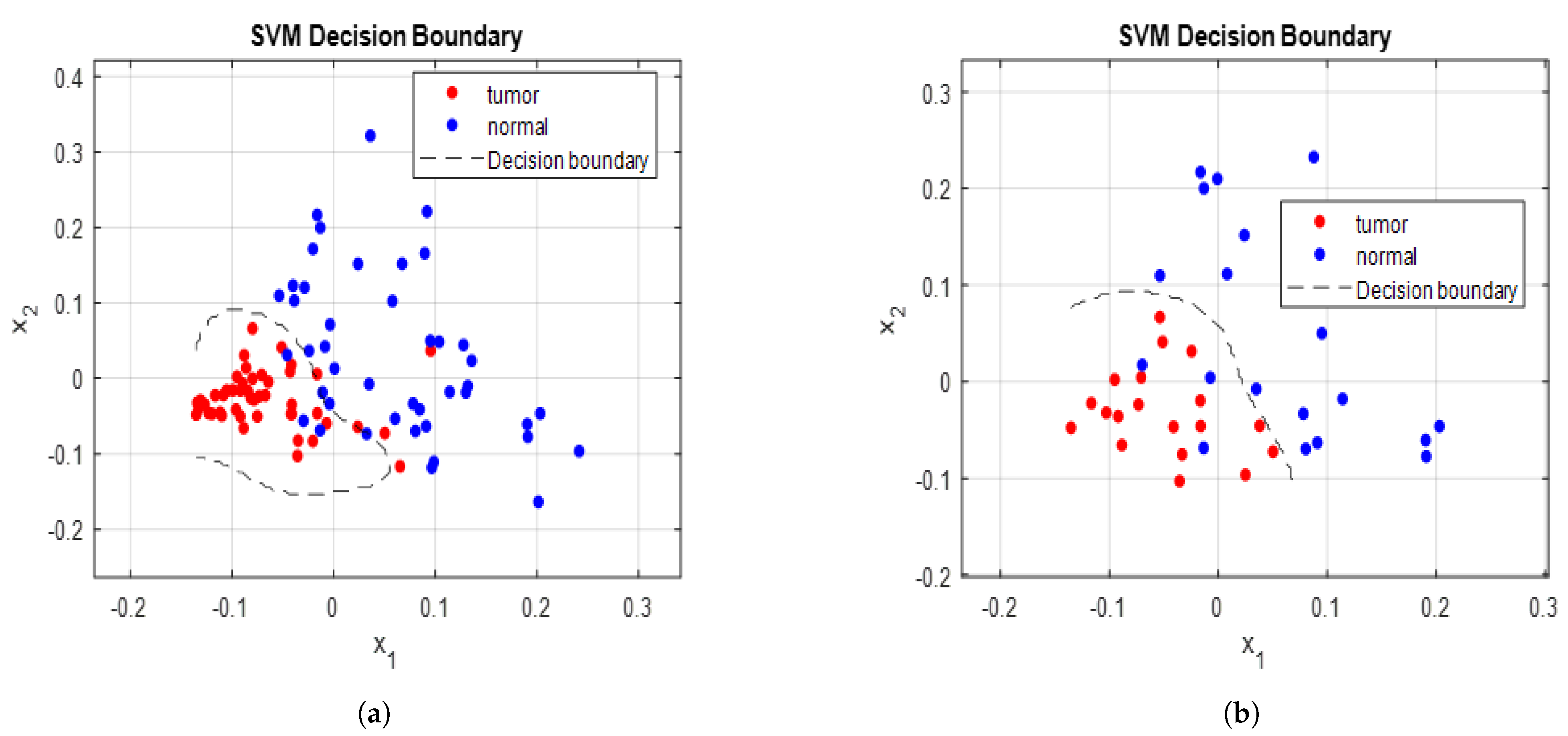
3.3. Training and Validation Procedure of SVM Model
3.4. Evaluation of Model Using Testing Set
4. Discussion
5. Conclusions
Author Contributions
Funding
Institutional Review Board Statement
Informed Consent Statement
Data Availability Statement
Conflicts of Interest
References
- Rai, P.; Goh, C.E.; Seah, F.; Islam, I.; Chia-Wei, W.W.; Mcloughlin, P.M.; Loh, J.S.P. Oral Cancer Awareness of Tertiary Education Students and General Public in Singapore. Int. Dent. J. 2023. [CrossRef]
- Chi, A.C.; Day, T.A.; Neville, B.W. Oral cavity and oropharyngeal squamous cell carcinoma—An update. CA Cancer J. Clin. 2015, 65, 401–421. [Google Scholar] [CrossRef]
- Sung, H.; Ferlay, J.; Siegel, R.L.; Laversanne, M.; Soerjomataram, I.; Jemal, A.; Bray, F. Global cancer statistics 2020: GLOBOCAN estimates of incidence and mortality worldwide for 36 cancers in 185 countries. CA Cancer J. Clin. 2021, 71, 209–249. [Google Scholar] [CrossRef] [PubMed]
- Jhuang, J.R.; Su, S.Y.; Chiang, C.J.; Yang, Y.W.; Lin, L.J.; Hsu, T.H.; Lee, W.C. Forecast of peak attainment and imminent decline after 2017 of oral cancer incidence in men in Taiwan. Sci. Rep. 2022, 12, 5726. [Google Scholar] [CrossRef]
- Bhatia, N.; Lalla, Y.; Vu, A.N.; Farah, C.S. Advances in optical adjunctive AIDS for visualisation and detection of oral malignant and potentially malignant lesions. Int. J. Dent. 2013, 2013, 194029. [Google Scholar] [CrossRef] [Green Version]
- Chakraborty, D.; Ghosh, D.; Kumar, S.; Jenkins, D.; Chandrasekaran, N.; Mukherjee, A. Nano-diagnostics as an emerging platform for oral cancer detection: Current and emerging trends. Wiley Interdiscip. Rev. Nanomed. Nanobiotechnol. 2023, 15, e1830. [Google Scholar] [CrossRef]
- Liu, D.; Zhao, X.; Zeng, X.; Dan, H.; Chen, Q. Non-invasive techniques for detection and diagnosis of oral potentially malignant disorders. Tohoku J. Exp. Med. 2016, 238, 165–177. [Google Scholar] [CrossRef] [Green Version]
- Jeng, M.J.; Sharma, M.; Chao, T.Y.; Li, Y.C.; Huang, S.F.; Chang, L.B.; Chow, L. Multiclass classification of autofluorescence images of oral cavity lesions based on quantitative analysis. PLoS ONE 2020, 15, e0228132. [Google Scholar] [CrossRef] [PubMed]
- Pence, I.; Mahadevan-Jansen, A. Clinical instrumentation and applications of Raman spectroscopy. Chem. Soc. Rev. 2016, 45, 1958–1979. [Google Scholar] [CrossRef] [PubMed] [Green Version]
- Cordero, E.; Latka, I.; Matthäus, C.; Schie, I.W.; Popp, J. In-vivo Raman spectroscopy: From basics to applications. J. Biomed. Opt. 2018, 23, 071210. [Google Scholar] [CrossRef]
- Saatkamp, C.J.; de Almeida, M.L.; Bispo, J.A.M.; Pinheiro, A.L.B.; Fernandes, A.B.; Silveira, L., Jr. Quantifying creatinine and urea in human urine through Raman spectroscopy aiming at diagnosis of kidney disease. J. Biomed. Opt. 2016, 21, 037001. [Google Scholar] [CrossRef] [PubMed] [Green Version]
- Jeng, M.J.; Sharma, M.; Sharma, L.; Chao, T.Y.; Huang, S.F.; Chang, L.B.; Wu, S.L.; Chow, L. Raman spectroscopy analysis for optical diagnosis of oral cancer detection. J. Clin. Med. 2019, 8, 1313. [Google Scholar] [CrossRef] [PubMed]
- Sharma, M.; Jeng, M.J.; Young, C.K.; Huang, S.F.; Chang, L.B. Developing an Algorithm for Discriminating Oral Cancerous and Normal Tissues Using Raman Spectroscopy. J. Pers. Med. 2021, 11, 1165. [Google Scholar] [CrossRef] [PubMed]
- Jeng, M.J.; Sharma, M.; Sharma, L.; Huang, S.F.; Chang, L.B.; Wu, S.L.; Chow, L. Novel Quantitative Analysis Using Optical Imaging (VELscope) and Spectroscopy (Raman) Techniques for Oral Cancer Detection. Cancers 2020, 12, 3364. [Google Scholar] [CrossRef] [PubMed]
- Fridman, E.; Na’ara, S.; Agarwal, J.; Amit, M.; Bachar, G.; Villaret, A.B.; Brandao, J.; Cernea, C.R.; Chaturvedi, P.; Clark, J.; et al. The role of adjuvant treatment in early-stage oral cavity squamous cell carcinoma: An international collaborative study. Cancer 2018, 124, 2948–2955. [Google Scholar] [CrossRef]
- Wang, R.; Wang, Y. Fourier transform infrared spectroscopy in oral cancer diagnosis. Int. J. Mol. Sci. 2021, 22, 1206. [Google Scholar] [CrossRef]
- Chen, P.H.; Shimada, R.; Yabumoto, S.; Okajima, H.; Ando, M.; Chang, C.T.; Lee, L.T.; Wong, Y.K.; Chiou, A.; Hamaguchi, H.o. Automatic and objective oral cancer diagnosis by Raman spectroscopic detection of keratin with multivariate curve resolution analysis. Sci. Rep. 2016, 6, 20097. [Google Scholar] [CrossRef] [Green Version]
- Dai, W.Y.; Lee, S.; Hsu, Y.C. Discrimination between oral cancer and healthy cells based on the adenine signature detected by using Raman spectroscopy. J. Raman Spectrosc. 2018, 49, 336–342. [Google Scholar] [CrossRef]
- Knipfer, C.; Motz, J.; Adler, W.; Brunner, K.; Gebrekidan, M.T.; Hankel, R.; Agaimy, A.; Will, S.; Braeuer, A.; Neukam, F.W.; et al. Raman difference spectroscopy: A non-invasive method for identification of oral squamous cell carcinoma. Biomed. Opt. Express 2014, 5, 3252–3265. [Google Scholar] [CrossRef] [Green Version]
- Kerr, L.T.; Byrne, H.J.; Hennelly, B.M. Optimal choice of sample substrate and laser wavelength for Raman spectroscopic analysis of biological specimen. Anal. Methods 2015, 7, 5041–5052. [Google Scholar] [CrossRef] [Green Version]
- Jeng, M.J.; Sharma, M.; Lee, C.C.; Lu, Y.S.; Tsai, C.L.; Chang, C.H.; Chen, S.W.; Lin, R.M.; Chang, L.B. Raman Spectral Characterization of Urine for Rapid Diagnosis of Acute Kidney Injury. J. Clin. Med. 2022, 11, 4829. [Google Scholar] [CrossRef] [PubMed]
- Liu, W.; Sun, Z.; Chen, J.; Jing, C. Raman spectroscopy in colorectal cancer diagnostics: Comparison of PCA-LDA and PLS-DA models. J. Spectrosc. 2016, 2016, 1603609. [Google Scholar] [CrossRef] [Green Version]
- Liu, D.; Guo, W. Identification of kiwifruits treated with exogenous plant growth regulator using near-infrared hyperspectral reflectance imaging. Food Anal. Methods 2015, 8, 164–172. [Google Scholar] [CrossRef]
- Guze, K.; Pawluk, H.C.; Short, M.; Zeng, H.; Lorch, J.; Norris, C.; Sonis, S. Pilot study: Raman spectroscopy in differentiating premalignant and malignant oral lesions from normal mucosa and benign lesions in humans. Head Neck 2015, 37, 511–517. [Google Scholar] [CrossRef] [PubMed]
- Rau, J.V.; Fosca, M.; Graziani, V.; Taffon, C.; Rocchia, M.; Caricato, M.; Pozzilli, P.; Onetti Muda, A.; Crescenzi, A. Proof-of-concept Raman spectroscopy study aimed to differentiate thyroid follicular patterned lesions. Sci. Rep. 2017, 7, 14970. [Google Scholar] [CrossRef] [Green Version]
- Malini, R.; Venkatakrishna, K.; Kurien, J.; Pai, K.M.; Rao, L.; Kartha, V.; Krishna, C.M. Discrimination of normal, inflammatory, premalignant, and malignant oral tissue: A Raman spectroscopy study. Biopolym. Orig. Res. Biomol. 2006, 81, 179–193. [Google Scholar] [CrossRef]
- Movasaghi, Z.; Rehman, S.; Rehman, I.U. Raman spectroscopy of biological tissues. Appl. Spectrosc. Rev. 2007, 42, 493–541. [Google Scholar] [CrossRef]
- Huang, Z.; McWilliams, A.; Lui, H.; McLean, D.I.; Lam, S.; Zeng, H. Near-infrared Raman spectroscopy for optical diagnosis of lung cancer. Int. J. Cancer 2003, 107, 1047–1052. [Google Scholar] [CrossRef]
- Abdi, H. Partial least squares regression and projection on latent structure regression (PLS Regression). Wiley Interdiscip. Rev. Comput. Stat. 2010, 2, 97–106. [Google Scholar] [CrossRef]
- Kohavi, R. A study of cross-validation and bootstrap for accuracy estimation and model selection. In Proceedings of the IJCAI’95: Proceedings of the 14th International Joint Conference on Artificial Intelligence, Montreal, QC, Canada, 20–25 August 1995; Volume 14, pp. 1137–1145.
- Geladi, P.; Kowalski, B.R. Partial least-squares regression: A tutorial. Anal. Chim. Acta 1986, 185, 1–17. [Google Scholar] [CrossRef]
- Gareth, J.; Daniela, W.; Trevor, H.; Robert, T. An Introduction to Statistical Learning: With Applications in R; Spinger: Berlin/Heidelberg, Germany, 2013. [Google Scholar]
- Wang, K.; Qiu, Y.; Wu, C.; Wen, Z.N.; Li, Y. Surface-enhanced Raman spectroscopy and multivariate analysis for the diagnosis of oral squamous cell carcinoma. J. Raman Spectrosc. 2023, 54, 355–362. [Google Scholar] [CrossRef]
- Carvalho, L.F.C.; Nogueira, M.S.; Bhattacharjee, T.; Neto, L.P.; Daun, L.; Mendes, T.O.; Rajasekaran, R.; Chagas, M.; Martin, A.A.; Soares, L.E.S. In vivo Raman spectroscopic characteristics of different sites of the oral mucosa in healthy volunteers. Clin. Oral Investig. 2019, 23, 3021–3031. [Google Scholar] [CrossRef] [PubMed]


| Characteristics | Age (Mean ± SD) | Gender (M:F) | |||
|---|---|---|---|---|---|
| 55.4 ± 12.8 | 59:5 | ||||
| Location | Tongue | 14 (21.9%) | |||
| Mouth floor | 5 (7.8%) | ||||
| Lip | 2 (3%) | ||||
| Buccal mucosa | 28 (43.8%) | ||||
| Alveolus (gum) | 14 (21.9%) | ||||
| Retromolar trigone | 1 (1.6%) | ||||
| Tumor Stage | T1 | T2 | T3 | T4 | |
| 6 (9.5%) | 17 (26.3%) | 10 (15.7%) | 31 (48.5%) | ||
| Number of PLS Components | Computation Time (in msec) with Classifier |
|---|---|
| 2 | 7.1 |
| 5 | 7.6 |
| 10 | 9.9 |
| PLS-SVM | SEN | SPE | AC | PRE | BAC | F1-Score | MCC |
|---|---|---|---|---|---|---|---|
| Parameters | 95.65 | 93.33% | 94.74% | 95.65% | 94.49% | 95.65% | 0.889 |
Disclaimer/Publisher’s Note: The statements, opinions and data contained in all publications are solely those of the individual author(s) and contributor(s) and not of MDPI and/or the editor(s). MDPI and/or the editor(s) disclaim responsibility for any injury to people or property resulting from any ideas, methods, instructions or products referred to in the content. |
© 2023 by the authors. Licensee MDPI, Basel, Switzerland. This article is an open access article distributed under the terms and conditions of the Creative Commons Attribution (CC BY) license (https://creativecommons.org/licenses/by/4.0/).
Share and Cite
Sharma, M.; Li, Y.-C.; Manjunatha, S.N.; Tsai, C.-L.; Lin, R.-M.; Huang, S.-F.; Chang, L.-B. Identification of Healthy Tissue from Malignant Tissue in Surgical Margin Using Raman Spectroscopy in Oral Cancer Surgeries. Biomedicines 2023, 11, 1984. https://doi.org/10.3390/biomedicines11071984
Sharma M, Li Y-C, Manjunatha SN, Tsai C-L, Lin R-M, Huang S-F, Chang L-B. Identification of Healthy Tissue from Malignant Tissue in Surgical Margin Using Raman Spectroscopy in Oral Cancer Surgeries. Biomedicines. 2023; 11(7):1984. https://doi.org/10.3390/biomedicines11071984
Chicago/Turabian StyleSharma, Mukta, Ying-Chang Li, S. N. Manjunatha, Chia-Lung Tsai, Ray-Ming Lin, Shiang-Fu Huang, and Liann-Be Chang. 2023. "Identification of Healthy Tissue from Malignant Tissue in Surgical Margin Using Raman Spectroscopy in Oral Cancer Surgeries" Biomedicines 11, no. 7: 1984. https://doi.org/10.3390/biomedicines11071984